Article

Hydrological Functioning and Water Availability in a Himalayan Karst Basin under Climate Change

1
Department of Earth and Environmental Sciences, University of Kentucky, Lexington, KY 40506, USA
2
Kentucky Geological Survey, University of Kentucky, Lexington, KY 40506, USA
3
Department of Earth Sciences, University of Kashmir, Srinagar 190006, India
*
Author to whom correspondence should be addressed.
Sustainability 2023, 15(11), 8666; https://doi.org/10.3390/su15118666
Submission received: 18 April 2023 / Revised: 20 May 2023 / Accepted: 21 May 2023 / Published: 26 May 2023
(This article belongs to the Section Sustainable Water Management)

Abstract

:
Karst springs are important water sources for both human needs and environmental flows. The responses of karst springs to hydrometeorological factors vary depending on local conditions. In this study, we investigated Martandnag spring in the Liddar catchment in the Kashmir valley of northern India. We used statistical time series (autocorrelation and cross-correlation) and machine-learning (ML) techniques (random forest regression (RFR) and support vector regression (SVR)) to characterize how rainfall, temperature, and snow cover affect the karst spring flow and predict the future responses of the spring stage based on climate scenarios, in the Intergovernmental Panel on Climate Change Assessment Report 6. The statistical time series showed that the memory effect of Martandnag spring varies from 43 to 61 days, indicating moderate karstification and a relatively high storage capacity of the karst aquifer in the Liddar catchment. The delay between recharge and discharge varies from 13 to 44 days, and it is more strongly correlated to snow/ice melt than to rainfall. The ML analysis shows that SVR outperformed RFR in predicting spring flow. Under all climate scenarios, a trained SVR model showed that spring flow increased during the late winter to early spring, and decreased during the summer (except in August) and in autumn. Scenarios with increased greenhouse gas emissions further reduced flow in the summer and autumn. These predictions can be helpful for water-resource planning in similar watersheds in the Western Himalayas.

1. Introduction

Karst landscapes are characterized by sinkholes, sinking streams, conduits, caves, and springs, which integrate surface and subsurface drainage. Karst regions occupy 15% of Earth’s ice-free land surface [1], and almost a quarter of the world’s population directly or indirectly depend on karst water supplies [2]. Groundwater flow in karst aquifers is characterized by a complex interplay of fast-flowing conduits and slow-flowing matrix systems [3,4]. Karst groundwater systems are vulnerable to environmental changes and can be potent indicators of climate change and anthropogenic effects on hydrological processes [5,6].
The responses of karst aquifers to hydrometeorological factors (e.g., precipitation and temperature) vary depending on local conditions. Climate-based hydrological changes can increase stresses on groundwater resources to meet the increasing demand for drinking water, irrigation, and industrial purposes [7]. The global average surface temperature over 2001–2020 was 0.99 °C higher than over 1800–1900 [8]. The Intergovernmental Panel on Climate Change (IPCC) regional temperature trends show a similar increasing pattern for the future [8]. Projected mean temperature rises range from 1.0 to 1.4 °C for 2046–2065, and from 1.0 to 3.7 °C for 2081–2100 [8]. In the Indian subcontinent, the mean temperature is projected to rise 2.1–2.6 °C by 2050 and 3.1–3.6 °C by 2080 [9]. These changes are predicted to impact freshwater availability, biodiversity, agriculture, and human health [9].
Carbonate rocks are widely distributed in the Kashmir valley of the Western Himalayas in northern India, with the greatest karstification occurring in the southern parts of the valley. Karst springs in this region provide freshwater to more than one million people for drinking and agriculture [10]. Meltwater generated from snow and glaciers is a crucial contributor to the hydrological budget in this region [11,12]. The spring discharge decreases during low-flow periods, which increases the pressure on karst water resources [11]. The transition from snow to rainfall due to the changing climate may severely affect the region’s water resources in the future, especially in summer, due to the high demand for agriculture [12].
Multiple studies on the hydrology of the Kashmir valley have been conducted in recent years. Jeelani et al. (2012) examined the relative contributions of snowmelt and ice melt to the overall runoff, and changes in runoff timing and quantity to the Liddar watershed over the period of 1901–2010 for comparison with future climate conditions [13]. They found that snowmelt contributes ~60% of the total annual flow in the Liddar River, while only 2% is from glacial melt [13]. Environmental tracers (e.g., Cl, δ18O, and δ2H) have been used to characterize hydrological processes and to quantify the contribution of different source waters (springs and streams) [11,12,14,15,16]. The tracer studies suggest that because of significant snow cover and glaciers, the heavier isotope signals of rainfall in summer have a negligible impact on the isotopic composition of streams and karst springs [12]. Shah et al. (2018) conducted thorough fieldwork to develop a karst inventory and speleological database for the Kashmir Himalaya [17]. However, no studies in the Kashmir valley have used time-series analyses to examine the responses of springs to meteorological forcings or have used machine-learning (ML) techniques to predict future water availability.
In recent years, multiple studies have used artificial neural networks (ANNs) or their subgroup of deep learning in modeling karst water resources. ANNs were found to predict karst spring flow accurately where field data were abundant (e.g., [18]). Paleologos et al. (2013) used an ANN (e.g., multi-layer perceptron back-propagation neural network) to predict the flows of two karst springs in Crete (Greece), based on limited field data [19]. The predictions captured the characteristics of both springs, and under-/over-estimations of observed discharges were within 3% [19]. Convolutional neural networks have been found to be more useful than long short-term memory for modeling karst spring discharge [20,21]. Goyal et al. (2017) used support vector regression (SVR) [22] to predict the discharge of the same springs studied by [19]. SVR outperformed generalized regression neural networks and radial basis function (RBF) neural networks, given the scarcity and irregular data collection of the spring flow rate [22].
Our study focuses on Martandnag spring, located in the Liddar watershed in the southeastern part of the Kashmir valley. We used statistical time series (autocorrelation and cross-correlation), and supervised ML algorithms (random forest regression (RFR) and SVR) to characterize the karst aquifer and to predict future spring stage using climate scenarios in [8]. Numerous studies have used time-series analysis to describe the behaviors of karst aquifers worldwide [23,24,25,26]. However, time-series analysis is limited to characterizing the hydrologic functioning and behavior of a karst system, and cannot forecast future water scenarios. Thus, we explored the compatibilities of different ML approaches to simulate spring stage and to predict future water availability in the Liddar watershed.

2. Materials and Methods

2.1. Study Area

The Liddar catchment is located in Anantnag district, Jammu and Kashmir, India (Figure 1). The catchment lies within the basin of the upper Jhelum River, a tributary of the Indus River. The catchment area is ~1245 km2, constituting ~10% of the total Jhelum River basin [27]. The altitude of the catchment ranges from ~1550 to 5400 m above sea level (Figure 1). Two moisture-laden wind systems dominate the region: the mid-latitude circulation (also known as the western disturbances), originating from the Atlantic Ocean, Mediterranean Sea, and Black Sea, and the Indian summer monsoon from the Indian Ocean, the Bay of Bengal, and the Arabian Sea [16,28].
Slightly more than half (58%) of the Kashmir valley is covered by karstified carbonate rocks, with Triassic limestone comprising the primary aquifer [17]. The geology of the Liddar catchment is characterized by diverse lithologies ranging from Paleozoic sedimentary to recent alluvium [29,30,31], but is dominated by a >1000 m thick sequence of Triassic limestone and dolomite, with some interbedded sandstone and shale [14]. Lacustrine sandstones, loess, and conglomerates of the Pleistocene Karewa Group overlie the limestone [14,28]. Small, dissected valleys between Triassic limestone ridges and the Karewa Group are filled with recent alluvium comprising fine silt and mud, but boulders and coarse sediment are common along streams. Groundwater discharges through springs at the contact between Triassic limestone and low-permeability alluvium [14]. Martandnag spring is one of the main cold springs (temperature: 8–14 °C) in the catchment [28]. The discharge of the cold springs is highly variable, ranging from 50 to 5000 L/s seasonally [28]. The highly fluctuating discharge, and the quick response of the spring flow to rainfall and snowmelt are indicative of a well-developed karstic drainage system in this region [10].
Land cover in the Liddar catchment is predominantly rangeland (39%) and forest (26%), followed by permanent snow and ice cover (15%), cropland (e.g., corn, wheat, and soybean; 9%), minor developed area (5%), bare ground (5%), and waterbodies (1%) [32]. From 2017 to 2021, the permanent snow and ice cover increased from 3% to 15%, and the built-up area increased by 2% in 2021 [32]. Cropland and built-up areas are prevalent in downstream parts of the catchment.

2.2. Data Acquisition

Hourly stage data were collected using an OTT Orpheus Mini/OTT-CTD datalogger (Hydromet, Germany) at Martandnag spring from April 2013 to June 2016, and May 2019 to August 2020. Daily rainfall, and maximum and minimum temperature records from 2013 to 2020 were procured from the Indian Meteorological Department (IMD) for the Pahalgam weather station, 32 km north of Martandnag. Monthly snow-cover data from April 2013 to December 2020 were derived from the Landsat 8 Operational Land Imager/Thermal Infrared Sensor (OLI/TIRS) collection 2 Level-2 Science Products (L2SP) [33]. The L2SP dataset contains atmospherically corrected surface reflectance and land-surface temperature. Landsat 8 OLI/TIRS has a spatial resolution of 30 m and comprises 11 bands, including five visible and near-infrared, and two shortwave infrared bands. The temporal resolution of Landsat 8 is 16 days, but some months have only one record due to the overlapped area of images. The cloud coverage was typically less than 15% for all of the images used for this analysis, but images for November 2020 were excluded due to high cloud contamination. Detailed data descriptions, including Landsat 8 OLI/TIRS, are given in Table 1.

2.3. Data Analysis

All hydrometeorological data were analyzed for summary statistics. Pearson’s product moment correlation was applied to examine the correlation between parameters. The Mann-Kendall trend test was also implemented to examine any significant trend for all parameters. All analyses were conducted in R version 4.2.2 and Rstudio version 2022.12.0 [34].

2.3.1. Snow Cover

Remote sensing techniques are widely used for the determination of snow-covered area (SCA) [35,36]. Snow is highly reflective in the visible green wavelength, and is highly absorbable in the shortwave infrared part of the electromagnetic spectrum [36]. The monthly SCA of the Liddar watershed was derived using the normalized difference snow index (NDSI), which compares the difference in the reflectance in the visible (band 3; wavelength 0.53–0.59 µm) and shortwave infrared (band 6; wavelength 1.57–1.66 µm) parts of the spectrum [37]. The Landsat 8 OLI/TIRS products collect the snow-cover data in NDSI format using the following equation [37]:
NDSI = ((band 3 − band 6)/(band 3 + band 6))
The NDSI value ranges from +1 to −1; pixels without snow tend to have lower values. The NDSI threshold for snow coverage is commonly considered to be > 0.4 [37,38,39,40]. However, the NDSI threshold varies seasonally and changes between forested and open areas [40,41]. In our analysis, pixels with NDSI > 0.5 are considered as snow-covered [42]. We calculated the SCA and the area percentage for the Liddar watershed from April 2013 to December 2020. The monthly snow cover was converted to daily records via linear interpolation. The NDSI analysis was performed in ArcGIS 10.8.

2.3.2. Statistical Time-Series Analysis

The autocorrelation function (ACF) quantifies the system’s memory effect by calculating successive values’ linear dependencies over time [43]. The auto-correlogram indicates the system’s memory, which is computed by the decorrelation of lag time [44]. The threshold of the autocorrelation function (rk) varies from 0.1 to 0.2, beyond which white noise dominates the system [23]. The structure and shape of the correlogram indicate the storage capacity and degree of karstification [44,45]. We calculated the ACF separately on hourly and average daily stage values over 2013–2016 and 2019–2020.
The cross-correlation function (CCF) examines the relationship between input signals, such as precipitation or concentrated infiltration, and the output signals, such as spring discharge or stage, thus indicating the impulse response of a karst system [23,45,46]. The mean response time of an aquifer to a rainfall event can be computed from this analysis. The delay between precipitation, and spring stage or discharge (from lag 0 to a maximum CCF value) shows the pressure-pulse transfer time through the aquifer [47]. Cross-correlation analysis requires consistently paired time series, so we used daily data for the CCF calculation for spring stage, rainfall, and the maximum and minimum air temperatures. Because the stage data from June 2016 to April 2019 were missing, we conducted a cross-correlation analysis between stage and rainfall, stage and maximum air temperature, and stage and minimum air temperature on the available data for the periods 2013–2016 and 2019–2020 for Martandnag spring.

2.3.3. Machine-Learning Models

Random Forest Regression

Random forest is an ensemble learning method that combines multiple decision trees and predicts the final output based on the average of each tree prediction. RFR uses bagging or bootstrap aggregation techniques in which the aggregated decision tree runs in parallel without interacting. RFR algorithms take advantage of the randomness of sample and feature selection to prevent overfitting and to limit noise [48,49]. However, RFR cannot extrapolate the linear trend to predict new examples with a value beyond those seen in the training data. More details about the model and algorithms are available in [50].
Our analysis used RFR based on five variables to predict the spring stage. We built three RF models using different predictor variables. Model I predicted the spring stage as a function of the monthly mean rainfall, minimum air temperature, maximum air temperature, average air temperature, and SCA. Model II explored the impact of rainfall on recharge by excluding SCA from model I. Mean daily data were used for all variables in model II. Model III added the daily snow-cover data calculated via linear interpolation to model II. For each model, we split the entire dataset into training and test sets to construct the models. Eighty percent of the data was used for training, and the remaining 20% was used for model testing. The best model was selected by comparing the root mean square error (RMSE) and the coefficient of determination (R2).

Support Vector Regression

The support vector machine (SVM) approach for classification, and regression was developed by [51]. For a simple linear regression problem trained on the dataset (X, Y), where X = {x1, x2, …,xn} is the input dataset and Y = {y1, y2, …, yn} is the target dataset, the goal of SVR is to identify a function f(x) with a maximum deviation ɛ from the target variable for all the training data. In addition, the function f(x) should be as flat as possible [52,53]. The advantage of SVR is its ability to map the input vector in a higher dimensional space (i.e., a hyperplane) and to keep the regression in linear form without changing the predictor variables. The SVR technique performs such operations through the kernel function.
We tested three SVR models using the same predictor variables as for RFR, with 80% of the data being used for model training, and the remaining 20% being used for testing the model. We used four SVR kernel functions (linear, polynomial, radial basis, and sigmoid) to account for the nonlinearity in the data sets, and compared them to find the best model based on RMSE and R2 values.

Hyperparameter Selection

From a conceptual perspective, setting the optimum hyperparameters is critical to obtain the best predictions for data-driven models such as RFR and SVR. Unlike ANNs, RFR needs two parameters to generate a prediction model: the number of regression trees and the number of variables used in each node to grow the regression tree [54]. To optimize these two parameters, we experimented with different numbers of regression trees and split the evidential features to obtain acceptable model outputs. We set the value of the number of trees from 1 to 1000, and the variables in each split from 1 to 5.
The performance of SVR depends on the optimizations of its hyperparameters, such as the SVR constant ε, the cost function C, and gamma (RBF and sigmoid kernels parameter) [22,53]. Initially, a gridded search method was used to find the optimum values of the SVR parameters. However, because of our relatively small dataset, each kernel’s default hyperparameter values were used to train the model.

2.3.4. Prediction of Spring Stage in 2030

We used projected climate change data for the near-term period (2021–2040) relative to 1995–2014 for four scenarios [8] to predict the Martandnag spring stage in 2030. The IPCC Assessment Report (AR) 6 used the simulation results from the Coupled Model Intercomparison Project 6 (CIMP6) to develop a new set of emission scenarios known as shared socio-economic pathways (SSPs), based on different socio-economic assumptions [55]. In IPCC AR 5, four representative concentration pathways (RCPs) were used, based on future greenhouse gas emissions and global effective radiative forcing. The RCP scenarios combined with SSPs have been incorporated into CIMP6, giving the updated scenarios SSP1-2.6, SSP2-4.5, SSP4-6.0, and SSP5-8.5, plus a new scenario (SSP3-7.0) [8]. We did not use scenario SSP4-6.0 in our predictions.
We obtained meteorological data for 2030 from the IPCC AR 6 Working Group I (WGI) Interactive Atlas [56] for the Tibetan Plateau (TIB) climate zone. Most Hindu Kush-Himalayan areas, including the Liddar watershed, lie in this zone. To predict the spring stage, we extracted the monthly data for mean air temperature, maximum air temperature, minimum air temperature, total rainfall, and snowfall for 2030. We used the IPCC CIMP6 projected snowfall data as a proxy for SCA for 2030. From [56], we extracted the monthly average of snowfall records for current climate conditions from 2013 to 2020. We then calculated the percentage of changes in monthly average snowfall for 2030, acquired from the IPCC CIMP6 model. We applied a similar percentage of changes to estimate the SCA for future prediction. We also used the WGI Interactive Atlas seasonal stripes column to extract the monthly climate change data for our analysis. The detailed IPCC projected climate change records for TIB used here are included in supplemental Table S1. The best-performing ML model was used to predict the monthly spring stage for 2030 at Martandnag.

3. Results

3.1. Summary Statistics

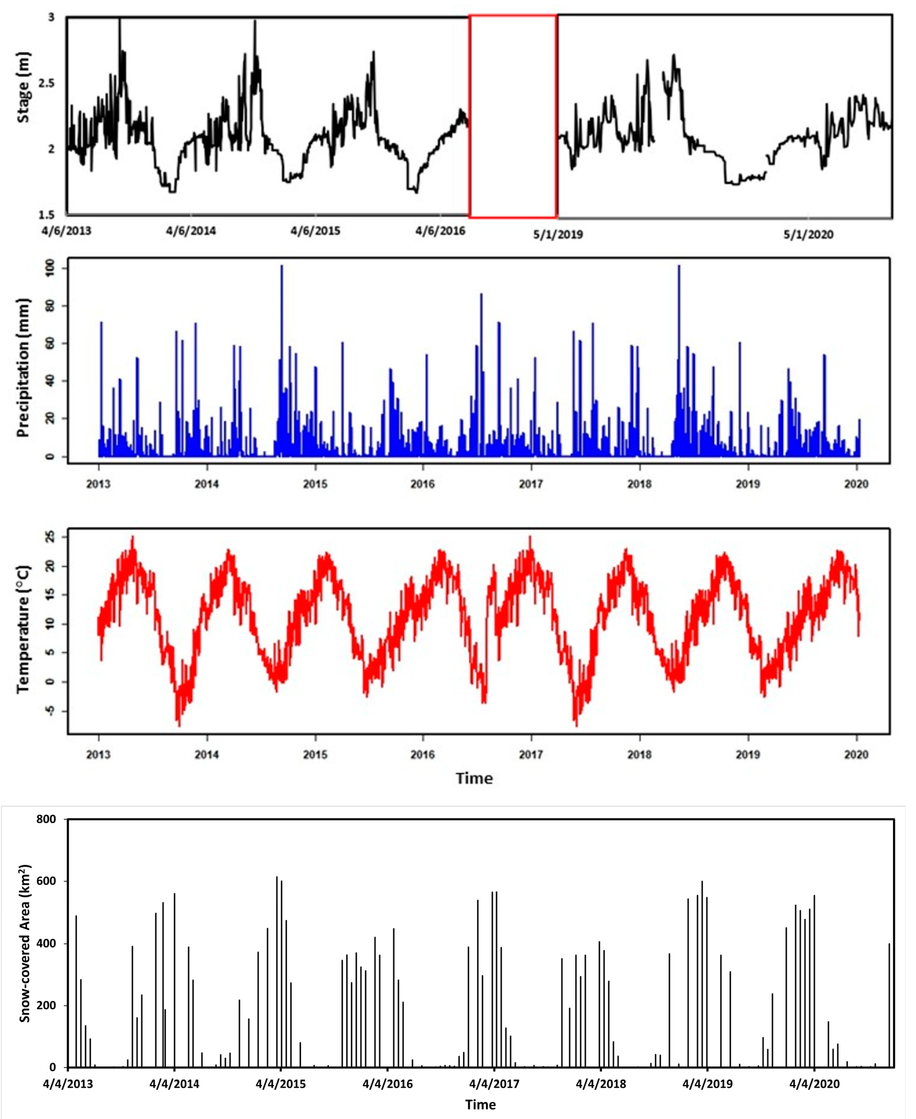
The mean stage of Martandnag spring was 2.07 m relative to the local datum; the stage was lowest in January (minimum 1.67 m) and highest in September (maximum 3.0 m) throughout the study period (Figure 2). The spring stage is significantly negatively correlated (r = −0.70) with SCA and significantly positively correlated (r = 0.71) with the maximum air temperature. We observed a significant downward trend in the spring stage (τ = −0.06, p = 0.001), and in the maximum (τ = −0.12, p < 0.001) and minimum air temperatures (τ = −0.12, p < 0.001) for the study period, but no significant trend in rainfall was identified (Figure 2).
The maximum 1-day total rainfall was recorded on 26 January 2017 (115 mm). Over 2013–2019, the mean annual rainfall in the Liddar catchment was 1253 mm (range 860–1557 mm). The total 1-day rainfall tended to be highest over late winter to spring, whereas the daily rainfall during the summer monsoon was limited (2–5 mm).
From 2013–2019, the annual average air temperature was 10 °C, ranging from −15 °C in January to 30 °C in July. The air temperature is negatively correlated (r = −0.72) to the basin’s SCA. The average daily air temperature was below freezing (<0 °C) for ~ 95 days each year. The snow-covered area was lowest from July to September (0–3%), and highest from January to April (30–60%). Summary statistics of stage, rainfall, air temperatures, and snow-covered area are given in Table 2.

3.2. Autocorrelation and Cross-Correlation

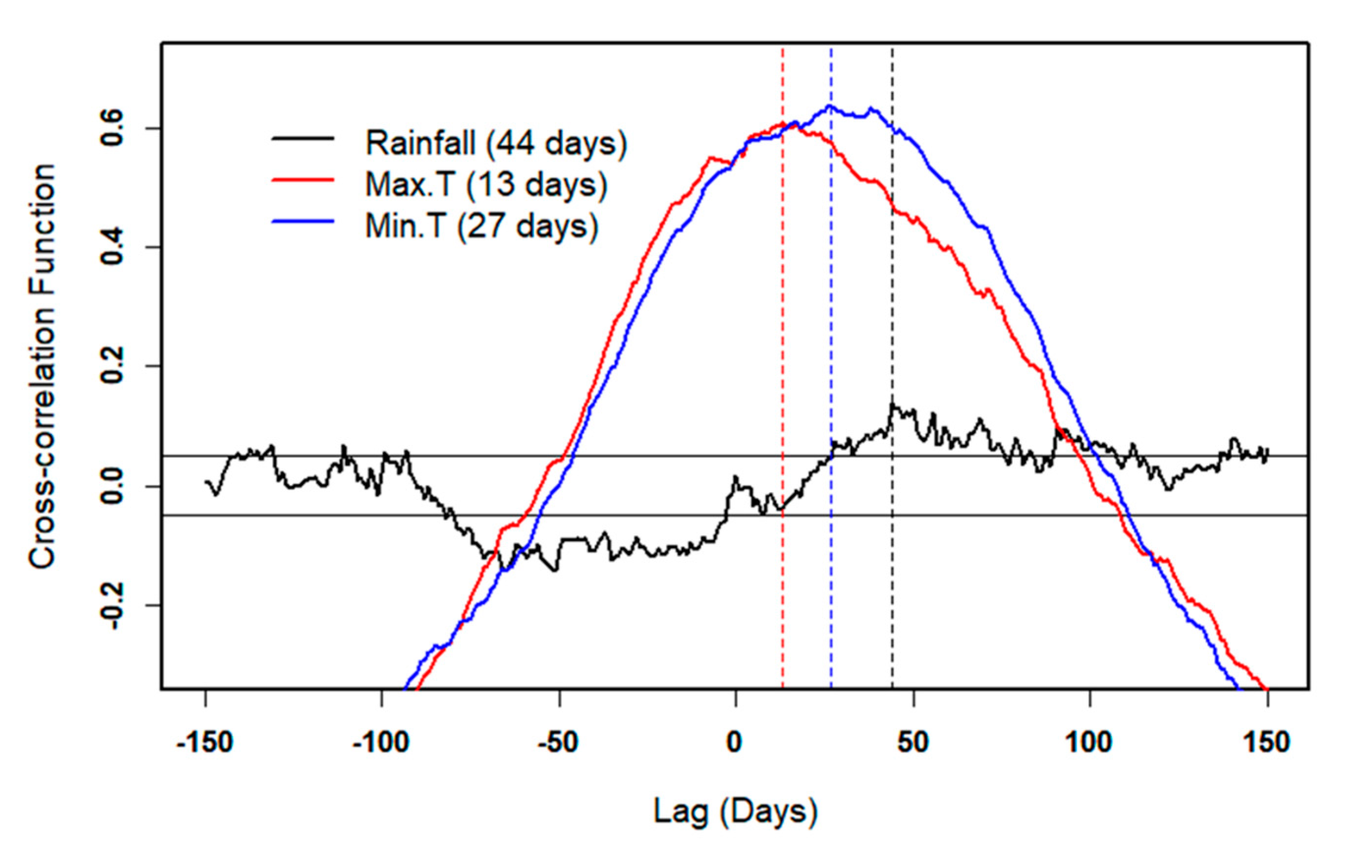
The autocorrelation functions for the hourly and daily stage values show that Martandnag spring has a high storage capacity. The memory effect (based on rk = 0.2) was somewhat longer for 2013–2016 (59 days for the daily stage and 61 days for the hourly stage; Figure 3) than for 2019–2020 (43 days for the hourly stage and 53 days for the daily stage). The cross-correlograms between daily rainfall and spring stage, and between daily air temperature and spring stage for 2013–2020 are shown in Figure 4. The CCF lag time (Tlag) between rainfall and spring stage is 44 days at a CCF value (Cxy(k)) of 0.14. The peak CCF values for air temperature and spring stage are higher (Cxy(k) = 0.60 for the maximum temperature and Cxy(k) = 0.63 for the minimum temperature), and they correspond to shorter Tlag values (13 and 27 days, respectively).

3.3. Machine-Learning Model Results

The best results were obtained using model I, and the worst results were obtained using model II, for both RFR and SVR (Table 3). This indicates that the monthly average records for all predictor variables can better predict the spring stage than the daily records for both RFR and SVR. The RFR models suggested that the variables that most influenced the spring stage were SCA, and maximum and minimum air temperatures, whereas rainfall was the least important parameter. The RMSE and R2 values for RFR model I are 0.10 and 0.74, respectively. For the SVR model, the RBF kernel shows the best agreement with the observed stage (RMSE = 0.06, R2 = 0.81). Therefore, we selected SVR model I to simulate the spring stage in 2030.

3.4. Model Prediction for IPCC Climate Change Scenarios

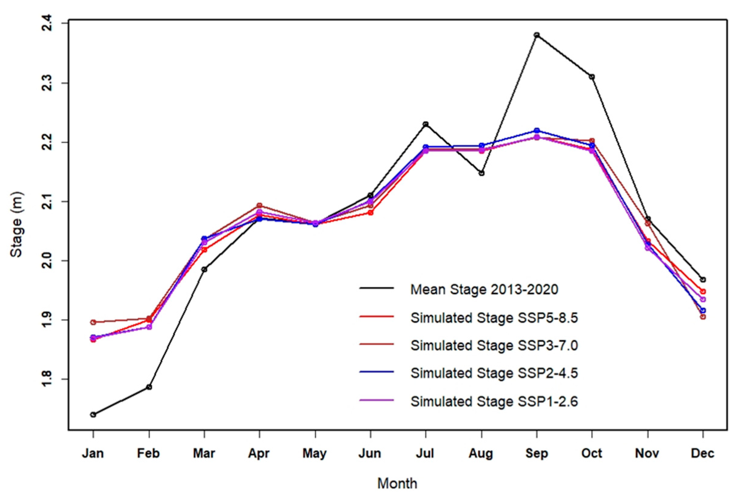
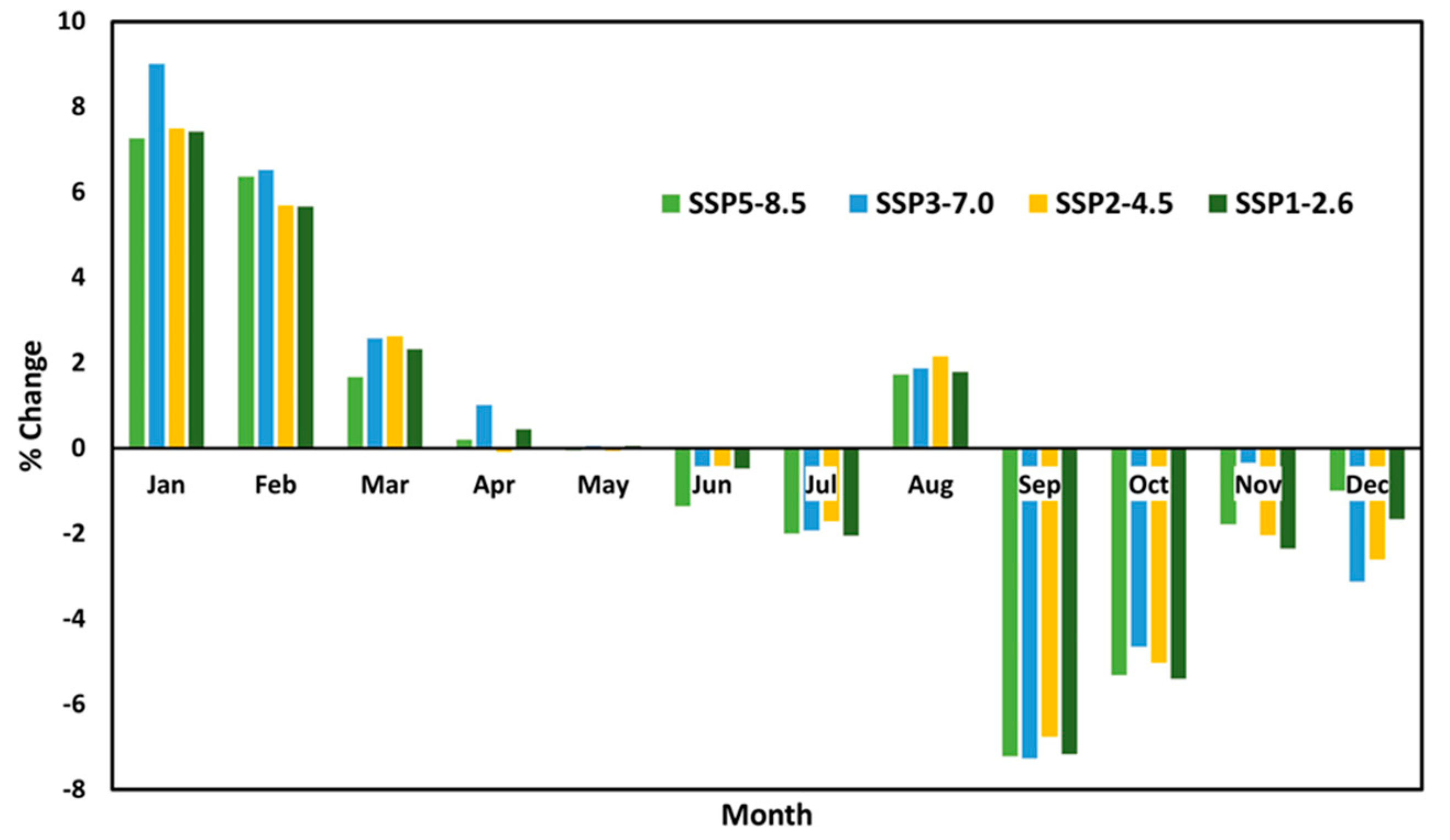
Under all scenarios, the stage of Martandnag spring increases during late winter to early spring, and decreases during summer (except in August) and autumn (Figure 5). The projected spring stage is ~5–7% lower over September–October 2030 relative to the current state (Figure 6). All scenarios show increases in the spring stage in January and February (6–7%), but the net spring stage overall is negative for all climate-change scenarios except SSP3-7.0. Greater changes are observed for SSP3-7.0 and SSP5-8.5, which are considered regional-rivalry and fossil-fueled development pathways, respectively. For the sustainable-pathways (SSP1-2.6) and middle-of-the-road (SSP2-4.5) scenarios, we found similar seasonal changes but a higher stage for 2030 (Figure 5 and Figure 6).

4. Discussion

4.1. Analysis of Spring Hydrology

The hydrograph analysis indicates that the stage at Martandnag spring varies with seasonal variability in recharge from snowmelt and precipitation in the Liddar catchment. The spring stage increases from May to October and decreases from November to April, mimicking gradual rises and falls of air temperature. Higher summer and early autumn temperatures promote snowmelt, thus increasing the stage, whereas a lower stage in late autumn to early spring indicates the baseflow contribution from aquifer storage [11]. The strong correlation between stage, SCA, and air temperature indicates that the dominant contribution to spring flow in the watershed is from meltwater during summer and autumn. The weak correlation between stage and rainfall suggests that rainfall is not a major contributor to recharge in this basin, except for some sporadic high-flow events during the summer. A prior 3-year hydrograph analysis found similar results for the seasonal variability of spring discharge in this watershed [11].
Time-series analysis reveals that the memory effect for spring stage ranged from 43 to 61 days, consistent with moderate karstification and a relatively high storage capacity in the karst aquifer. Generally, the slope of the autocorrelogram is steeper, and the memory effect is shorter in a well-developed karst network [44,45]. The values of the memory effect in this study fall within a range that is bounded by values for mountainous karst springs in Slovenia (32 days) [45] and China (~60 days) [44]. For cross-correlation, the difference in stage responses to maximum air temperature (Tlag = 13 days) and rainfall (Tlag = 44 days), as well as the relatively high Cxy(k) values for minimum and maximum air temperatures indicate that air temperature strongly influences the hydrological behavior of the spring. The Tlag values are longer than the travel time of dye injected along a losing stream 39 km upgradient of Martandnag (the dye concentration peak arrived at the spring 95 h post-injection), but shorter than the mean residence times (MRTs) of groundwater determined using ambient tracers (3.4 months for deuterium and 1.8–6 years for tritium) [57]. The dye travel time represents solute transport along preferential pathways during high flow, whereas the MRT calculations integrate year-round conditions along slow and fast flow paths.

4.2. Comparing Performances of RFR and SVR Models

Different predictor variables and the temporal resolution of data were used to predict the spring stage in the RFR and SVR models. Snow-covered area is an essential predictor variable for the spring stage in the watershed; excluding this variable resulted in poor performances in both the RFR and SVR models. However, the model performances were unsatisfactory when using daily snow-cover data calculated via linear interpolation from the monthly records in both models, suggesting that the additional interpolation of observed data could introduce error and hamper the ML model performance. The accuracy of model I was better in both RFR and SVR, where monthly average data were used for all variables for the stage prediction. However, each SVR model using the RBF kernel outperformed the corresponding RFR model on the test dataset.
Although hyperparameter turning can improve model performance [22,52,53,54], we adopted the default parameters for all four kernels in the SVR models because of the relatively small number of sample records for both the training and test data sets. Nonetheless, the trained model in this study could still be valuable for flow prediction in similar karst watersheds with sparse field data.

4.3. Long-Term Water Availability under Regional Climate-Change Scenarios

Despite being trained on only 8 years of monthly averaged hydrometeorological data to predict the spring flow, the SVR model achieved an acceptable performance (RMSE = 0.06, R2 = 0.81), indicating that the tested model can adequately simulate the hydrological response resulting from the projected climate change scenarios for the TIB region. The air temperature is projected to increase by 1.5 °C in 2030 for SSP5-8.5, SSP3-7.0, and SSP2-4.5, but not for SSP1-2.6, compared to the average of the reference period (1850–1900) [8]. No noticeable changes in precipitation are projected in 2030 for any SSP for the same reference period [8]. The maximum air temperature is projected to increase by 1.6 °C in December for the worst-case scenario (SSP5-8.5), compared to 0.94 °C for SSP1-2.6 (Table S1). An increase in air temperature is projected to alter the flow of Martandnag spring by 2030 because of impacts on snow cover. Spring stage is projected to increase in January and February (6–7%), and decrease during September and October (5–7%). Similarly, using a water-budget model with IPCC AR 4 climate-change projections (scenario A1B) [58] for the Liddar watershed, Jeelani et al. (2012) found that runoff in 2050 significantly increased during spring and decreased during summer [13]. The timing of the peak runoff was projected to change from July to May, and the contribution of snowmelt to the total annual runoff was projected to decrease by ~6% in the Liddar watershed by 2050 [13]. The overall reduction in summer flow poses challenges for water availability for agriculture during the growing season, as well as for use by residents, tourists, and pilgrims in the region [27].

5. Conclusions

In this study, we analyzed the hydrological response of a karst spring to seasonal variability in recharge and provided predictive tools for long-term water availability in a tributary basin of the Indus River in the Western Himalayas. Autocorrelation analyses indicate that the Martandnag spring stage has a memory effect of 43–61 days, which is in the range of values reported from other mountainous karst spring basins. Cross-correlation analyses indicate that the spring is more responsive to air temperature than to rainfall, reflective of the dominant role of snowmelt in sustaining groundwater recharge. The time lag between the maximum air temperature and stage rise (13 days) is ~1 week longer than the travel time as measured via dye tracing, but months to years shorter than the MRTs determined from ambient isotopic tracers.
Both the RFR and SVR models were implemented using a combination of multiple explanatory variables to predict the spring stage. The best performance was obtained via an SVR model using an RBF kernel with monthly data for rainfall, maximum air temperature, minimum air temperature, average air temperature, and calculated SCA. Despite having a small dataset in the trained model, the performance metrics were reasonable (R2 = 0.81, RMSE = 0.06). This model was used to simulate the spring stage for 2030 under various IPCC climate change scenarios. In all cases, the stage increases during the late winter to early spring, and decreases during the summer (except in August) and autumn. These stage changes are amplified by elevated greenhouse gas emissions. The dependence of spring stage on meltwater recharge suggests that projected increases in air temperature can alter snow/ice melt and cause significant variability in flows in similar basins in the western Himalayas, with negative implications for water availability in the region.

Supplementary Materials

The following supporting information can be downloaded at: https://www.mdpi.com/article/10.3390/su15118666/s1, Table S1: IPCC projected meteorological data for 2030 for Tibetan Region (TIB) climate zone [56].

Author Contributions

Conceptualization, A.E.F. and S.K.S.; methodology, A.E.F., J.Z. and S.K.S.; software, S.K.S.; validation, S.K.S.; formal analysis, S.K.S. and J.Z.; investigation, S.K.S.; resources, G.J.; data curation, S.K.S. and G.J.; writing—original draft preparation, S.K.S.; writing—review and editing, S.K.S., A.E.F., J.Z. and G.J.; visualization, S.K.S.; supervision, A.E.F. and J.Z.; project administration, A.E.F. All authors have read and agreed to the published version of the manuscript.

Funding

This research received no external funding.

Data Availability Statement

Government of India policy restricts access to stage data in the upper Indus River basin. Other data sources are noted in Table 1 and Table S1.

Conflicts of Interest

The authors declare no conflict of interest.

References

  1. Goldscheider, N.; Chen, Z.; Auler, A.S.; Bakalowicz, M.; Broda, S.; Drew, D.; Hartmann, J.; Jiang, G.; Moosdorf, N.; Stevanovic, Z.; et al. Global distribution of carbonate rocks and karst water resources. Hydrogeol. J. 2020, 28, 1661–1677. [Google Scholar] [CrossRef]
  2. Ford, D.; Williams, P. Karst Hydrogeology and Geomorphology; John Wiley & Sons: New York, NY, USA, 2007. [Google Scholar]
  3. Kiraly, L. Karstification and groundwater flow. In Evolution of Karst: From Prekarst to Cessation; Gabrovšek, F., Ed.; Založba ZRC: Postojna, Slovenia, 2002; pp. 155–190. [Google Scholar]
  4. Goldscheider, N.; Drew, D. Methods in Karst Hydrogeology; Taylor and Francis: London, UK, 2007. [Google Scholar]
  5. Taminskas, J.; Marcinkevicius, V. Karst geoindicators of environmental change: The case of Lithuania. Environ. Geol. 2002, 42, 757–766. [Google Scholar] [CrossRef]
  6. Guo, Q.; Wang, Y.; Ma, T.; Li, L. Variation of karst spring discharge in the recent five decades as an indicator of global climate change: A case study at Shanxi, northern China. Sci. China Ser. D-Earth Sci. 2005, 48, 2001–2010. [Google Scholar] [CrossRef]
  7. Hartmann, A.; Goldscheider, N.; Wagener, T.; Lange, J.; Weiler, M. Karst water resources in a changing world. Rev. Geophys. 2014, 52, 218–242. [Google Scholar] [CrossRef]
  8. Intergovernmental Panel on Climate Change. Summary for policymakers. In Climate Change 2021—The Physical Science Basis: Contribution of Working Group I to the Sixth Assessment Report of the Intergovernmental Panel on Climate Change; Masson-Delmotte, V., Zhai, P., Pirani, A., Connors, S.L., Péan, C., Berger, S., Caud, N., Chen, Y., Goldfarb, L., Gomis, M.I., et al., Eds.; Cambridge University Press: Cambridge, UK; New York, NY, USA, 2021. [Google Scholar]
  9. Verma, O. Climate change and its impacts with special reference to India. In Water, Cryosphere, and Climate Change in the Himalayas; Taloor, A.K., Kotlia, B.S., Kumar, K., Eds.; Springer: Cham, Switzerland, 2021. [Google Scholar] [CrossRef]
  10. Jeelani, G.; Bhat, N.A.; Shivanna, K.; Bhat, M.Y. Geochemical characterization of surface water and spring water in SE Kashmir Valley, western Himalaya: Implications to water–rock interaction. J. Earth Syst. Sci. 2011, 120, 921–932. [Google Scholar] [CrossRef]
  11. Jeelani, G.; Shah, R.A.; Deshpande, R.D.; Fryar, A.E.; Perrin, J.; Mukherjee, A. Distinguishing and estimating recharge to karst springs in snow and glacier dominated mountainous basins of the western Himalaya, India. J. Hydrol. 2017, 550, 239–252. [Google Scholar] [CrossRef]
  12. Jeelani, G.; Shah, R.A.; Fryar, A.E.; Deshpande, R.D.; Mukherjee, A.; Perrin, J. Hydrological processes in glacierized high-altitude basins of the western Himalayas. Hydrogeol. J. 2018, 26, 615–628. [Google Scholar] [CrossRef]
  13. Jeelani, G.; Feddema, J.J.; Veen, C.J.; Stearns, L. Role of snow and glacier melt in controlling river hydrology in Liddar watershed (western Himalaya) under current and future climate. Water Resour. Res. 2012, 48. [Google Scholar] [CrossRef]
  14. Jeelani, G.; Bhat, N.A.; Shivanna, K. Use of δ18O tracer to identify stream and spring origins of a mountainous catchment: A case study from Liddar watershed, Western Himalaya, India. J. Hydrol. 2010, 393, 257–264. [Google Scholar] [CrossRef]
  15. Lone, S.A.; Jeelani, G.; Deshpande, R.D.; Shah, R.A. Evaluating the sensitivity of glacier to climate by using stable water isotopes and remote sensing. Environ. Earth Sci. 2017, 76, 598. [Google Scholar] [CrossRef]
  16. Lone, S.A.; Jeelani, G.; Alam, A.; Bhat, M.S.; Farooqi, H. Effects of changing climate on the water resources of upper Jhelum basin (UJB), India. In Riverine Systems: Understanding the Hydrological, Hydrosocial and Hydroheritage Connections; Mukherjee, A., Ed.; Springer-Capital Publishing: New Delhi, India, 2021; pp. 139–154. [Google Scholar]
  17. Shah, R.A.; Jeelani, G.; Goldscheider, N. Karst geomorphology, cave development, and hydrogeology in the Kashmir valley, Western Himalaya, India. Acta Carsologica 2018, 47, 5–21. [Google Scholar] [CrossRef]
  18. Hu, C.; Hao, Y.; Yeh, T.-C.J.; Pang, B.; Wu, Z. Simulation of spring flows from a karst aquifer with an artificial neural network. Hydrol. Process. 2008, 22, 596–604. [Google Scholar] [CrossRef]
  19. Paleologos, E.K.; Skitzi, I.; Katsifarakis, K.; Darivianakis, N. Neural network simulations of spring flow in karst environments. Stoch. Env. Res. Risk A. 2013, 27, 1829–1837. [Google Scholar] [CrossRef]
  20. Jeannin, P.-Y.; Artigue, G.; Butscher, C.; Chong, Y.; Charlier, J.-B.; Duran, L.; Gill, L.; Hartmann, A.; Johannet, A.; Jourde, H.; et al. Karst modelling challenge 1: Results of hydrological modelling. J. Hydrol. 2021, 600, 126508. [Google Scholar] [CrossRef]
  21. Wunsch, A.; Liesch, T.; Cinkus, G.; Ravbar, N.; Chen, Z.; Mazzilli, N.; Jourde, H.; Goldscheider, N. Karst spring discharge modeling based on deep learning using spatially distributed input data. Hydrol. Earth Syst. Sci. 2022, 26, 2405–2430. [Google Scholar] [CrossRef]
  22. Goyal, M.K.; Sharma, A.; Katsifarakis, K.L. Prediction of flow rate of karstic spring using support vector machine. Hydrol. Sci. J. 2017, 62, 2175–2186. [Google Scholar] [CrossRef]
  23. Mangin, A. Pour une meilleure connaissance des systèmes hydrologiques à partir des analyses corrélatoire et spectrale. J. Hydrol. 1984, 67, 25–43. [Google Scholar] [CrossRef]
  24. Padilla, A.; Pulido-Bosch, A. Study of hydrographs of karstic aquifers by means of correlation and cross-spectral analysis. J. Hydrol. 1995, 68, 73–89. [Google Scholar] [CrossRef]
  25. Labat, D.; Ababou, R.; Mangin, A. Rainfall–runoff relations for karstic springs. Part II: Continuous wavelet and discrete orthogonal multiresolution analyses. J. Hydrol. 2000, 238, 149–178. [Google Scholar] [CrossRef]
  26. Labat, D.; Masbou, J.; Beaulieu, E.; Mangin, A. Scaling behavior of the fluctuations in stream flow at the outlet of karstic watersheds, France. J. Hydrol. 2011, 410, 162–168. [Google Scholar] [CrossRef]
  27. Malik, M.I.; Bhat, M.S.; Najar, S.A. Remote sensing and GIS based groundwater potential mapping for sustainable water resource management of Lidder catchment in Kashmir Valley, India. J. Geol. Soc. India 2016, 87, 716–726. [Google Scholar] [CrossRef]
  28. Jeelani, G.; Kumar, U.S.; Bhat, N.A.; Sharma, S.; Kumar, B. Variation of δ18O, δD and 3H in karst springs of south Kashmir, western Himalayas (India). Hydrol. Process. 2015, 29, 522–530. [Google Scholar] [CrossRef]
  29. Middlemiss, C.S. Revision of Silurian-Trias sequence of Kashmir. Rec. Geol. Surv. India 1910, 40, 206–260. [Google Scholar]
  30. Coward, J.M.H.; Waltham, A.C.; Bowser, R.J. Karst springs in the valley of Kashmir. J. Hydrol. 1972, 16, 213–223. [Google Scholar] [CrossRef]
  31. Wadia, D.N. Geology of India, 4th ed.; Tata McGraw Hill: New Delhi, India, 1975. [Google Scholar]
  32. Karra, K.; Kontgis, C.; Statman-Weil, Z.; Mazzariello, J.C.; Mathis, M.; Brumby, S.P. Global land use/land cover with Sentinel 2 and deep learning. In Proceedings of the 2021 IEEE International Geoscience and Remote Sensing Symposium, Brussels, Belgium, 11–16 July 2021; IEEE: New York, NY, USA, 2021; pp. 4704–4707. [Google Scholar] [CrossRef]
  33. U.S. Geological Survey. EarthExplorer. Available online: https://earthexplorer.usgs.gov/ (accessed on 12 April 2023).
  34. R Core Team. R: A Language and Environment for Statistical Computing; R Foundation for Statistical Computing: Vienna, Austria, 2022. [Google Scholar]
  35. Di Marco, N.; Righetti, M.; Avesani, D.; Zaramella, M.; Notarnicola, C.; Borga, M. Comparison of MODIS and model-derived snow-covered areas: Impact of land use and solar illumination conditions. Geosciences 2020, 10, 134. [Google Scholar] [CrossRef]
  36. Dietz, A.J.; Kuenzer, C.; Gessner, U.; Dech, S. Remote sensing of snow—A review of available methods. Int. J. Remote Sens. 2012, 33, 4094–4134. [Google Scholar] [CrossRef]
  37. Hall, D.K.; Riggs, G.A.; Salomonson, V.V. Development of methods for mapping global snow cover using moderate resolution imaging spectroradiometer data. Remote Sens. Environ. 1995, 54, 127–140. [Google Scholar] [CrossRef]
  38. Miao, J.; Liu, G.; Cao, B.; Hao, Y.; Chen, J.; Yeh, T.-C.J. Identification of strong karst groundwater runoff belt by cross wavelet transform. Water Resour. Manag. 2014, 28, 2903–2916. [Google Scholar] [CrossRef]
  39. Egbers, R. Sentinel-2 Data Processing and Identifying Glacial Features in Sentinel-2 Imagery. Bachelor’s Thesis, Delft University of Technology, Delft, The Netherlands, 2016. [Google Scholar]
  40. Tong, R.; Parajka, J.; Komma, J.; Blöschl, G. Mapping snow cover from daily Collection 6 MODIS products over Austria. J. Hydrol. 2020, 590, 125548. [Google Scholar] [CrossRef]
  41. Yan, D.; Huang, C.; Ma, N.; Zhang, Y. Improved Landsat-based water and snow indices for extracting lake and snow cover/glacier in the Tibetan Plateau. Water 2020, 12, 1339. [Google Scholar] [CrossRef]
  42. Stillinger, T.; Roberts, D.A.; Collar, N.M.; Dozier, J. Cloud masking for Landsat 8 and MODIS Terra over snow-covered terrain: Error analysis and spectral similarity between snow and cloud. Water Resour. Res. 2019, 55, 6169–6184. [Google Scholar] [CrossRef]
  43. Larocque, M.; Mangin, A.; Razack, M.; Banton, O. Contribution of correlation and spectral analyses to the regional study of a large karst aquifer. J. Hydrol. 1998, 205, 217–231. [Google Scholar] [CrossRef]
  44. Liu, L.; Chen, X.; Xu, G.; Shu, L. Use of hydrologic time-series data for identification of hydrodynamic function and behavior in a karstic water system in China. Hydrogeol. J. 2011, 19, 1577–1585. [Google Scholar] [CrossRef]
  45. Kovačič, G. Hydrological study of the Malenščica Karst Spring (SW Slovenia) by means of a time series analysis. Acta Carsologica 2009, 39, 201–215. [Google Scholar] [CrossRef]
  46. Herman, E.K.; Toran, L.; White, W.B. Quantifying the place of karst aquifers in the groundwater to surface water continuum: A time series analysis of storm behavior in Pennsylvania water resources. J. Hydrol. 2009, 376, 307–317. [Google Scholar] [CrossRef]
  47. Panagopoulos, G.; Lambrakis, N. The contribution of time series analysis to the study of the hydrodynamic characteristics of the karst system: Application on two typical karst aquifers of Greece. J. Hydrol. 2006, 329, 368–376. [Google Scholar] [CrossRef]
  48. Li, P.; Chen, P.; Shen, J.; Deng, W.; Kang, X.; Wang, G.; Zhou, S. Dynamic monitoring of desertification in Ningdong based on Landsat images and machine learning. Sustainability 2022, 14, 7470. [Google Scholar] [CrossRef]
  49. Pacheco, A.d.P.; da Silva, J.A., Jr.; Ruiz-Armenteros, A.M.; Henriques, R.F.F. Assessment of k-nearest neighbor and random forest classifiers for mapping forest fire areas in central Portugal using Landsat-8, Sentinel-2, and Terra imagery. Remote Sens. 2021, 13, 1345. [Google Scholar] [CrossRef]
  50. Tyralis, H.; Papacharalampous, G.; Langousis, A. A brief review of random forests for water scientists and practitioners and their recent history in water resources. Water 2019, 11, 910. [Google Scholar] [CrossRef]
  51. Vapnik, V. The support vector method of function estimation. In Nonlinear Modeling; Suykens, J.A.K., Vandewalle, J., Eds.; Springer: Boston, MA, USA, 1999; pp. 55–85. [Google Scholar] [CrossRef]
  52. Granata, F.; Papirio, S.; Esposito, G.; Gargano, R.; De Marinis, G. Machine learning algorithms for the forecasting of wastewater quality indicators. Water 2017, 9, 105. [Google Scholar] [CrossRef]
  53. Amaranto, A.; Mazzoleni, M. B-AMA: A Python-coded protocol to enhance the application of data-driven models in hydrology. Environ. Modell. Softw. 2023, 160, 105609. [Google Scholar] [CrossRef]
  54. Rodriguez-Galiano, V.; Sanchez-Casillo, M.; Chica-Olmo, M.; Chica-Rivas, M. Machine learning predictive models for mineral prospectivity: An evaluation of neural networks, random forest, regression trees and support vector machines. Ore Geol. Rev. 2015, 71, 804–818. [Google Scholar] [CrossRef]
  55. O’Neill, B.C.; Kriegler, E.; Ebi, K.L.; Kemp-Benedict, E.; Riahi, K.; Rothman, D.S.; van Ruijven, B.J.; van Vuuren, D.P.; Birkmann, J.; Kok, K.; et al. The roads ahead: Narratives for shared socioeconomic pathways describing world futures in the 21st century. Global Environ. Chang. 2017, 42, 169–180. [Google Scholar] [CrossRef]
  56. Intergovernmental Panel on Climate Change. IPCC WGI Interactive Atlas. Available online: https://interactive-atlas.ipcc.ch/ (accessed on 12 April 2023).
  57. Shah, R.A.; Jeelani, G.; Jacob, N. Estimating mean residence time of karst groundwater in mountainous catchments of Western Himalaya, India. Hydrol. Sci. J. 2017, 62, 1230–1242. [Google Scholar] [CrossRef]
  58. Intergovernmental Panel on Climate Change. Climate Change 2007—Impacts, Adaptation and Vulnerability: Contribution of Working Group II to the Fourth Assessment Report of the Intergovernmental Panel on Climate Change; Parry, M., Canziani, O., Palutikof, J., van der Linden, P., Hanson, C., Eds.; Cambridge University Press: Cambridge, UK, 2007. [Google Scholar]
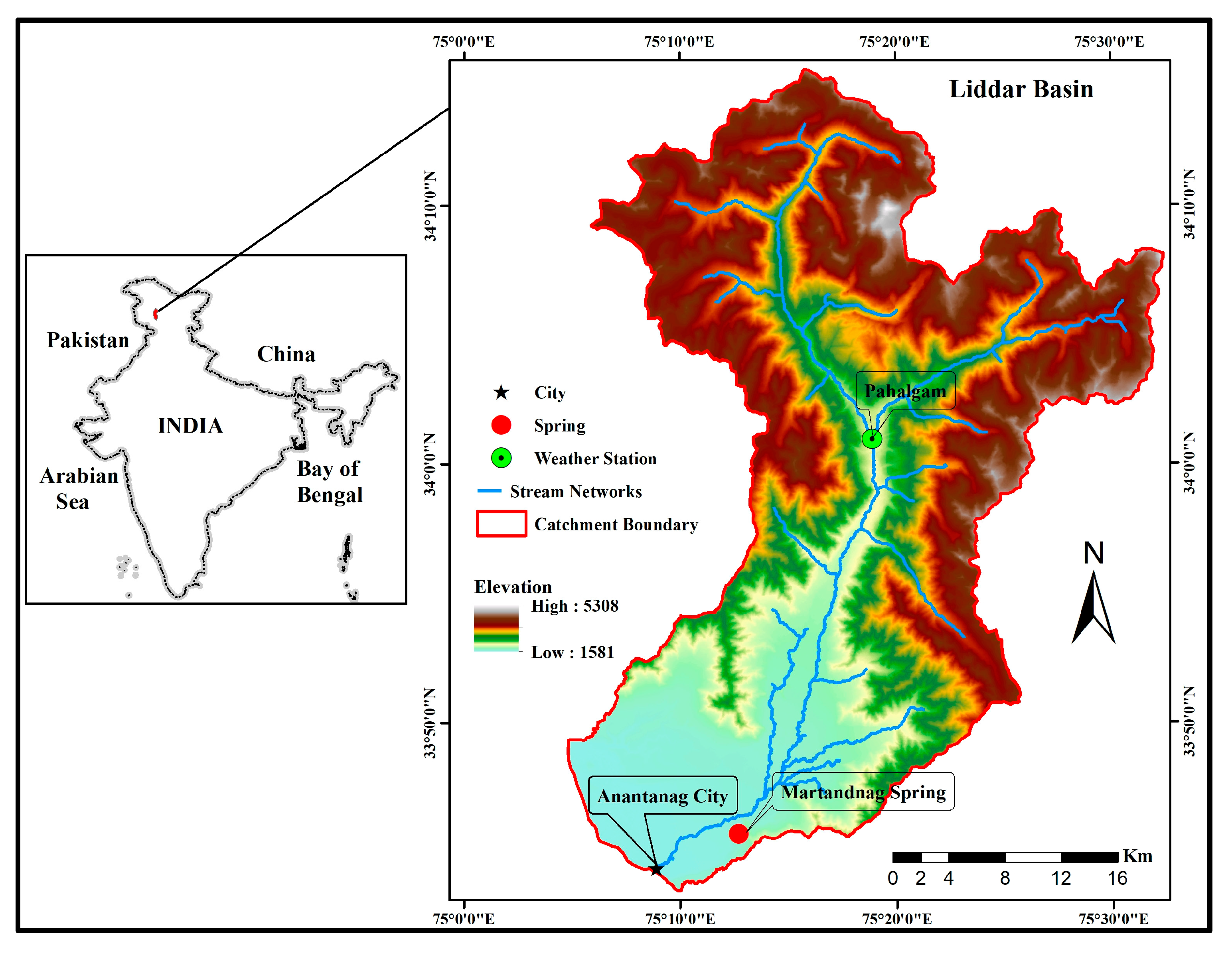
Figure 1. Map showing the location of Martandnag spring in the Liddar basin.
Sustainability 15 08666 g001
Figure 2. Daily time series of stage at Martandnag spring, daily time series of rainfall and air temperature measured at Pahalgam weather station, and monthly time series of snow-covered area (SCA) derived from NDSI. The red rectangle in the uppermost plot denotes the data gap for the spring stage from July 2016 to April 2019.
Sustainability 15 08666 g002
Figure 3. Autocorrelation plots for Martandnag spring for 2013–2016. The black and gray solid lines represent the daily and hourly spring stages, respectively. The horizontal black dashed line at ACF = 0.2 indicates the white-noise threshold. The vertical black dashed lines correspond to lag times at ACF = 0.2.
Sustainability 15 08666 g003
Figure 4. Cross-correlation plots for daily time series over 2013–2016 and 2019–2020. The vertical dashed lines represent the peak response of the spring stage to rainfall and maximum and minimum air temperatures. The associated time lags are noted in the legend for the respective parameters. The horizontal black solid lines represent the statistical significance at 95% confidence intervals.
Sustainability 15 08666 g004
Figure 5. Prediction of monthly Martandnag spring stage in 2030 based on four different IPCC climate change scenarios.
Sustainability 15 08666 g005
Figure 6. Percentage changes in the monthly spring stage in 2030, relative to 2013–2020, based on the IPCC climate change scenarios.
Sustainability 15 08666 g006
Table 1. Sources of data used in the study. Note that data gaps exist for stage data. Rainfall and air temperature data were obtained from IMD; snow-cover data are derived from [33].
Hydrometeorological Data
SiteData TypeUnitsTime ResolutionPeriod
Martandnag spring
Pahalgam
StagemHourly2013–2016, 2019–2020
Rainfall, air temperaturemm, °CDaily2013–2020
Satellite Data
NameNumber of BandsSpatial ResolutionZonePeriod
Landsat 8 OLI/TIRS S2SP1130 mUTM zone 45 N2013–2020
Table 2. Summary statistics for spring stage, rainfall, maximum air temperature (T), minimum air temperature, mean air temperature, and SCA in the Liddar watershed over 2013–2020. All values except SCA are based on daily data; n = number of records.
ParameterMeanStd. ErrorMed.Max.Min.n
Stage (m)2.070.012.053.001.671653
Rainfall (mm)3.640.190115.202424
Max. air T (°C)16.990.1618.5030.3−22424
Min. air T (°C)3.710.143.9020.2−14.72424
Mean air T (°C)10.350.1411.2025.2−7.752424
SCA (km2)211.9018.48156.69613.930121
Table 3. Comparison of RFR and SVR model performances, based on RMSE and R2. Model I comprises all five predictor variables with monthly average data; model II contains daily data for four variables, excluding SCA; model III uses all five predictor variables with daily data. Best-fit model results are denoted in bold.
Random Forest Regression (RFR)
RMSER2
Model I0.10.74
Model II0.190.25
Model III0.170.36
Support Vector Regression (SVR)
Model I—KernelsRMSER2
Linear0.10.6
Polynomial0.080.59
Radial0.060.81
Sigmoid0.170.29
Model II—KernelsRMSER2
Linear0.190.32
Polynomial0.190.3
Radial0.180.35
Sigmoid6.530.14
Model III—KernelsRMSER2
Linear0.180.39
Polynomial0.190.33
Radial0.160.49
Sigmoid5.80.17
Disclaimer/Publisher’s Note: The statements, opinions and data contained in all publications are solely those of the individual author(s) and contributor(s) and not of MDPI and/or the editor(s). MDPI and/or the editor(s) disclaim responsibility for any injury to people or property resulting from any ideas, methods, instructions or products referred to in the content.