Article

Statistical Characteristics of Air Quality Index DAQx*-Specific Air Pollutants Differentiated by Types of Air Quality Monitoring Stations: A Case Study of Seoul, Republic of Korea

1
Department of Urban Climatology, Office for Environmental Protection, City of Stuttgart, D-70182 Stuttgart, Germany
2
Laboratory of Landscape Architecture, Department of Horticultural Science, Faculty of Bioscience and Industry, College of Applied Life Science, Jeju National University, Jeju-si 63243, Republic of Korea
3
Chair of Environmental Meteorology, Albert-Ludwigs-University of Freiburg, D-79085 Freiburg, Germany
*
Author to whom correspondence should be addressed.
Sustainability 2023, 15(11), 8599; https://doi.org/10.3390/su15118599
Submission received: 26 April 2023 / Revised: 18 May 2023 / Accepted: 22 May 2023 / Published: 25 May 2023
(This article belongs to the Special Issue Urban Climate and Health)

Abstract

:
Seoul has a high density of air quality monitoring stations (AQMSs) grouped into roadside, urban, and background types. Using the extensive data from 42 AQMSs in the period 2018 to 2021, the statistical characteristics of air pollutants required to calculate the daily air quality index DAQx* (daily maximum 1 h O3 and NO2 means and daily 24 h PM10 and PM2.5 means) are determined, depending on station types and three temporal periods (individual years, winters, and summers). The results for (i) annual cycles, which include peak concentrations of PM10 (up to 517 µg/m3 in May 2021) and PM2.5 (up to 153 µg/m3 in March 2019) owing to transboundary transport, (ii) annual medians, (iii) annual scattering ranges, (iv) partitioning of frequencies into DAQx*-related concentration ranges, and (v) maximum daily variations within individual station types indicate clear statistical air pollutant characteristics depending on the station types. They were primarily caused by different emission and atmospheric exchange conditions in a circular buffer around each AQMS, which are often approximated by urban form variables. The maximum daily variations were highest in the middle NO2 concentration range of the “satisfying” class for the roadside type (between 53% in summer 2019 and 90% in winter 2020).

1. Introduction

Worldwide urban air quality is often assessed using national limit values for individual air pollutants relevant to human health [1,2,3,4,5,6]. To account for the mix of air pollutants that people breathe, air quality indices (AQIs) have been developed to supplement stand-alone assessments of individual air pollutants, particularly for applications in urban planning and for providing information to the population on the internet about overall air quality [7,8,9,10,11]. The air pollutants recorded over a long term at ground-based air quality monitoring stations (AQMSs) are commonly used for determining AQIs. Assessments of air pollution using AQIs for different AQMS types, which is interesting especially in larger cities, require air pollutant data from comparatively many AQMSs. In this regard, megacities, which often suffer the most from high air pollution and therefore have fundamental adverse impacts on human health, are of particular importance [2,12,13,14].
Historically, air pollution assessments according to individual air pollutants were based only on whether the national limit values were exceeded. However, graded assessments, for which there is a need for various reasons [7,8,9,10,11], are impossible with this method. By contrast, AQIs consider several air pollutants that are hazardous to human health and enable graded assessments through specific concentration ranges. Their breakpoints have been derived from epidemiological and toxicological impact studies [15,16]. The AQIs available thus far differ in temporal references (e.g., hourly, daily, or annually), number and type of included air pollutants, and assignments of concentration ranges of individual air pollutants to index classes. The concentrations of air pollutants required to calculate AQIs depend on emissions, chemical transformation processes in the atmosphere, and atmospheric dispersion and dilution conditions [17,18,19,20,21,22,23,24,25,26,27,28]. They are often approximated by urban form variables in models such as land use regression (LUR) models to predict the spatial distribution of air pollutants [29,30,31,32]. The methodology used to determine AQIs is described in detail in the literature [10,33,34] and is not repeated here.
The daily air quality index DAQx is an AQI that was developed by the Research and Advisory Institute for Hazardous Substances (FoBiG), Freiburg, Southwest Germany, at the beginning of the 21st century [15,35]. To calculate the classes and values of the DAQx, the relationships between air pollution levels and impacts on human well-being and health had to be established using differentially classified ranges of air pollutant concentrations. They were derived from a comprehensive evaluation of the results available in the literature worldwide, which means that the use of the DAQx is not limited based on national boundaries. New secondary assessments in the recent literature on the human toxicity of air pollutants led to a DAQx update by FoBiG in 2020 [16], hereafter referred to as DAQx*. Whereas the DAQx considered daily maximum 1 h ozone (O3), nitrogen dioxide (NO2), and sulfur dioxide (SO2) means, daily highest 8 h moving carbon monoxide (CO) means, and daily 24 h means of particular matter with an aerodynamic diameter < 10 µm (PM10), only the daily maximum 1 h O3 and NO2 means and daily 24 h means of PM10 and PM2.5 are required for calculating DAQx* values. Additionally, graded concentration ranges and breakpoints of the pollutants were adapted based on updated knowledge of their human health impacts (Table 1).
The application of the DAQx* to 42 AQMSs in the megacity of Seoul, which are grouped into three station types, has shown remarkable variations in the frequency of DAQx* values between individual DAQx* classes from 2018 to 2021, both within and between the AQMS types [36]. The corresponding variations in the air pollutants, which are the key factor for the variations in the DAQx* values, are unknown in the DAQx* concentration ranges. To bridge this gap, the present case study analyzes statistical characteristics of the air pollutants for the DAQx* in Seoul during the same period, 2018 to 2021 [34]. This study is not purely statistical in nature because it also takes into account the DAQx* concentration ranges of air pollutants. Thus, it supplements previous statistical studies on characteristics of air pollutants in Seoul [6,14,37,38,39], which are primarily related to annual trends, daily cycles of hourly means, weekly cycles of daily means, and annual cycles of monthly means but not to daily maximum 1 h means. Moreover, they do not sufficiently account for the differences between and within AQMS types. Therefore, the objective of this case study is to identify and quantify the variability in the four DAQx* air pollutants within and between AQMS types. Since they are already the subjects of previous investigations, this study does not address the determination of statistical air pollutant concentrations at individual AQMSs [14,32,38,39] or the model-based creation of maps showing spatial distributions of air pollutant characteristics in Seoul [32,40,41,42].

2. Materials and Methods

Seoul is the capital of the Republic of Korea, has a population of approximately 11 million (as of November 2022), an area of approximately 605 km2 [29,40], and a relatively high level of air pollution [6,14,37,43], which was also confirmed by the DAQx* results in [36]. This is one of the main reasons for the relatively high density of AQMSs operated by the Korea Environment Cooperation in Seoul [44]. The continuous monitoring of air pollution data provides a suitable basis for meeting the objective of this study. In total, 42 AQMSs across Seoul (Figure 1), which had relatively complete time series of the four air pollutants during the study period, were selected.
The AQMSs were previously grouped into roadside (R: 13 AQMSs, Appendix Table A1), urban (U: 24 AQMSs, Table A2), and background (B: 5 AQMSs, Table A3) types [44]. Figure 1 and the elevations of each AQMS above sea level (asl) in Table A1, Table A2 and Table A3 indicate the topography of Seoul, which is located in a basin surrounded by hilly terrain (higher than approximately 500 m asl) and has a western exit from the Han River toward the Yellow Sea.
The urban AQMSs are evenly distributed across the city as they are located in each of Seoul’s 25 administrative districts. Due to insufficient availability of appropriate air pollution data in the period 2018 to 2021, the urban AQMS in the Gangnam-gu district in the south–southeast area of Seoul [45,46] could not be considered in this study. Similarly to the background AQMSs, the urban AQMSs are installed away from major roads on the roofs of public buildings and measure air pollutants at different heights above ground level (agl), minimizing the impacts of the direct surroundings on air pollution [29]. With this monitoring of the general air pollution, the objective of both station types is achieved. The roadside AQMSs are located a few meters from the curbside of main traffic roads in Seoul and are thus affected by adjacent traffic volumes, meaning they record roadside air pollution at approximately 3 m agl but may not reflect impacts from surrounding land use [32]. The specifications of the measuring devices used at the AQMSs in Seoul are listed in Table A4.
Despite the grouping of AQMSs into three types, differences in air pollutant concentrations between AQMSs of the same type are expected because different local characteristics that influence the concentration of air pollutants, such as emission conditions, atmospheric exchange situations, topography, and varying sampling heights, interact at the sites of individual AQMSs. In this context, studies focused on developing models for the prediction of air pollution in specific areas or regions [30,31,32] often use urban form variables such as land use types as proxy variables and the meteorological parameters air temperature, wind speed, wind direction, and precipitation as commonly called control variables. In [31], the authors conclude that the spatial variability of air pollution can be primarily explained by land use environment variables, while the meteorological parameters mainly control its temporal variability. In model studies simulating air pollution in Seoul, spatial distributions of selected land use types in circular zones with radii between 0.5 km and 5.5 km around each urban AQMS were determined [29,47]. They point to a clear variability in the land use areas around each AQMS [48], which can be interpreted as a further reason for the variations in the air pollutant concentrations among AQMSs of the same type.
This study, which extended over a 4-year period from 1 January 2018 to 31 December 2021, could not be started earlier because PM2.5 was continuously monitored at all AQMSs after 1 January 2018. The study period was interesting because it included social distancing periods in Seoul in 2020 and 2021 (Table A5), which were mandated by the government of the Republic of Korea due to the COVID-19 pandemic [49]. The measures taken during these periods [50,51] mainly resulted in traffic reduction [52,53]. However, they did not have the extent of a complete lockdown.
The O3, NO2, PM10, and PM2.5 data from the 42 AQMSs were quality-checked according to previously validated methods [54,55] and subsequently processed for the determination of the DAQx*. An average assessment of ambient air quality, e.g., in terms of mean monthly or annual index values, cannot be achieved by simply averaging the DAQx* values because of the fundamentals and structure of the DAQx*. For example, to determine the long-term air quality index (LAQx), air pollutants partially other than those in DAQx*, including modified graded concentration ranges, must be applied [35,56]. Therefore, this study only refers to daily maximum 1 h O3 and NO2 means and daily 24 h PM10 and PM2.5 means in their specific concentration ranges for DAQx*.

3. Results

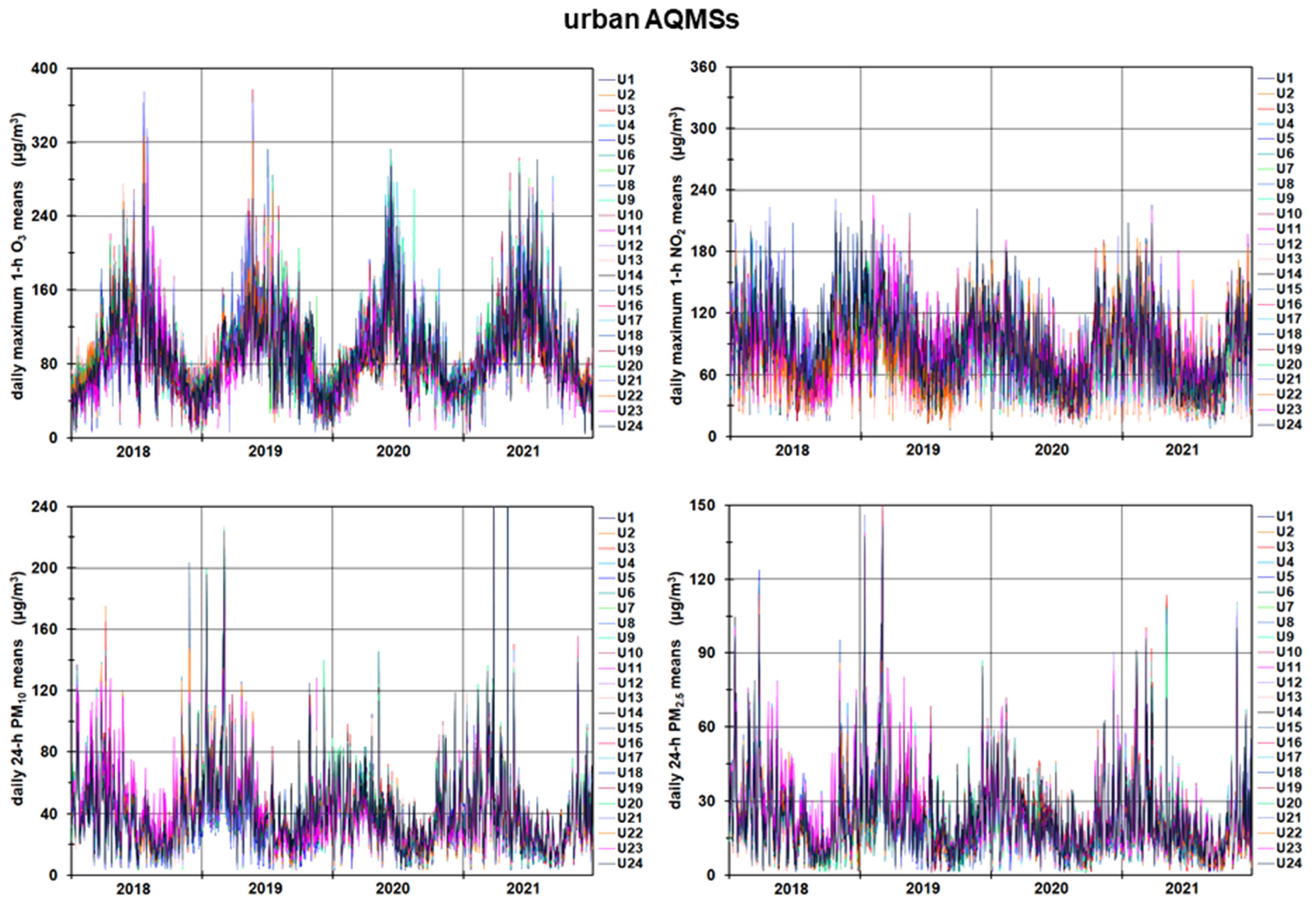
3.1. Annual Cycles of Air Pollutants at AQMSs

The different sources of O3, NO2, PM10, and PM2.5, associated chemical precursors, chemical reactions, and meteorological influences on their concentrations in the ambient air have already been studied in Seoul in many ways [6,14,22,23,25,26,28,29,30,31,32,36,37,38,39,40,42,45,46,47,55,57,58,59,60,61,62,63,64,65,66,67,68,69,70,71,72,73,74]. Therefore, they can be assumed to be known when discussing their annual cycles.
The time series of the daily values of the four air pollutants monitored at individual AQMSs were arranged according to the station types, as shown in Figure 2, Figure 3 and Figure 4. O3, PM10, and PM2.5 displayed recognizable annual cycles for each type of AQMSs, which were the most pronounced for O3. The U type AQMSs showed clear annual cycles of NO2 in all four years, whereas they were weaker for B type and hardly recognizable for R type AQMSs. Additionally, a slightly lower NO2 level was observed in 2020 and 2021 than in 2018 and 2019 mainly because of the traffic reductions during social distancing periods [52,53].
Due to photochemical reactions with precursors, primarily nitrogen oxides and volatile organic compounds [26], in the presence of solar radiation [57], the maximum concentrations of the secondary air pollutant O3 were observed in the summer months, especially in June [69], whereas O3 concentrations were minimal in the winter months. By contrast, the minimum and maximum PM10 and PM2.5 concentrations occurred in the late summer months because of wet scavenging through monsoonal heavy rainfall [70] and in the late winter months, which had less rainy days [36,46]. Extreme values of NO2 were also observed during these months, if an annual cycle could be identified at all, i.e., mainly for the U type AQMSs. Long-range transboundary transport of Asian dust because of air flow from western directions during specific synoptic conditions [22,23,25,59,67,75,76] led to severe PM episodes of up to three consecutive days with extremely high concentrations of PM10 (up to 517 µg/m3 on 8 May 2021) and PM2.5 (up to 153 µg/m3 on 5 March 2019).
Although the number of AQMSs grouped into the three types is different (Table A1, Table A2 and Table A3), Figure 2, Figure 3 and Figure 4 indicate remarkable variations in the air pollutant concentrations monitored at AQMSs within the same station type. They are also reflected to some extent in the medians of the air pollutant time series over the entire study period (Table A1, Table A2 and Table A3).
With regard to an additional structuring of the results in Figure 2, Figure 3 and Figure 4, it is pointed out that in [36], the daily values of the four air pollutants are aggregated into monthly mean values per station type for each year in the study period.

3.2. Annual Air Pollutant Medians per AQMS Type

The annual medians of the daily maximum 1 h O3 means for all AQMSs per station type showed an increasing tendency from 2018 to 2021 (Table 2), which amounted to 12 µg/m3 for the R, 10 µg/m3 for the U, and 20 µg/m3 for the B types. By contrast, similar medians of the daily maximum 1 h NO2, daily 24 h PM10, and daily 24 h PM2.5 means were characterized by a decreasing tendency in the same period, which was related to the NO2 values, 19 µg/m3 for the R and 15 µg/m3 for the U and B types. The decrease in the annual PM10 medians was the highest (9 µg/m3) for the R type and lowest (6 µg/m3) for the other two types. The decreasing tendency of annual PM2.5 medians was only marginally higher for both the R and U types (4 µg/m3) than for the B type (3 µg/m3).
The annual medians of the daily maximum 1 h O3 means was the highest for the B type (“satisfying” class according to Table 1) and lowest for the R type (“good” class), with a mean difference of 24 µg/m3 between both types. In contrast, the annual medians of the daily maximum 1 h NO2, daily 24 h PM10, and daily 24 h PM2.5 means were the highest for the R type (for NO2: “sufficient” class in 2018 and 2019, “satisfying” class in 2020 and 2021; for PM10: “sufficient” class in 2018, “satisfying” class from 2019 to 2021; for PM2.5: “satisfying” class in 2018 and 2019, “good” class in 2020 and 2021) and lowest for the B type (for NO2 and PM10: “satisfying” class from 2018 to 2021; for PM2.5: “good” class from 2018 to 2021). The mean differences between both types during the study period were 46 µg/m3 for NO2, 6 µg/m3 for PM10, and 3 µg/m3 for PM2.5.

3.3. Annual Scattering Ranges of Air Pollutants per AQMS Type

The extent of the annual scattering ranges in the air pollutant time series for each station type was approximated by the differences between their 0.95 and the 0.05 quantiles (Table 3). During the 4-year study period, the patterns of the annual scattering ranges of the daily maximum 1 h O3, daily 24 h PM10, and 24 h PM2.5 means were almost irregular for each station type, whereas those for the daily maximum 1 h NO2 means showed a slight decrease for all station types from 2018 to 2021. For the daily maximum 1 h O3 means, the annual scattering ranges were the highest for U and lowest for R types with a mean difference of 18 µg/m3. In contrast, the highest annual scattering ranges of the daily maximum 1 h NO2 and daily 24 h PM10 means were observed for the R type, while the lowest ranges were found for the B type with a mean difference of 4 µg/m3 for NO2 and 7 µg/m3 for PM10.

3.4. Frequencies of DAQx*-Relevant Air Pollutants per AQMS Type

The relative frequencies of the DAQx*-relevant air pollutant concentrations per station type (Figure 5, Figure 6, Figure 7 and Figure 8) refer to gradations related to human health, as shown in Table 1, rather than to equidistant, impact-independent gradations of concentration ranges, which are usually applied in statistical air pollution investigations [1,58,73]. In addition to individual years, the graded frequencies were also determined for winter (January–March) and summer (July–September) periods to facilitate an analysis of extreme air pollutant conditions.

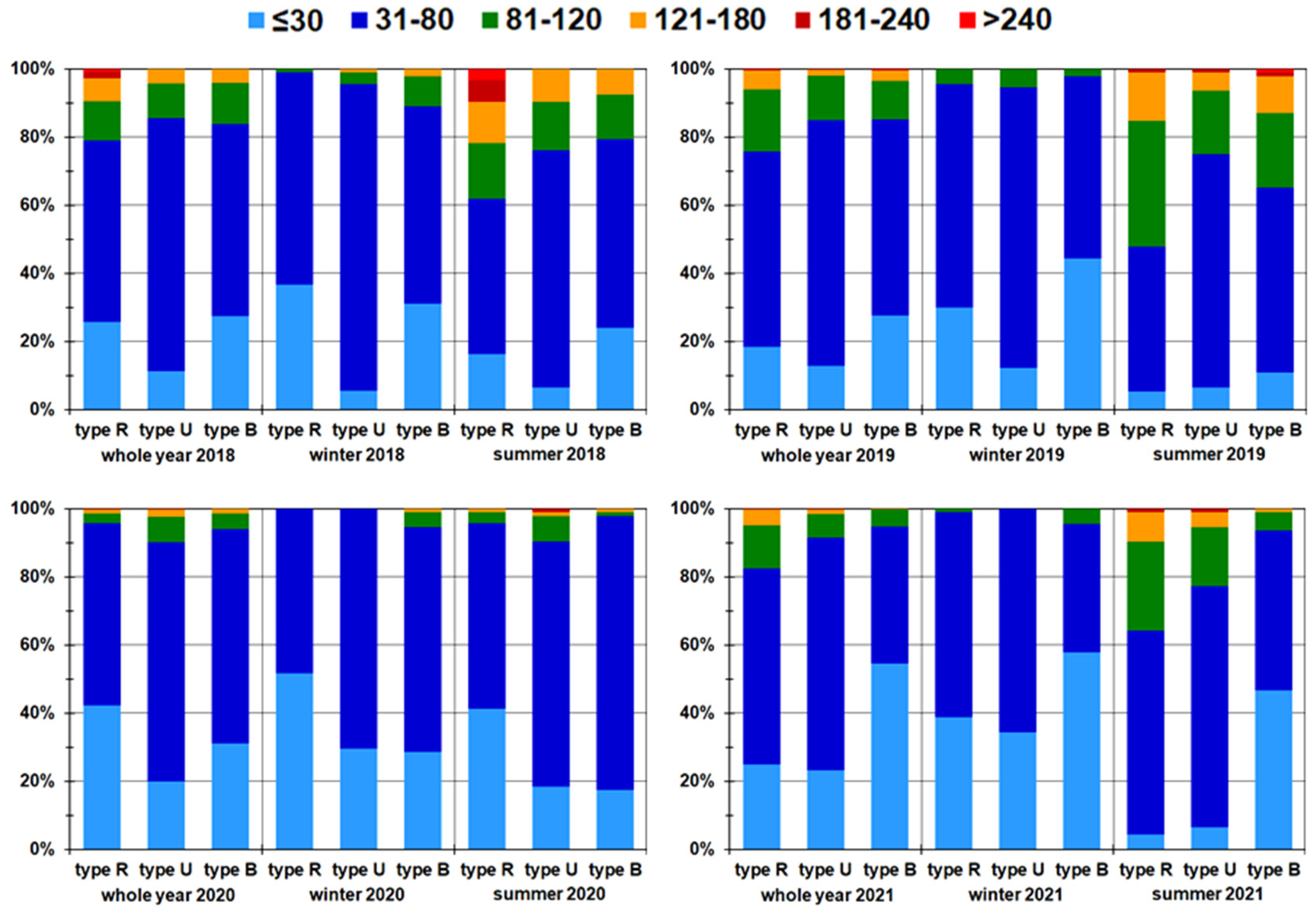
3.4.1. Frequencies of Daily Maximum 1 h O3 Means

In all four study years, the frequencies of the daily maximum 1 h O3 means (Figure 5) were the highest in the “good” class for the R and U types (R type: between 54% in 2021 and 60% in 2018; U type: between 38% in 2021 and 49% in 2020), followed by the “satisfying” class (R type: between 18% in 2018 and 28% in 2021; U type: between 28% in 2018 and 35% in 2019). For the B type, the frequencies of the daily maximum 1 h O3 means in the years 2018 to 2020 were also the highest in the “good” class (between 40% in 2019 and 45% in 2018), followed by the “satisfying” class (between 31% in 2018 and 2019 and 36% in 2020). However, in 2021, the frequencies were the highest in the “satisfying” class (38%) and second highest in the “good” class (28%).
Figure 5. Relative frequencies of the daily maximum 1 h O3 means, grouped according to the concentration ranges (µg/m3) in Table 1, for the three types (R, U, and B) of AQMSs in Seoul from 2018 to 2021 (winter: January to March; summer: July to September).
Sustainability 15 08599 g005
The frequencies in winters were the highest for all station types in the same classes as for the individual years. The R and U types had the highest frequencies in the “good” class (R type: each 73%; U type: between 59% in 2019 and 70% in 2020). The B type had the highest frequencies in the winter periods from 2018 to 2020 in the “good” class (between 52% in 2020 and 59% in 2018) and in winter 2021 in the “satisfying” (44%) class. For the R type, the highest frequencies in the summer periods from 2018 to 2020 were observed in the “good” class (between 48% in 2019 and 59% in 2020) and in summer 2021 in the “satisfying” (41%) class. The U type had the highest frequencies in summer 2018 (35%) and 2021 (42%) in the “satisfying” class, in summer 2019 in the “sufficient” class (34%), and in summer 2020 in the “good” class (42%). In winters, the summed-up frequencies of the “poor” and “very poor” classes were lower than 1%, whereas they reached 4% for R, 10% for U, and 13% for B types in summers.

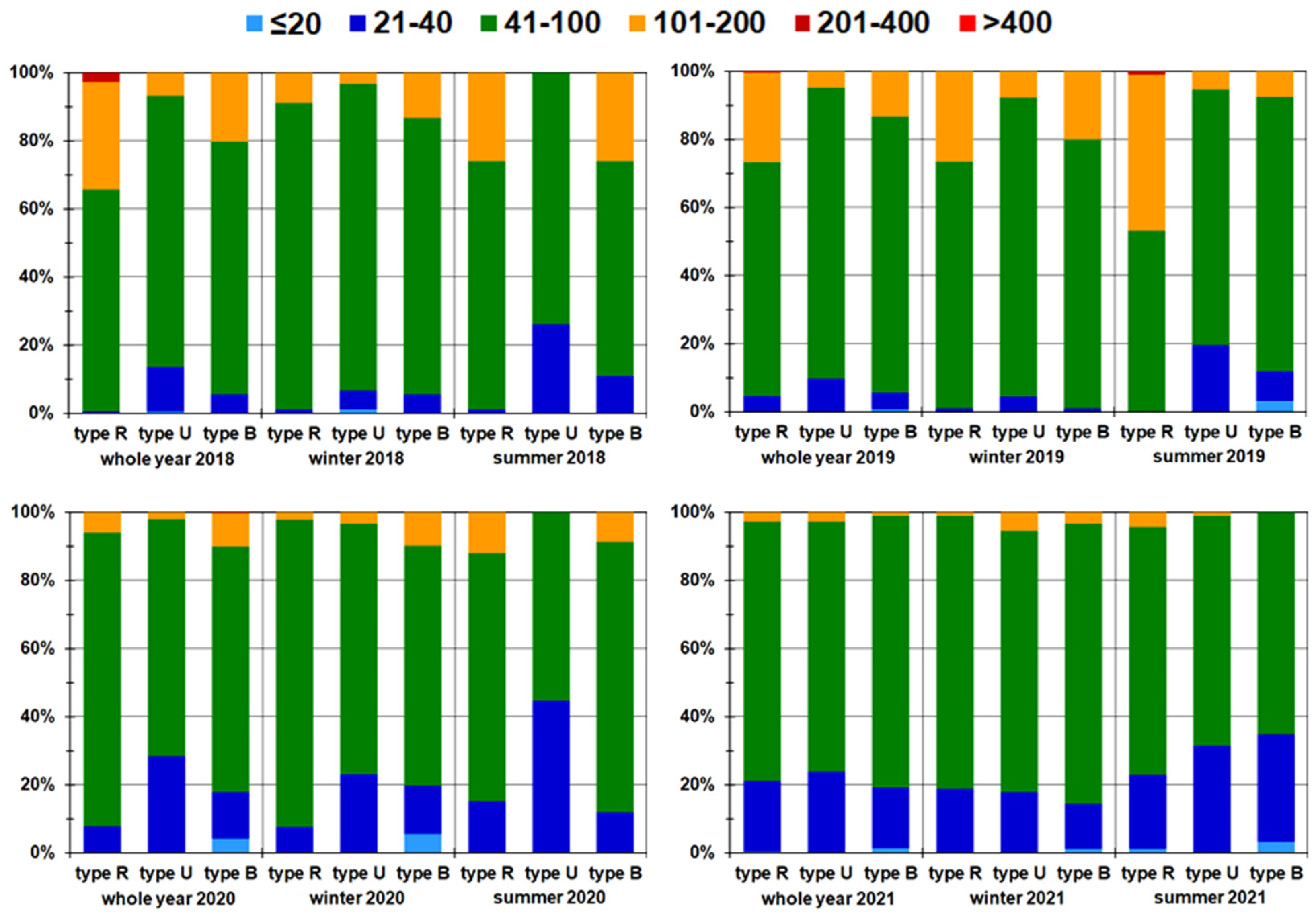
3.4.2. Frequencies of Daily Maximum 1 h NO2 Means

The frequencies of the daily maximum 1 h NO2 means (Figure 6) for the R type were the highest in the “sufficient” class in 2018 (62%) and 2019 (63%) and in the “satisfying” class in 2020 (56%) and 2021 (51%). The NO2 frequencies for both the U and B types were the highest in the “satisfying” class for all study years (U type: between 59% in 2019 and 64% in 2020; B type: between 48% in 2018 and 56% in 2020). The second-highest frequencies for the R type were observed in the “satisfying” class in 2018 and 2019 (each 34%) and “sufficient” class in 2020 (42%) and 2021 (47%). The second-highest frequencies for the U type occurred in the “sufficient” class in each study year (between 22% in 2020 and 33% in 2019). The B type had the second-highest frequencies in 2018 (26%) and 2019 (21%) in the “sufficient” class and in 2020 (24%) and 2021 (27%) in the “good” class.
Figure 6. Relative frequencies of the daily maximum 1 h NO2 means, grouped according to the concentration ranges (µg/m3) in Table 1, for the three types (R, U, and B) of AQMSs in Seoul from 2018 to 2021 (winter: January to March; summer: July to September).
Sustainability 15 08599 g006
For the R type, the frequencies in winters were the highest in the “sufficient” class for all study years (between 56% in winter 2020 and 77% in winter 2019). The U type had the highest frequencies in the “sufficient” class in winter 2018 (53%) and 2019 (60%) and in the “satisfying” class in winter 2020 (57%) and 2021 (51%). In each of the four winter periods, the B type had the highest frequencies in the “satisfying” class (between 47% in 2019 and 62% in 2020). The highest frequencies during all summer periods were observed in the “satisfying” class for all station types (R type: between 49% in 2019 and 76% in 2020; U type: between 65% in 2020 and 80% in 2018; B type: between 36% in 2019 and 56% in 2020). The summed-up frequencies of the daily maximum 1 h NO2 means for the R type in both the “poor” and “very poor” classes was lower than 4% during the entire study period (2% in winters and 3% in summers), and the comparable frequencies of the U and B types were even lower.

3.4.3. Frequencies of Daily 24 h PM10 Means

The frequencies of the daily 24 h PM10 means for the R type (Figure 7) were the highest in the “satisfying” class (between 24% in 2018 and 31% in 2020) for all study years. The U type had the highest frequencies in the “satisfying” class in the years 2018 to 2020 (between 27% in 2018 and 30% in 2020) and even in the “good” class in 2021 (32%). The B type had the highest frequencies in the “satisfying” class in 2018 (28%) and 2019 (33%) and in the “good” class in 2020 (30%) and 2021 (34%). The second-highest frequencies for the R type were observed in the “poor” class from 2018 to 2020 (between 21% in 2019 and 24% in 2018) and in the “good” class in 2021 (28%). The U type had the second-highest frequencies in the “good” class from 2018 to 2020 (between 23% in 2019 and 28% in 2020) and in the “satisfying” class in 2021 (29%). The B type had the second-highest frequencies in the “good” class in 2018 (26%) and 2019 (24%) and in the “satisfying” class in 2020 (26%) and 2021 (27%).
Figure 7. Relative frequencies of the daily 24 h PM10 means, grouped according to the concentration ranges (µg/m3) in Table 1, for the three types (R, U, and B) of AQMSs in Seoul from 2018 to 2021 (winter: January to March; summer: July to September).
Sustainability 15 08599 g007
The highest frequencies for both R and U types occurred in winters from 2018 to 2020 in the “poor” class (R type: 35% in both 2018 and 2019 and 39% in 2020; U type: between 31% in 2018 and 32% in 2020) and in winter 2021 in the “satisfying” class (R type: 25%; U type: 26%). The highest frequencies for the B type were observed in winter 2018 (27%) and 2019 (30%) in the “poor” class and in winter 2020 (28%) and 2021 (26%) in the “satisfying” class. The highest frequencies for all station types in summers were observed in the “good” class (R type: between 41% in 2018 and 52% in 2021; U type: between 48% in 2018 and 54% in 2021; B type: between 43% in 2019 and 51% in 2021).
For each individual year, winter, and summer, the summed-up frequencies of the daily 24 h PM10 means for the classes “poor” and “very poor” were always the highest for the R type, whereas a decreasing tendency for the B type was observed. The annual frequencies for the R type were the highest in 2018 (37%), for the U type in 2019 (27%), and for the B type in 2018 and 2019 (each 23%). The highest frequencies for each of the three types in winter (R type: 62%; U type: 58%; B type: 51%) and summer (R type: 4%; U and B types: each 3%) were observed in 2019.

3.4.4. Frequencies of Daily 24 h PM2.5 Means

The frequencies of the daily 24 h PM2.5 means for each individual year (Figure 8) were the highest in the “good” class for all station types (R and U types: both between 35% in 2018 and 46% in 2021; B type: between 41% in 2020 and 47% in 2019). The second-highest frequencies for the R type were observed in the “satisfying” class (between 18% in 2021 and 24% in 2019). This class also showed the second-highest frequencies for the U type from 2018 to 2020 (between 21% in 2018 and 23% in 2019), whereas the “very good” class showed the second-highest frequencies in 2021 (18%). The B type had the second-highest frequencies in the “satisfying” class in 2018 and 2019 (each 22%) and in the “very good” class in 2020 and 2021 (each 23%).
Figure 8. Relative frequencies of the daily 24 h PM2.5 means, grouped according to the concentration ranges (µg/m3) in Table 1, for the three types (R, U, and B) of AQMSs in Seoul from 2018 to 2021 (winter: January to March; summer: July to September).
Sustainability 15 08599 g008
The highest frequencies for all the three station types in winters were observed in the “good” class (R type: between 26% in 2019 and 41% in 2021; U type: between 27% in 2019 and 41% in 2021; B type: between 29% in 2019 and 42% in 2021). During summers, the “good” class showed the highest frequencies for both the R and U types (R type: between 47% in 2021 and 52% in 2018; U type: between 47% in 2020 and 2021 and 50% in 2019). The highest frequencies for the B type in summers also occurred in the “good” class in 2018 (50%) and 2019 (51%) and in the “very good” class in 2020 (52%) and 2021 (51%).
For each individual year, winter, and summer, the summed-up frequencies of the daily 24 h PM2.5 means for the classes “poor” and “very poor” were always the highest in the year 2019, whereas a decreasing tendency, particularly in individual years and winters, from the R to B types was observed. The frequencies in the whole year of 2019 were 20% for the R type, 18% for the U type, and 12% for the B type. The frequencies in winter 2019 were 42% for the R type, 41% for the U type, and 31% for the B type, whereas they were 5% for both the R and B types and 4% for the U type in summer 2019.

3.5. Variations of DAQx*-Relevant Air Pollutants within AQMS Types

The variations in the annual cycles of the DAQx*-relevant air pollutants at AQMSs, which are evident in Figure 2, Figure 3 and Figure 4 for the three station types, were mainly caused by their locations within various land use types and specific sampling heights, resulting in locally different emissions and air exchange conditions. The daily variations of the DAQx*-relevant air pollutants per station type were quantified using the maximum differences between all AQMSs of the same station type. From the two possibilities for grouping the variation results in the form of frequencies, namely, equidistant or impact-related grouping according to Table 1, the second variant, which allowed a graded assessment because of the DAQx* reference, was chosen (Figure 9, Figure 10, Figure 11 and Figure 12).

3.5.1. Variations of Daily Maximum 1 h O3 Means

For each individual year, winter, and summer, the variations of the daily maximum 1 h O3 means in terms of frequencies were the highest (between 42% in summer 2019 for the R type and 90% in winter 2018 for the U type) in the concentration range of the “good” class (Figure 9) within all station types. Only in the whole year 2021 (B type: 55%) and in winter 2020 (R type: 52%) and 2021 (B type: 58%), the frequencies dominated in the lower concentration range of the “very good” class. Except for summer 2019 and 2021, the second-highest frequencies were always in the concentration range of the “very good” class. Among the three station types, the frequencies of the U type in the concentration range of the “good” class were the highest (more than 65%) in all temporal periods. Apart from a few exceptions, the frequencies in this class were the lowest for the R type. Overall, the frequencies characterizing the variations within the station types were limited to concentration ranges from “very good” to “sufficient” classes. In the concentration range of the “sufficient” class, the frequencies generally did not exceed 10%, except for 14% in summer 2019 for the R type.
Figure 9. Relative frequencies (%) of the maximum differences of the daily maximum 1 h O3 means between all AQMSs of the same station type (R, U, and B), grouped according to the concentration ranges (µg/m3) in Table 1, in Seoul from 2018 to 2021 (winter: January to March; summer: July to September).
Sustainability 15 08599 g009

3.5.2. Variations of Daily Maximum 1 h NO2 Means

The highest variations of the daily maximum 1 h NO2 means (between 53% in summer 2019 and 90% in winter 2020, both for the R type) were observed in all temporal periods and for all station types in the concentration range of the “satisfying” class (Figure 10), showing the tendency of higher frequencies in winters than in summers. The pattern of the second-highest variations of NO2 was not as clear as that of O3. For NO2, the frequencies were mostly in the concentration range of the “sufficient” class. No frequencies in the low NO2 concentration range of the “very good” class compared to those of O3 were observed for any station type. Identifying a station type with the highest frequencies in the concentration range of the “satisfying” class in each temporal period was also not possible. The variations of NO2 within each station type were lower in the concentration range of the “good” class (maximum: 45% in summer 2020 for the U type) than those of O3 (minimum: 46% in summer 2018 for the R type). However, they were higher in the concentration range of the “satisfying” class (minimum: 53% in summer 2019 for the R type) than those of O3 (maximum: 37% in summer 2019 for the R type).
Figure 10. Relative frequencies (%) of the maximum differences of the daily maximum 1 h NO2 means between all AQMSs of the same station type (R type: roadside, U type: urban, B type: background), grouped according to the concentration ranges (µg/m3) in Table 1, in Seoul from 2018 to 2021 (winter: January to March; summer: July to September).
Sustainability 15 08599 g010

3.5.3. Variations of Daily 24 h PM10 Means

The variations of the daily 24 h PM10 means in the individual study years (Figure 11) were the most pronounced in the concentration range of the “good” class for the R (between 51% in 2020 and 68% in 2019) and U (between 48% in 2021 and 66% in 2019) types but in the “very good” class for the B type in 2018 (43%), 2020 (49%), and 2021 (55%). The frequencies for all station types in winters were also the highest in the concentration range of the “good” class (between 41% in winter 2018 for the B type and 70% in winter 2019 for the R type). In summers, both the R and U types tended to have the highest frequencies in the concentration range of the “good” class (R type: between 64% in summer 2019 and 74% in summer 2018; U type: between 63% in summer 2020 and 70% in summer 2019) and the B type in the concentration range of the “very good” class (between 72% in summer 2018 and 82% in summer 2021). None of the station types showed the highest frequencies per year during all temporal periods. As for NO2, no type-specific concentration range could be found for PM10 that clearly had the second-highest frequencies in all periods. The variations of the daily 24 h PM10 means within each station type were observed in the concentration ranges of the classes “very good” to “very poor” for individual years and winters, with frequencies decreasing below 6% in the classes “sufficient” to “very poor”. However, these variations were only observed in the concentration ranges of the classes “very good” to “satisfying” in summers.
Figure 11. Relative frequencies (%) of the maximum differences of the daily 24 h PM10 means between all AQMSs of the same station type (R type: roadside, U type: urban, B type: background), grouped according to the concentration ranges (µg/m3) in Table 1, in Seoul from 2018 to 2021 (winter: January to March; summer: July to September).
Sustainability 15 08599 g011

3.5.4. Variations of Daily 24 h PM2.5 Means

The most frequent variations of the daily 24 h PM2.5 means in the R (above 54%) and U (above 57%) types were observed in the concentration range of the “good” class (Figure 12) from 2018 to 2020 and in the lower concentration range of the “very good” class (R type: 63%; U type: 48%) in 2021. In each of the four study years, the B type always showed the most frequent variations in the concentration range of the “very good” class (between 54% in 2020 and 73% in 2021).
Figure 12. Relative frequencies (%) of the maximum differences of the daily 24 h PM2.5 means between all AQMSs of the same station type (R type: roadside, U type: urban, B type: background), grouped according to the concentration ranges (µg/m3) in Table 1, in Seoul from 2018 to 2021 (winter: January to March; summer: July to September).
Sustainability 15 08599 g012
This specific pattern for each station type was also evident in winter 2018 and 2019. However, in winter 2020, the most frequent variations of the daily 24 h PM2.5 means in the B type were found in the “good” class concentration range (50%), whereas in winter 2021, the variations in the R and B types were the most frequent in the concentration range of the “very good” class (R type: 48%; B type: 51%) and in the U type in the concentration range of the “good” class (49%).
All station types showed the tendency of the most frequent variations in the concentration range of the “very good” class (above 57%) in summers, except for the R type in summer 2019 and 2020 and the U type in summer 2018 and 2019, in which the most frequent variations were in the concentration range of the “good” class (above 51% for the R type and 66% for the U type). However, none of the station types showed the most frequent variations in all individual study years and winters, although the B type always had the most frequent variations in summers (between 72% in 2020 and 94% in 2018).
The variations of the daily 24 h PM2.5 means for the R and U types during all temporal periods were distinctly lower in the concentration ranges of the “satisfying” class (below 17%) than those in the lower concentration ranges of the “good” and “very good” classes. The PM2.5 variations in summer 2018 and 2021 were observed only in the concentration ranges of the “good” and “very good” classes, whereas they also covered the concentration range of the “satisfying” class in summer 2019 and 2020. The PM2.5 variations throughout 2019 and winter 2019 were observed in all six classes.

3.6. Social Distancing Effects

The measures imposed in Seoul during social distancing periods owing to the COVID-19 pandemic have mainly led to reduced traffic-dependent air pollution [77,78]. The corresponding statistical studies, which are based on monitored air pollutant concentrations, mostly relate to the stronger social distancing period in the first half of 2020 (Table A5). Their results are summarized in [36]. In another study, concentration changes in daily maximum 1 h O3 and NO2 means, and daily 24 h PM10 and PM2.5 means, each averaged over the stronger social distancing period from 19 August to 11 October 2020, were analyzed based on air pollution data monitored at the same AQMSs as in this study [36].
Taking into account different intensity levels, the social distancing periods in Seoul extended almost completely over the years 2020 and 2021 (Table A5). As a result, the concentration levels of the annual medians averaged over 2020 and 2021 were lower by about 17% for daily maximum 1 h NO2 means, 14% for daily 24 h PM10 means, and 15% for daily 24 h PM2.5 means than those averaged over 2018 and 2019. However, the annual medians for daily maximum 1 h O3 means were higher particularly for the R type in 2020 and 2021 than those in 2018 and 2019 (by about 13%). The annual NO2 scattering ranges were also lower in 2020 and 2021, by about 17% for the R type, 5% for the U type, and 18% for the B type. However, the effects of the traffic reductions did not reach a magnitude large enough to detect systematic changes in the annual variations of the daily maximum 1 h O3 and NO2 means and the daily 24 h PM10 and PM2.5 means within each station type, since the ranges of the different concentration classes were perhaps too wide.

4. Discussion

This study was inspired by a previous investigation on the variability of the recently updated daily air quality index DAQx* in Seoul from 2018 to 2021 [36], which quantified remarkable differences in graded air pollution assessments not only among but also within three types of AQMSs in whole individual years, winters, and summers. Seoul was a well-suited study site because of its relatively high density of AQMSs. A total of 42 AQMSs, grouped into roadside (R: 13 AQMSs), urban (U: 24 AQMSs), and background (B: 5 AQMSs) types, had been selected due to their comparatively complete time series of air pollutants necessary for the determination of DAQx*. To achieve a deeper understanding of the variations in the DAQx* among and within the station types than that in [36], this study aims at analyzing statistical characteristics of air pollutants required for the determination of the DAQx* for the same temporal periods, AQMSs, and types of AQMSs.
Previous statistical studies on air pollution conditions in Seoul were often impact-independent, mostly included daily, monthly, or annual mean values of various air pollutants, and the differences between the types of AQMSs were not addressed in detail [6,14,37,38,39,58,73]. In contrast, this study considers the level of human health impairment owing to air pollution using specific temporal references of the input air pollutants for the DAQx* (daily maximum 1 h O3 and NO2 means, daily 24 h PM10 and PM2.5 means) and human health-related gradations of their concentration ranges. Despite an extensive literature search, no similar studies could be found. Therefore, the discussion of the results is limited to this study itself.
The different results confirmed the relatively high level of air pollution in the topographically heterogeneous area of Seoul, as reported in other studies [14,36,37,38,39,40]. Annual cycles of the four DAQx*-relevant air pollutants monitored at AQMSs of the same type were similar to those in previous studies, although distinctly higher levels of daily maximum 1 h O3 and NO2 means compared to those of their otherwise-presented daily means were shown in the present study. The annual medians of the daily maximum 1 h O3 means were approximately 53% higher for the R type and approximately 64% higher for the U and B types compared to the otherwise usual annual O3 medians, regardless of the station type. The annual medians of the daily maximum 1 h NO2 means were approximately 79% higher for the R type, 71% higher for the U type, and 63% higher for the B type compared to the type-independent annual means [38].
Annual maxima and minima of O3 were observed in summers and winters, respectively, whereas maxima and minima of NO2, PM10, and PM2.5 were found in winters and summers, respectively. In addition to individual study years, these seasonal patterns explained why DAQx*-relevant air pollutants were also analyzed during specific winter (January to March) and summer (July to September) periods. In each study year, extremely high daily 24 h PM10 and PM2.5 means (PM10: up to 517 µg/m3 on 8 May 2021; PM2.5: up to 153 µg/m3 on 5 March 2019) were observed irregularly during severe PM episodes (daily 24 h PM10 means >100 µg/m3; daily 24 h PM2.5 means >35 µg/m3) of up to three days, which resulted from transboundary dust transport [22,23,25,59,67,75,76,79]. Therefore, they were noticeable almost simultaneously at all AQMSs with different intensities. These peak means were responsible for extremely poor air pollution assessments by the DAQx* (DAQx* > 10) [36], indicating extremely high short-term risks to human health.
Annual medians for all AQMSs over the entire study period and annual medians for the types of AQMSs in individual years structured the results for the annual cycles of air pollutants. The annual medians of the daily maximum 1 h O3 means tended to be highest for the B type and lowest for the R type, whereas the annual medians of the daily maximum 1 h NO2, daily 24 h PM10, and daily 24 h PM2.5 means were the highest for the R type and lowest for the B type. As the study period covered only four years, including the last two years with social distancing periods, it was not surprising that temporal trends of the analyzed air pollutants could not be determined for all station types, also because the dependencies of air pollutant concentrations on emission and air exchange conditions cannot be separated in a simple way [18]. Only increasing tendencies of O3 for the R type and decreasing tendencies of NO2 for the B type, PM10 for all types, and PM2.5 for both the U and B types were identified.
Annual scattering ranges of air pollutants per station type were approximated by differences between the 0.95 and 0.05 quantiles of their annual time series. The scattering ranges in the complete study period averaged over the three station types were the highest for the daily maximum 1 h O3 means (137 µg/m3, corresponding to 100%). The comparable scattering ranges were 84% for the daily maximum 1 h NO2 means, 53% for the daily 24 h PM10 means, and 32% for the daily 24 h PM2.5 means. According to the types of AQMSs, the annual scattering range of O3 from 2018 to 2021 was the highest for the B type (146 µg/m3, corresponding to 100%), whereas it was 97% for the U type and 85% for the R type. The comparable scattering range of NO2 was the highest (119 µg/m3, corresponding to 100%) for the R type, whereas it was 94% for the U type and 97% for the B type. PM10 also showed the highest scattering range for the R type (76 µg/m3, corresponding to 100%), whereas it was 95% for the U type and 91% for the B type. The highest scattering range for PM2.5 was also observed for the R type (46 µg/m3, corresponding to 100%), whereas it was 99% for the U type and 87% for the B type. The difference in the magnitude of the scattering ranges between the air pollutants was not only caused by the individual location of the AQMSs and their surrounding land use types but also by the different residence times of the air pollutants in the ambient air, which were approximately 1 h for O3, 4 h for NO2, and days to weeks for PM10 and PM2.5 [2,27,74], and other air chemical characteristics, such as chemical reactions for O3 and NO2 and deposition processes for PM10 and PM2.5.
The frequencies of the specific daily means of the air pollutants in their concentration ranges, which were graded according to their human health impact (Table 1), indicated their differential seasonal risk potentials. In addition to the extent of average impairments of human health, which was reflected by the concentration ranges with the highest frequencies, the frequencies summed up over the “poor” and “very poor” classes were of particular importance because they point out peak exposures to human health. For O3, they mainly occurred in summer in the U (10%) and B (13%) types. Almost independent of the temporal study periods, they were determined for NO2 only in the R type, although to a lesser extent (no more than 4%) than those for O3 in summer. For PM10 and PM2.5, the summed-up frequencies for the “poor” and “very poor” classes in the individual years, but especially in winter, were significantly higher than those for O3 or NO2. These were 62% for PM10 and 20% for PM2.5 in winter 2019 for the R type. A trend toward higher frequencies for PM10 than for PM2.5 and a decrease in their frequencies from the R to B types was observed. Overall, over the study period, the extreme health hazards from air pollution in Seoul that could be quantified using DAQx* [36] were mainly caused by PM10 and PM2.5 in winter and to a lesser extent by O3 in summer.
Regardless of the number of AQMSs for each station type, the expected impact-related variations in air pollutant concentrations within the station types, which were evident in the annual cycles of the four air pollutants, could be quantified. These variations were caused by the interaction of local effects of emissions, chemical reactions in the ambient air, transboundary transport, air exchange conditions, topography, and sampling heights because these commonly called independent variables determined the concentrations of air pollutants as dependent variables at the individual AQMSs. As shown in [48], for circular 1 km buffers around each of 7 roadside, 25 urban, and 2 background AQMSs in Seoul, the spatial extent of these independent variables, for which GIS land uses are often used as proxy variables, differs between the AQMSs, sometimes significantly. The variations of O3, PM10, and PM2.5 according to the station types were frequently most pronounced in the concentration range of the “good” class (O3: between 42% in summer 2019 for the R type and 90% in winter 2018 for the U type; PM10: between 41% in winter 2018 for the B type and 74% in summer 2018 for the R type; PM2.5: between 46% in winter 2018 for the U type and 74% throughout 2020 for the R type). In contrast, the concentration range of the “satisfying” class showed the most common NO2 variations (between 53% in summer 2019 and 90% in winter 2020, each for the R type). Collectively, the variations of air pollutants per station type most often occurred in the concentration ranges from the “very good” to “sufficient” classes for O3 and the “good” to “sufficient” classes for NO2. However, the variations of PM10 and PM2.5 per station type extended to the entire concentration range from the “very good” to “very poor” classes. Overall, the variations in the DAQx*-relevant air pollutants within the station types reached impact-related levels, particularly for NO2, which were previously unknown. The occurrence of lower frequencies in the “poor” and “very poor” classes for PM10 and PM2.5 reflect their broader variations. The results reported in this study will help to understand the variations of the DAQx* in a clearer way compared to those in the prior study [36].
Although the intensity of the “social distancing policy” measures in Seoul did not reach the level of a complete lockdown in 2020 and 2021, effects mainly of vehicular traffic reductions [52] on the concentrations of the DAQx*-relevant air pollutants could be detected, even if not only individual stronger social distancing periods were taken as a basis but the years 2020 and 2021 as a whole compared to the previous years 2018 and 2019. Reductions in traffic density in 2020 and 2021 resulted in desirable lower concentrations of the DAQx*-relevant air pollutants that depend on traffic, primarily NO2. However, this was associated with the disadvantage of higher O3 concentrations, which increased the human health risk, especially when there was high solar radiation in summer [26,57].

5. Conclusions

Referring to a prior study on the human health-related assessment of air pollution in Seoul using the air quality index DAQx* [36], this study focused on examining statistical characteristics of air pollutants monitored at 42 AQMSs in Seoul. The results, which are crucial for understanding the variations in the DAQx*, include the quantification of the dependence of annual cycles of air pollutants, annual air pollutant medians, annual scattering ranges of air pollutants, and frequencies of DAQx*-relevant air pollutants for the three types into which AQMSs in Seoul are grouped. However, this study is not a conventional statistical study on air pollutant indicators because the basis and structure of the DAQx* dictated the temporal references of the specific air pollutants and their graded impact-related concentration ranges. Therefore, this study, which covers three temporal periods (individual years, winters, and summers) from 2018 to 2021, obtained air pollution results for AQMS types that have not been reported to date. However, to make the results even more reliable, similar studies over longer periods would be useful, which would also allow trend analyses taking into account both long- and short-term changes in the emissions and atmospheric exchange conditions on a local and regional scale.
Another important finding of this study is the quantification of the extent of the air pollutant variations in their six DAQx*-related concentration ranges, even within the types of AQMSs and not just between them. Based on previous studies in Seoul, especially regarding land use regression models, these variations were expected, also due to land use differences in circular buffers around each AQMS of the same type. The variations within the station types were most often in the concentration ranges from the “very good” to “sufficient” classes for the daily maximum 1 h O3 means and the “good” to “sufficient” classes for the daily maximum 1 h NO2 means. In contrast, the variations of the daily 24 h PM10 and PM2.5 means per station type covered the entire concentration range from the “very good” to “very poor” classes.
The variation results suggest that when the number of AQMSs per station type is at least five, the variations per station type are unlikely to be significantly reduced even by refining the station types such as further considering a suburban type under the specific heterogeneous conditions of Seoul. This is also because the AQMSs under study, which differ in many ways, already exist. Therefore, their locations should not be changed in the light of ensuring longer-term time series of air pollutants. Based on the results for the extent of the variations of air pollutant concentrations per station type, the challenge for air pollution control management is to develop and implement measures that can reduce the impact-dependent variations of air pollutant concentrations to achieve more typical results characteristic of differentiated station types but only if this is politically desired.

Author Contributions

Conceptualization, H.L., S.P. and H.M.; formal analysis, H.L.; investigation, H.L.; methodology, H.L. and H.M.; supervision, S.P.; validation, H.L.; visualization, H.L.; writing—original draft, H.L.; writing—review and editing, S.P. and H.M. All authors have read and agreed to the published version of the manuscript.

Funding

This research received no external funding.

Institutional Review Board Statement

Not applicable.

Informed Consent Statement

Not applicable.

Data Availability Statement

The data can be provided upon reasonable request from the corresponding author.

Conflicts of Interest

The authors declare no conflict of interest.

Appendix A

Table A1. Locations of roadside air quality monitoring stations (AQMSs) in Seoul (asl: above sea level; agl: above ground level) [44] and medians of the time series of the daily maximum 1 h O3 and NO2 means and of the daily 24 h PM10 and PM2.5 means in the period 2018 to 2021.
No.StationUTM CoordinatesElevation
asl (m)
Sampling
Height agl (m)
O3
(µg/m3)
NO2
(µg/m3)
PM10
(µg/m3)
PM2.5
(µg/m3)
R1Jeongneung-ro325751, 4163666762.8601113821
R2Sinchon-ro317829, 4158435354.5601243821
R3Hangang-daero320811, 4157754284.8641014120
R4Gangnam-daero326320, 4150253273.0641093718
R5Dosan-daero324989, 4153968253.068903819
R6Jong-ro323093, 4160064234.076903317
R7Cheonggyecheon-ro323203, 4159841223.778963622
R8Gangbyeonbuk-ro326921, 4156503213.0621093619
R9Gonghang-daero307995, 4159532213.0701094020
R10Cheonho-daero335588, 4155744204.7741084019
R11Hwarang-ro330118, 4165099193.062923719
R12Dongjak-daero321710, 4151376113.0641153919
R13Yeongdeungpo-ro314859, 4154647104.6641173820
Table A2. Locations of urban AQMSs in Seoul (asl: above sea level; agl: above ground level) [44] and medians of the time series of the daily maximum 1 h O3 and NO2 means and daily 24 h PM10 and PM2.5 means in the period 2018 to 2021.
No.StationUTM CoordinatesElevation
asl (m)
Sampling
Height agl (m)
O3
(µg/m3)
NO2
(µg/m3)
PM10
(µg/m3)
PM2.5
(µg/m3)
U1Seodaemun-gu318976, 41627195717.090633217
U2Dobong-gu326163, 41692845619.690613217
U3Seocho-gu322745, 41527355015.890843518
U4Eunpyeong-gu317602, 4164605439.398633319
U5Yongsan-gu323307, 41560874315.380773118
U6Guro-gu313455, 41522674016.992753418
U7Jungnang-gu331737, 41614733814.880713117
U8Seongbuk-gu325869, 41640053616.078823517
U9Gwangjin-gu331772, 41569983510.378693318
U10Jung-gu321240, 41594383218.886853319
U11Gangdong-gu335404, 41569753115.378863520
U12Nowon-gu329570, 41695623015.086773319
U13Gangbuk-gu324615, 41686122916.588573418
U14Dongjak-gu320650, 41501652812.682823619
U15Songpa-gu331384, 41523482417.588863318
U16Geumcheon-gu314985, 41471112313.184863320
U17Jongno-gu323825, 41602052119.384823218
U18Gwanak-gu316736, 41510552016.383883519
U19Seongdong-gu327700, 41567922015.884823419
U20Gangseo-gu308746, 41574981816.090863519
U21Dongdaemun-gu326008, 41606171716.084843118
U22Mapo-gu314990, 41585731715.882783419
U23Yeongdeungpo-gu314104, 41553431512.380803520
U24Yangcheon-gu310777, 41550791216.586883619
Table A3. Locations of background AQMSs in Seoul (asl: above sea level; agl: above ground level) [44] and medians of time series of the daily maximum 1 h O3 and NO2 means and daily 24 h PM10 and PM2.5 means in the period 2018 to 2021.
No.StationUTM CoordinatesElevation
asl (m)
Sampling
Height agl (m)
O3
(µg/m3)
NO2
(µg/m3)
PM10
(µg/m3)
PM2.5
(µg/m3)
B1Gwanaksan320162, 414597061514.098363016
B2Namsan322236, 41579232557.894693117
B3Bukhansan323835, 41720682205.488332715
B4Segok332617, 4148152237.078923418
B5Haengju304601, 416474598.090783718
Table A4. Specifications of measuring devices used at the AQMSs in Seoul [44].
Air Pollutant
O3NO2PM10/PM2.5
Type from Kimoto Electric Co.Ozone analyzer OA-781Nitrogen oxides analyzer NA-721Particulate matter monitor PM-711
Sampling methodUltraviolet adsorption methodChemiluminescence method (CLD)Beta ray attenuation method (JIS B B7954)
Measurement range0–1 ppm0–1 ppm0–5 mg/m3
Detection limit0.05 ppb0.05 ppb0.1 µg/m3
Table A5. Periods and intensity levels of social distancing owing to the COVID-19 pandemic in Seoul [49].
PeriodIntensity Level
29 February 2020 to 21 March 2020start social distancing
22 March 2020 to 19 April 2020stronger social distancing
20 April 2020 to 18 August 2020normal social distancing
19 August 2020 to 11 October 2020stronger social distancing
12 October 2020 to 18 November 2020normal social distancing
19 November 2020 to 23 November 2020social distancing (level 1.5)
24 November 2020 to 5 December 2020social distancing (level 2.0)
6 December 2020 to 14 February 2021social distancing (level 2.5)
15 February 2021 to 30 June 2021social distancing (level 2.0)
1 July 2021 to 11 July 2021social distancing (level 3)
12 July 2021 to 31 October 2021social distancing (level 4)
1 November 2021 to 17 December 2021social distancing (“with corona”)

References

  1. Mayer, H. Air pollution in cities. Atmos. Environ. 1999, 33, 4029–4037. [Google Scholar] [CrossRef]
  2. Chen, W.; Tang, H.; Zhao, H. Diurnal, weekly and monthly spatial variations of air pollutants and air quality of Beijing. Atmos. Environ. 2015, 119, 21–34. [Google Scholar] [CrossRef]
  3. Campos, P.M.D.; Esteves, A.F.; Leitão, A.A.; Pires, J.C.M. Design of air quality monitoring network of Luanda, Angola: Urban air pollution assessment. Atmos. Pollut. Res. 2021, 12, 101128. [Google Scholar] [CrossRef]
  4. Chiarini, B.; D’Agostino, A.; Marzano, E.; Regoli, A. Air quality in urban areas: Comparing objective and subjective indicators in European countries. Ecol. Indic. 2021, 121, 107144. [Google Scholar] [CrossRef]
  5. Sicard, P.; Agathokleous, E.; De Marco, A.; Paoletti, E.; Calatayud, V. Urban population exposure to air pollution in Europe over the last decades. Environ. Sci. Eur. 2021, 33, 28. [Google Scholar] [CrossRef]
  6. Kim, Y.P.; Lee, G. Trend of air quality in Seoul: Policy and science. Aerosol. Air Qual. Res. 2018, 18, 2141–2156. [Google Scholar] [CrossRef]
  7. van den Elshout, S.; Léger, K.; Nussio, F. Comparing urban air quality in Europe in real time. A review of existing air quality indices and the proposal of a common alternative. Environ. Int. 2008, 34, 720–726. [Google Scholar] [CrossRef]
  8. Plaia, A.; Ruggieri, M. Air quality indices: A review. Rev. Environ. Sci. Biotechnol. 2011, 10, 165–179. [Google Scholar] [CrossRef]
  9. Dimitriou, K.; Paschalidou, A.K.; Kassomenos, P.A. Assessing air quality with regards to its effect on human health in the European Union through air quality indices. Ecol. Indic. 2013, 27, 108–115. [Google Scholar] [CrossRef]
  10. Tan, X.; Han, L.; Zhang, X.; Zhou, W.; Li, W.; Qian, Y. A review of current air quality indexes and improvements under the multi-contaminant air pollution exposure. J. Environ. Manag. 2021, 279, 111681. [Google Scholar] [CrossRef]
  11. Fung, P.L.; Sillanpää, S.; Niemi, J.V.; Kousa, A.; Timonen, H.; Zaidan, M.A.; Saukko, E.; Kulmala, M.; Petäjä, T.; Hussein, T. Improving the current air quality index with new particulate indicators using a robust statistical approach. Sci. Total Environ. 2022, 844, 157099. [Google Scholar] [CrossRef] [PubMed]
  12. Baklanov, A.; Molina, L.T.; Gauss, M. Megacities, air quality and climate. Atmos. Environ. 2016, 126, 235–249. [Google Scholar] [CrossRef]
  13. Elansky, N.F.; Shilkin, A.V.; Ponomarev, N.A.; Semutnikova, E.G.; Zakharova, P.V. Weekly patterns and weekend effects of air pollution in the Moscow megacity. Atmos. Environ. 2020, 224, 117303. [Google Scholar] [CrossRef]
  14. Lee, T.; Go, S.; Lee, Y.G.; Park, S.S.; Park, J.; Koo, J.-H. Temporal variability of surface air pollutants in megacities of South Korea. Front. Environ. Sci. 2022, 10, 915531. [Google Scholar] [CrossRef]
  15. Mayer, H.; Makra, L.; Kalberlah, F.; Ahrens, D.; Reuter, U. Air stress and air quality indices. Meteorol. Z 2004, 13, 395–403. [Google Scholar] [CrossRef]
  16. Bierwisch, A.; Voss, J.-U.; Schwarz, M.; Kalberlah, F. Air Quality Index Baden-Württemberg (LQIBW)—Update for the Year 2020 (In German); Baden-Württemberg State Institute for the Environment: Karlsruhe, Germany, 2020; Available online: https://pudi.lubw.de/detailseite/-/publication/10100 (accessed on 19 January 2023).
  17. Holst, J.; Mayer, H.; Holst, T. Effect of meteorological exchange conditions on PM10 concentration. Meteorol. Z 2008, 17, 273–282. [Google Scholar] [CrossRef]
  18. Rost, J.; Holst, T.; Sähn, E.; Klingner, M.; Anke, K.; Ahrens, D.; Mayer, H. Variability of PM10 concentrations dependent on meteorological conditions. Int. J. Environ. Pollut. 2009, 36, 3–18. [Google Scholar] [CrossRef]
  19. Makra, L.; Mayer, H.; Mika, J.; Sánta, T.; Holst, J. Variations of traffic related air pollution on different time scales in Szeged, Hungary and Freiburg, Germany. Phys. Chem. Earth 2010, 35, 85–94. [Google Scholar] [CrossRef]
  20. Choi, K.-C.; Lee, J.-J.; Bae, C.H.; Kim, C.-H.; Kim, S.; Chang, L.-S.; Ban, S.-J.; Lee, S.-J.; Kim, J.; Woo, J.-H. Assessment of transboundary ozone contribution toward South Korea using multiple source-receptor modeling techniques. Atmos. Environ. 2014, 92, 118–129. [Google Scholar] [CrossRef]
  21. Schiavon, M.; Redivo, M.; Antonacci, G.; Rada, E.C.; Ragazzi, M.; Zardi, D.; Giovannini, L. Assessing the air quality impact of nitrogen oxides and benzene from road traffic and domestic heating and the associated cancer risk in an urban area of Verona (Italy). Atmos. Environ. 2015, 120, 234–243. [Google Scholar] [CrossRef]
  22. Jeong, U.; Kim, J.; Lee, H.; Lee, Y.G. Assessing the effect of long-range pollutant transportation on air quality in Seoul using the conditional potential source contribution function method. Atmos. Environ. 2017, 150, 33–44. [Google Scholar] [CrossRef]
  23. Kim, H.C.; Kim, E.; Bae, C.; Cho, J.H.; Kim, B.-U.; Kim, S. Regional contributions to particulate matter concentration in the Seoul metropolitan area, South Korea: Seasonal variation and sensitivity to meteorology and emissions inventory. Atmos. Chem. Phys. 2017, 17, 10315–10332. [Google Scholar] [CrossRef]
  24. Schiavon, M.; Ragazzi, M.; Rada, E.C.; Magaril, E.; Torretta, V. Towards the sustainable management of air quality and human exposure: Exemplary case studies. WIT Trans. Ecol. Environ. 2018, 230, 489–500. [Google Scholar]
  25. Bae, C.; Kim, B.-U.; Kim, H.C.; Yoo, C.; Kim, S. Long-range transport influence on key chemical components of PM2.5 in the Seoul Metropolitan Area, South Korea, during the years 2012–2016. Atmosphere 2020, 11, 48. [Google Scholar] [CrossRef]
  26. Jeong, Y.; Lee, H.W.; Jeon, W. Regional differences of primary meteorological factors impacting O3 variability in South Korea. Atmosphere 2020, 11, 74. [Google Scholar] [CrossRef]
  27. Zhou, D.; Lin, Z.; Liu, L.; Qi, J. Spatial-temporal characteristics of urban air pollution in 337 Chinese cities and their influencing factors. Environ. Sci. Pollut. Res. 2021, 28, 36234–36258. [Google Scholar] [CrossRef]
  28. Allabakash, S.; Lim, S.; Chong, K.-S.; Yamada, T.J. Particulate matter concentrations over South Korea: Impact of meteorology and other pollutants. Remote Sens. 2022, 14, 4849. [Google Scholar] [CrossRef]
  29. Kim, H. Land use impacts on particulate matter levels in Seoul, South Korea: Comparing high and low seasons. Land 2020, 9, 142. [Google Scholar] [CrossRef]
  30. Ahn, H.; Lee, J.; Hong, A. Urban form and air pollution: Clustering patterns of urban form factors related to particulate matter in Seoul, Korea. Sustain. Cities Soc. 2022, 81, 103859. [Google Scholar] [CrossRef]
  31. Kim, H.; Hong, S. Relationship between land-use type and daily concentration and variability of PM10 in Metropolitan Cities: Evidence from South Korea. Land 2022, 11, 23. [Google Scholar] [CrossRef]
  32. Li, Y.; Hong, T.; Gu, Y.; Li, Z.; Huang, T.; Lee, H.F.; Heo, Y.; Yim, S.H.L. Assessing the spatiotemporal characteristics, factor importance, and health impacts of air pollution in Seoul by integrating machine learning into land-use regression modeling at high spatiotemporal resolutions. Environ. Sci. Technol. 2023, 57, 1225–1236. [Google Scholar] [CrossRef] [PubMed]
  33. Monteiro, A.; Viera, M.; Gama, C.; Miranda, A.I. Towards an improved air quality index. Air Qual. Atmos. Health 2017, 10, 447–455. [Google Scholar] [CrossRef]
  34. Karavas, Z.; Karayannis, V.; Moustakas, K. Comparative study of air quality indices in the European Union towards adopting a common air quality index. Energy Environ. 2021, 32, 959–980. [Google Scholar] [CrossRef]
  35. Mayer, H.; Kalberlah, F. Two impact related air quality indices as tools to assess the daily and long-term air pollution. Int. J. Environ. Pollut. 2009, 36, 19–29. [Google Scholar] [CrossRef]
  36. Lee, H.; Lee, J.; Oh, S.; Park, S.; Mayer, H. Air pollution assessment in Seoul, South Korea, using an updated daily air quality index. Atmos. Pollut. Res. 2023, 14, 101728. [Google Scholar] [CrossRef]
  37. Chambers, S.D.; Kim, K.-H.; Kwon, E.E.; Brown, R.J.C.; Griffiths, A.D.; Crawford, J. Statistical analysis of Seoul air quality to assess the efficacy of emission abatement strategies since 1987. Sci. Total Environ. 2017, 580, 105–116. [Google Scholar] [CrossRef]
  38. Kim, N.-K.; Kim, Y.-P.; Shin, H.-J.; Lee, J.-Y. Long-term trend of the levels of ambient air pollutants of a megacity and a background area in Korea. Appl. Sci. 2022, 12, 4039. [Google Scholar] [CrossRef]
  39. Yeo, M.J.; Kim, Y.P. Long-term trends and affecting factors in the concentrations of criteria air pollutants in South Korea. J. Environ. Manag. 2022, 317, 115458. [Google Scholar] [CrossRef]
  40. Park, S.-H.; Ko, D.-W. Investigating the effects of the built environment on PM2.5 and PM10: A case study of Seoul Metropolitan City, South Korea. Sustainability 2018, 10, 4552. [Google Scholar] [CrossRef]
  41. Kim, Y.-M.; Oh, I.; Kim, J.; Kang, Y.-H.; Ahn, K. Harmful effects of ambient nitrogen dioxide on atopic dermatitis: Comparison of exposure assessment based on monitored concentrations and modeled estimates. Atmosphere 2020, 11, 921. [Google Scholar] [CrossRef]
  42. Shim, C.; Han, J.; Henze, D.K.; Shephard, M.W.; Zhu, L.; Moon, N.; Kharol, S.K.; Dammers, E.; Cady-Pereira, K. Impact of NH3 emissions on particulate matter pollution in South Korea: A case study of the Seoul Metropolitan Area. Atmosphere 2022, 13, 1227. [Google Scholar] [CrossRef]
  43. Gope, S.; Dawn, S.; Das, S.S. Effect of COVID-19 pandemic on air quality: A study based on air quality index. Environ. Sci. Pollut. Res. 2021, 28, 35564–35583. [Google Scholar] [CrossRef]
  44. K-eco. Air Quality and Environment Management; Korea Environment Cooperation: Incheon, Republic of Korea, 2022; Available online: https://www.keco.or.kr/en/core/climate_air1/contentsid/1946/index.do (accessed on 28 December 2022).
  45. Kumbhakar, S.C.; An, J.; Rashidghalam, M.; Heshmati, A. Efficiency in reducing air pollutants and healthcare expenditure in the Seoul Metropolitan City of South Korea. Environ. Sci. Pollut. Res. 2021, 28, 25442–25459. [Google Scholar] [CrossRef] [PubMed]
  46. Yang, G.; Lee, H.M.; Lee, G. A hybrid deep learning model to forecast particulate matter concentration levels in Seoul, South Korea. Atmosphere 2020, 11, 348. [Google Scholar] [CrossRef]
  47. Nguyen, H.T.; Kim, K.-H.; Park, C. Long-term trend of NO2 in major urban areas of Korea and possible consequences for health. Atmos. Environ. 2015, 106, 347–357. [Google Scholar] [CrossRef]
  48. Kim, Y.; Guldmann, J.-M. Land-use regression panel models of NO2 concentrations in Seoul, Korea. Atmos. Environ. 2015, 107, 364–373. [Google Scholar] [CrossRef]
  49. MOHW. Coronavirus (COVID-19), Republic of Korea. Central Disaster and Safety Countermeasures Headquarters; Ministry of Health & Welfare: Sejong-si, Republic of Korea, 2022. Available online: https://ncov.kdca.go.kr/en/ (accessed on 28 December 2022).
  50. Seo, J.H.; Jeon, H.W.; Sung, U.J.; Sohn, J.-R. Impact of the COVID-19 outbreak on air quality in Korea. Atmosphere 2020, 11, 1137. [Google Scholar] [CrossRef]
  51. Ju, M.J.; Oh, J.; Choi, Y.-H. Changes in air pollution levels after COVID-19 outbreak in Korea. Sci. Total Environ. 2021, 750, 141521. [Google Scholar] [CrossRef] [PubMed]
  52. SMG. Big Data Seoul. Seoul Metropolitan Government: Seoul, Republic of Korea, 2022. Available online: https://data.seoul.go.kr/dataVisual/seoul/seoulLivingPopulation.do (accessed on 28 December 2022).
  53. Hwang, H.; Lee, J.Y. Impacts of COVID-19 on air quality through traffic reduction. Int. J. Environ. Res. Public Health 2022, 19, 1718. [Google Scholar] [CrossRef]
  54. Mayer, H.; Schmidt, J. Trend analysis of time series of air pollutants in Baden-Württemberg and Bayern (Germany). Meteorol. Z 1994, 3, 116–121. [Google Scholar] [CrossRef]
  55. Kim, J.; Lee, J.; Han, J.-S.; Choi, J.; Kim, D.-G.; Park, J.; Lee, G. Long-term assessment of ozone nonattainment changes in South Korea compared to US, and EU ozone guidelines. Asian J. Atmos. Environ. 2021, 15, 2021098. [Google Scholar] [CrossRef]
  56. Mayer, H.; Holst, J.; Schindler, D.; Ahrens, D. Evolution of the air pollution in SW Germany evaluated by the long-term air quality index LAQx. Atmos. Environ. 2008, 42, 5071–5078. [Google Scholar] [CrossRef]
  57. Kwak, K.-H.; Ryu, Y.-H.; Baik, J.-J. Temporal and spatial variations of NOx and ozone concentrations in Seoul during the solar eclipse of 22 July 2009. J. Appl. Meteorol. Climatol. 2011, 50, 500–506. [Google Scholar] [CrossRef]
  58. Ahmed, E.; Kim, K.-H.; Shon, Z.-H.; Song, S.-K. Long-term trend of airborne particulate matter in Seoul, Korea from 2004 to 2013. Atmos. Environ. 2015, 101, 125–133. [Google Scholar] [CrossRef]
  59. Oh, H.-R.; Ho, C.-H.; Kim, J.; Chen, D.; Lee, S.; Choi, Y.-S.; Chang, L.-S.; Song, C.-K. Long-range transport of air pollutants originating in China: A possible major cause of multi-day high-PM10 episodes during cold season in Seoul, Korea. Atmos. Environ. 2015, 109, 23–30. [Google Scholar] [CrossRef]
  60. Park, S.; El-Askary, H.; Sabbah, I.; Kwak, H.; Prasad, A.K.; Lee, W.-K.; Kafatos, M. Studying air pollutants origin and associated meteorological parameters over Seoul from 2000 to 2009. Adv. Meteorol. 2015, 2015, 704178. [Google Scholar] [CrossRef]
  61. Yoo, J.-M.; Jeong, M.-J.; Kim, D.; Stockwell, W.R.; Yang, J.-H.; Shin, H.-W.; Lee, M.-I.; Song, C.-K.; Lee, S.-D. Spatiotemporal variations of air pollutants (O3, NO2, SO2, CO, PM10, and VOCs) with land-use types. Atmos. Chem. Phys. 2015, 15, 10857–10885. [Google Scholar] [CrossRef]
  62. Vellingiri, K.; Kim, K.-H.; Lim, J.-M.; Lee, J.-H.; Ma, C.-J.; Jeon, B.-H.; Sohn, J.-R.; Kumar, P.; Kang, C.-H. Identification of nitrogen dioxide and ozone source regions for an urban area in Korea using back trajectory analysis. Atmos. Res. 2016, 176–177, 212–221. [Google Scholar] [CrossRef]
  63. Wie, J.; Moon, B.-K. Seasonal relationship between meteorological conditions and surface ozone in Korea based on an offline chemistry-climate model. Atmos. Pollut. Res. 2016, 7, 385–392. [Google Scholar] [CrossRef]
  64. Kim, H.C.; Kim, S.; Kim, B.-U.; Jin, C.-S.; Hong, S.; Park, R.; Son, S.-W.; Bae, C.; Song, C.-K.; Stein, A. Recent increase of surface particulate matter concentrations in the Seoul Metropolitan Area, Korea. Sci. Rep. 2017, 7, 4710. [Google Scholar] [CrossRef]
  65. Seo, J.; Park, D.-S.R.; Kim, J.Y.; Youn, D.; Lim, Y.B.; Kim, Y. Effects of meteorology and emissions on urban air quality: A quantitative statistical approach to long-term records (1999–2016) in Seoul, South Korea. Atmos. Chem. Phys. 2018, 18, 16121–16137. [Google Scholar] [CrossRef]
  66. Szulejko, J.E.; Adelodun, A.A.; Kim, K.-H.; Seo, J.W.; Vellingiri, K.; Jeon, E.-C.; Hong, J.; Brown, R.J.C. Short and long-term temporal changes in air quality in a Seoul urban area: The weekday/Sunday effect. Sustainability 2018, 10, 1248. [Google Scholar] [CrossRef]
  67. Lee, D.; Choi, J.-Y.; Myoung, J.; Kim, O.; Park, J.; Shin, H.-J.; Ban, S.-J.; Park, H.-J.; Nam, K.-P. Analysis of a severe PM2.5 episode in the Seoul Metropolitan Area in South Korea from 27 February to 7 March 2019: Focused on estimation of domestic and foreign contribution. Atmosphere 2019, 10, 756. [Google Scholar] [CrossRef]
  68. Lim, C.C.; Kim, H.; Ruzmyn Vilcassim, M.J.; Thurston, G.D.; Gordon, T.; Chen, L.-C.; Lee, K.; Heimbinder, M.; Kim, S.-Y. Mapping urban air quality using mobile sampling with low-cost sensors and machine learning in Seoul, South Korea. Environ. Int. 2019, 131, 105022. [Google Scholar] [CrossRef]
  69. Park, S.K. Assessing the impact of ozone and particulate matter on mortality rate from respiratory disease in Seoul, Korea. Atmosphere 2019, 10, 685. [Google Scholar] [CrossRef]
  70. Yang, S.H.; Jeong, J.I.; Park, R.J.; Kim, M.J. Impact of meteorological changes on particulate matter and aerosol optical depth in Seoul during the months of June over recent decades. Atmosphere 2020, 11, 1282. [Google Scholar] [CrossRef]
  71. Kim, J.-M.; Lee, H.-J.; Jo, H.-Y.; Jo, Y.-J.; Kim, C.-H. Vertical characteristics of secondary aerosols observed in the Seoul and Busan Metropolitan Areas of Korea during KORUS-AQ and associations with meteorological conditions. Atmosphere 2021, 12, 1451. [Google Scholar] [CrossRef]
  72. Park, D.S.; Choi, H.-J.; Chae, C.-B.; Kang, M.-S.; Kim, J.-H.; Lee, E.-A.; Chung, Y.-B.; Sunwoo, Y. Analysis of high-concentration PM2.5 episodes during winter 2019–2020 in Seoul, Korea. Asian J. Atmos. Environ. 2021, 15, 2021095. [Google Scholar] [CrossRef]
  73. Park, S.K. Seasonal variations of fine particulate matter and mortality rate in Seoul, Korea with a focus on the short-term impact of meteorological extremes on human health. Atmosphere 2021, 12, 151. [Google Scholar] [CrossRef]
  74. Han, S.; Park, Y.; Noh, N.; Kim, J.-H.; Kim, J.-J.; Kim, B.-M.; Choi, W. Spatiotemporal variability of the PM2.5 distribution and weather anomalies during severe pollution events: Observations from 462 air quality monitoring stations across South Korea. Atmos. Pollut. Res. 2023, 14, 101676. [Google Scholar] [CrossRef]
  75. Lee, S.; Kim, J.; Choi, M.; Hong, J.; Lim, H.; Eck, T.F.; Holben, B.N.; Ahn, J.-Y.; Kim, J.; Koo, J.-H. Analysis of long-range transboundary transport (LRTT) effect on Korean aerosol pollution during the KORUS-AQ campaign. Atmos. Environ. 2019, 204, 53–67. [Google Scholar] [CrossRef]
  76. Lee, S.; Kim, M.; Kim, S.-Y.; Lee, D.-W.; Lee, H.; Kim, J.; Le, S.; Liu, Y. Assessment of long-range transboundary aerosols in Seoul, South Korea from Geostationary Ocean Color Imager (GOCI) and ground-based observations. Environ. Pollut. 2021, 269, 115924. [Google Scholar] [CrossRef] [PubMed]
  77. Han, B.-S.; Park, K.; Kwak, K.-H.; Park, S.-B.; Jin, H.-G.; Moon, S.; Kim, J.-W.; Baik, J.-J. Air quality change in Seoul, South Korea under COVID-19 social distancing: Focusing on PM2.5. Int. J. Environ. Res. Public Health 2020, 17, 6208. [Google Scholar] [CrossRef] [PubMed]
  78. Park, H.; Jeong, S.; Koo, J.-H.; Sim, S.; Bae, Y.; Kim, Y.; Park, C.; Bang, J. Lessons from COVID-19 and Seoul: Effects of reduced human activity from social distancing on urban CO2 concentration and air quality. Aerosol. Air Qual. Res. 2020, 21, 200376. [Google Scholar] [CrossRef]
  79. Park, D.-H.; Kim, S.-W.; Kim, M.-H.; Yeo, H.; Park, S.S.; Nishizawa, T.; Shimizu, A.; Kim, C.-H. Impacts of local versus long-range transported aerosols on PM10 concentrations in Seoul, Korea: An estimate based on 11-year PM10 and lidar observations. Sci. Total Environ. 2021, 750, 141739. [Google Scholar] [CrossRef]
Figure 1. Locations (in UTM coordinates) of air quality monitoring stations (AQMSs) in Seoul grouped into three types.
Sustainability 15 08599 g001
Figure 2. Selected air pollutants at roadside (R) AQMSs in Seoul from 2018 to 2021.
Sustainability 15 08599 g002
Figure 3. Selected air pollutants at urban (U) AQMSs in Seoul from 2018 to 2021.
Sustainability 15 08599 g003
Figure 4. Selected air pollutants at background (B) AQMSs in Seoul from 2018 to 2021.
Sustainability 15 08599 g004
Table 1. Assignment of concentration ranges (µg/m3) of air pollutants i (i = O3, NO2, PM10, PM2.5; O3 and NO2: daily maximum 1 h means; PM10 and PM2.5: daily 24 h means) to classes and values of the daily air quality index DAQx* with class names [16].
O3NO2PM10PM2.5DAQx*
Classes
Class
Names
DAQx*
Values
0–300–200–120–8.51very good<1.5
31–8021–4013–268.6–202good1.5–2.4
81–12041–10027–4021–283satisfying2.5–3.4
121–180101–20041–5029–354sufficient3.5–4.4
181–240201–40051–7536–505poor4.5–5.4
>240>400>75>506very poor>5.4
Table 2. Annual medians (µg/m3) of DAQx*-relevant air pollutants for all types of AQMSs in Seoul from 2018 to 2021.
Air PollutantType of AQMSs2018201920202021
daily max. 1 h O3 meansroadside60646872
urban82888092
background828886102
daily max. 1 h NO2 meansroadside1171139498
urban84866969
background67635752
daily 24 h PM10 meansroadside42393733
urban36363330
background34343128
daily 24 h PM2.5 meansroadside21211917
urban20211816
background17181615
Table 3. Differences (µg/m3) between the annual 0.95 and 0.05 quantiles of DAQx*-relevant air pollutants for all types of AQMSs in Seoul from 2018 to 2021.
Air PollutantType of AQMSs2018201920202021
daily max. 1 h O3 meansroadside122120122122
urban151140138142
background146146130142
daily max. 1 h NO2 meansroadside133121107103
urban113111106105
background12811910598
daily 24 h PM10 meansroadside83825978
urban77805877
background73725772
daily 24 h PM2.5 meansroadside45554043
urban48534044
background36453843
Disclaimer/Publisher’s Note: The statements, opinions and data contained in all publications are solely those of the individual author(s) and contributor(s) and not of MDPI and/or the editor(s). MDPI and/or the editor(s) disclaim responsibility for any injury to people or property resulting from any ideas, methods, instructions or products referred to in the content.

