Evaluation of Urban Ecological Environment Quality Based on Improved RSEI and Driving Factors Analysis

Abstract

Monitoring the quality of the urban ecological environment has become one of the important elements of promoting a sustainable urban development. The remote sensing ecological index (RSEI) provides a new research direction in urban ecological environment monitoring, combined with remote sensing. However, by using the principal component analysis method in RSEI, the calculation results are complicated and the workload is huge. To effectively assess the urban ecological environment, an improved remote sensing ecological index (IRSEI) was created to improve the ease of data use by using the entropy weighting method with spatiotemporal characteristics and seasonal variations. Furthermore, a geographically weighted regression model was used to quantify the impact of human activities on the urban ecological environment quality. The results showed that the IRSEI could provide a new method for monitoring the urban ecological environment quality, which makes the work easier while ensuring the validity of the results. It was concluded that (1) seasonal differences in the ecological quality of the study area were evident in the IRSEI model and the overall ecological environment quality of Jining City had been on an upward trend in the past 20 years; (2) the ecological quality in the study area was unevenly distributed spatially, with the southwestern part being better than the northeastern part, and the ecological grade being predominantly between moderate and good; and (3) the spatial aggregation effect of the IRSEI was increasing with time. The geographically weighted regression (GWR) revealed the influence of human activities on the ecological environment quality, among which economic level was positively related to ecological improvement, but the population density and night light index were negatively related to improvements in the ecological environment; road network density only showed a negative correlation in 2020. As Jining urbanizes, attention should be paid to protecting the built environment and population distribution.

1. Introduction

In recent years, the large-scale exploitation and development of cities have put severe pressure on urban ecosystems in China. The urban ecological environment is the material basis for human survival and development, and ecological environment quality has a profound impact on regional sustainable development. Hence, assessing the ecological environment quality of cities is extremely important for sustainable development. How to scientifically determine and quantitatively analyze the state of the urban ecological environment is becoming a research priority for sustainable urban development [1]. In view of the above problems, satellite remote sensing offers a new way to monitor and assess urban ecological environment quality. Satellite remote sensing is characterized by its wide coverage and long timespan, which could break through regional and time constraints and make evaluations more dynamic, objective and effective.

Using remote sensing technology, there are many common single ecological indicators for evaluating urban ecological environment. For example, remote sensing data has been used to invert the land surface temperature (LST) to monitor the heat island effect in urban areas [2,3,4], and the normalized difference vegetation index (NDVI) can be used to assess changes in vegetation ecosystems, etc. [5,6]. However, this type of approach is limited to a single factor, and the various components of an ecosystem are interrelated and influenced by each other, making it difficult to effectively characterize the integrated state of a complex regional ecosystem with a single indicator. Based on remote sensing, Xu et al. proposed a remote sensing ecological index (RSEI) model that integrated a vegetation index, humidity component, the surface temperature and a building index using the principal component analysis technique [7]. RSEI could be effectively used to monitor and evaluate ecosystem quality and its temporal changes in urban ecosystems [8,9,10].

The implementation of the RSEI model facilitates the achievement of dynamic monitoring of the urban ecological environment. Nevertheless, the model has some shortcomings. In terms of the method, principal component analysis (PCA) can avoid the problems of artificially determined weights and insufficient extraction of feature information. However, according to the results obtained using PCA, the first principal component must be extracted to correct the feature vector in order to realize the correct indication of the ecological environment quality [11]. This makes the computational process complex and the workload huge. Moreover, PCA is weak in dealing with nonlinear relationships between indicators [12,13]. Furthermore, PCA will reduce the dimensionality of the indicators due to the principle of information condensation. Different from PCA, the entropy weighting method (EWM) has the advantages of not changing the number of evaluation indicators, simplifying the calculation process and giving a direct indication of the actual situation in the calculation results. Therefore, in this paper we used EWM to calculate the urban remote sensing environmental index to avoid the above problems.

The Huaihai Economic Zone is one of the earliest established regional economic cooperation organizations in China [14]. It has a very important strategic position, and Jining is one of its central cities. Jining is located in the hinterland of southwest Shandong Province, where the Yellow Huaihai Plain meets the mountains of south-central Shandong Province. It is rich in mineral resources, with more than 70 kinds of minerals, such as coal and limestone, in discovered and proven reserves. It has diverse natural resources. Nansi Lake, the largest lake in North China, has developed agriculture and industry, making it the home of fish and rice in southwest Lu. At the same time, Jining is an important transport hub, with the Beijing–Hangzhou Grand Canal running through the city. With the accelerated construction of major transport infrastructure, such as the Beijing–Taiwan Expressway and the Lunan High-Speed Railway, Jining’s important position is becoming increasingly clear. It is the golden point between Beijing and Shanghai. According to the Shandong Provincial Bureau of Statistics, the urbanization rate of Jining’s residential population is 59.69%. Rapid population growth, infrastructure development and mining activities have created barriers to the sustainable development of the region. Human activities inevitably have an impact on the environment. The state of the ecological environment can directly affect regional sustainable development and its future suitability for human habitation. Therefore, it is important to conduct scientific monitoring and evaluation of the quality of the ecological environment in Jining. It is also necessary to further analyze the relationship between the state of the ecological environment and human activities. To analyze the relationship between remotely sensed ecological changes and their drivers, the geodetector method is one of the most commonly used methods in studies [3,15,16]. Nevertheless, it cannot show the spatial influence of drivers on the quality of the ecological environment. Some studies have shown that geographically weighted regression models can quantify the impact of human activities on different areas based on the spatial heterogeneity characteristics of urban remotely sensed ecological indices [9,17].

Based on the above analysis, this paper aimed to (1) use the entropy weighting method to improve the RSEI model, reconstructing the improved remote sensing ecological index (IRSEI) model under the premise of considering seasonal changes; (2) taking the city of Jining, Shandong Province, China as an example, analyze the ecological environment of Jining over the past 20 years using the IRSEI; (3) explore the relationship between ecological quality and human activities using a geographically weighted regression (GWR) model. The economic level, night light index, population density and road density were selected to represent human drivers. The findings of this paper will be used to provide a timely early warning of urban environmental conditions and to promote sustainable regional development.

2. Materials and Methods

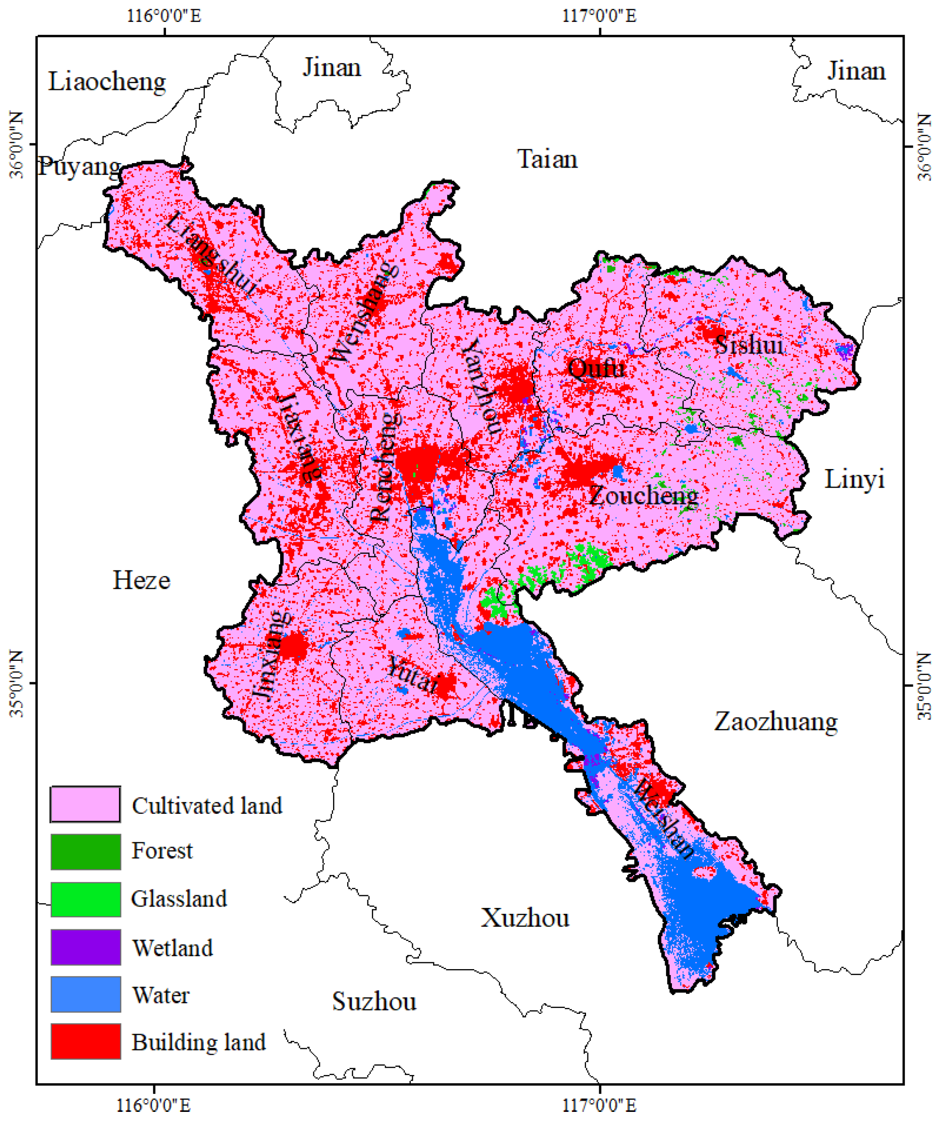
Based on the entropy weighting method, we determined the weights of the IRSEI index to improve the stability of the model. This was a case study to illustrate the advantages of the improved method. Through the geographically weighted regression (GWR) model, the relationship between urban ecological environment quality and human activity factors was visualized. The study included three main steps: (1) using remote sensing images to obtain the single remote sensing ecological indices from 2000 to 2020; (2) comparing the IRSEI model and RSEI model to evaluate spatiotemporal changes for three periods in the study area, and then merging the annual remote sensing ecological index; and (3) using GWR to explore the relationship between the IRSEI and human activity factors. The flow chart for the details is given in Figure 1.

2.1. Study Area

Jining (34°26′–35°57′ N, 115°52′–117°36′ E), located in the southwestern part of Shandong Province, is one of the central cities in the important Huaihai Economic Zone in China (Figure 2). Its terrain is dominated by plains and depressions, with high terrain in the east and low terrain in the west. The plain area of the city is mainly occupied by agricultural and construction land. Forests and grasslands are concentrated in the mountainous hills to the east, and Nansi Lake, the largest lake in Shandong Province, is located to the southeast. As an important transportation hub city, Jining covers 11 districts including Rencheng District, Yanzhou District, Zoucheng City, Qufu City, Weishan County, Yutai County, Jinxiang County, Jiaxiang County, Wenshang County, Sishui County and Liangshan County. In 2022, Jining achieved a regional GDP of RMB 531.69 billion, with a year-on-year growth of 4.4%.

2.2. Data Sources and Preprocessing

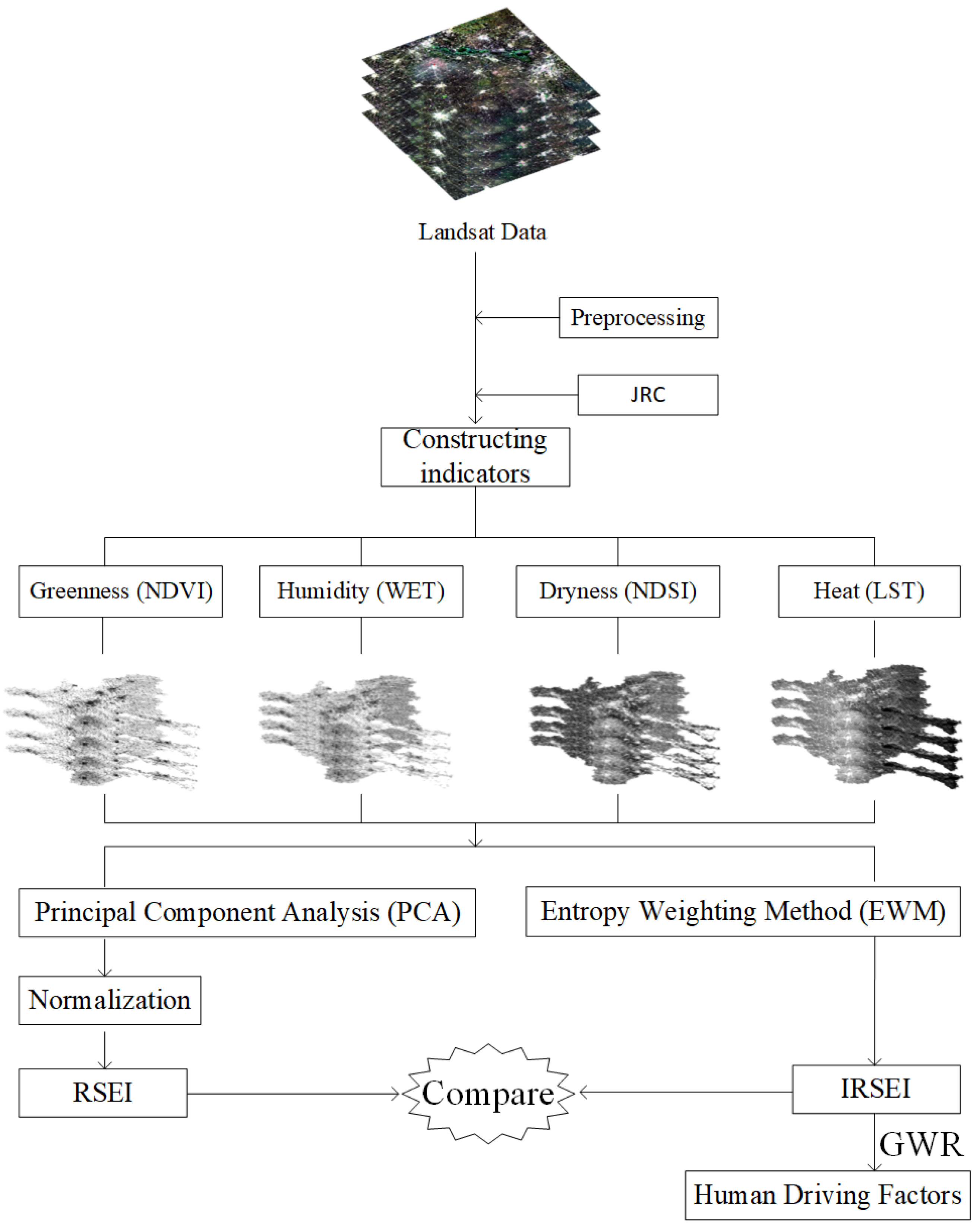
Eight Landsat5 TM and four Landsat8 OLI images were used to generate the model index for three periods in 2000, 2010 and 2020. According to the Jining seasonal division, December to February is winter, March to May is spring, June to August is summer and September to November is autumn [18,19]. All images were selected to match Jining’s seasonal division, but due to constraints in data acquisition, missing images were replaced with data from adjacent years. Gross domestic product (GDP), population density, nighttime lighting data and road network data were selected for analysis of urban factors affecting environmental quality. To maintain consistency with the spatial resolution, the above data were resampled to 30 m. In addition, the paper masked the water bodies to avoid affecting the model evaluation results, as the remote sensing ecological index model is not suitable for water body objects. We used the JRC Global Surface Water Mapping Layers to extract and mask the water bodies including seasonal and perennial water bodies in the study area. Further details are given in

Table 1. Data sources.

Data Type	Resolution	Processing and Methodogy		Source
2000–2020 remote sensing images	30 m	Geometric correction	Nearest	USGS (https://www.usgs.gov/) (accessed on 2 March 2022)
		Mosaicking	Nearest Neighbor
		Cropping	-
JRC Global Surface Water Mapping Layers	30 m	Cropping	-	JRC JEODPP Data Browser (https://jeodpp.jrc.ec.europa.eu/) (accessed on 5 May 2022)
		Vectorization	-
GDP (2000\2010\2019)	1 km	Formula calculation	-	Resource and Environment Science Data Center (http://www.resdc.cn/) (accessed on 12 July 2022)
		Cropping	-
		Resampling	-
Population density	100 m	Cropping	-	WorldPop (https://hub.worldpop.org/) (accessed on 13 July 2022)
		Resampling	Bilinear
Nighttime lighting data (2000\2010\2020)	1 km	Cropping	-	National Tibetan Plateau Data Center (http://data.tpdc.ac.cn) (accessed on 15 July 2022)
		Resampling	Bilinear
Road network data (2020)	30 m	Formula calculation	-	OpenStreetMap (https://www.openstreetmap.org/) (accessed on 26 August 2022)
		Cropping	-
		Resampling	Bilinear

.

2.3. Methodology

2.3.1. Constructing the IRSEI and RSEI

The four ecological indicators of greenness, humidity, heat and dryness are closely linked to ecological environment quality, so vegetation index, wetness component and surface temperature can be used to represent greenness, humidity and heat, respectively. Furthermore, the impervious surfaces of buildings and bare soil are related to urban dryness. The building and bare soil indices can be used to represent dryness. The formulas for the four ecological indices are shown in

Table 2. Formulas and references of the four ecological indicators.

Indicators	Calculation Formula	Explanation
Greenness	$NDVI=\left({\rho }_{NIR}-{\rho }_{Red}\right)/\left({\rho }_{NIR}+{\rho }_{Red}\right)$	${\rho }_{NIR} \mathrm{and} {\rho }_{Red}$ for the near-infrared band and the red band, respectively [7].
Humidity	$\begin{array}{cc}\hfill {\mathrm{WET}}_{TM}=& 0.0315{\rho }_{Blue}+0.2021{\rho }_{Green}+0.3102{\rho }_{Red}\hfill \\ \hfill & +0.1594{\rho }_{NIR}-0.6806{\rho }_{SWIR1}-0.6109{\rho }_{SWIR2}\end{array}$ $\begin{array}{cc}\hfill {\mathrm{WET}}_{OLI}=& 0.1511{\rho }_{Blue}+0.1972{\rho }_{Green}+0.3283{\rho }_{Red}\hfill \\ \hfill & +0.3407{\rho }_{NIR}-0.7117{\rho }_{SWIR1}-0.4559{\rho }_{SWIR2}\end{array}$	${\rho }_{Blue}, {\rho }_{Green}, {\rho }_{Red}, {\rho }_{NIR}, {\rho }_{SWIR1}\mathrm{and} {\rho }_{SWIR2}$ correspond to the reflectance of TM and OLI remote sensing images, respectively [7,12].
Heat	$LST=\frac{\mathrm{T}}{\left[1+\left(\frac{\mathsf{\lambda }\mathrm{T}}{\mathsf{\rho }}\right)\times \ln \mathsf{\epsilon }\right]}-273.15$	Calculated with reference to [20].
Dryness	$NDSI=\frac{IBI+SI}{2}$ $\begin{array}{cc}\hfill IBI=& \{\frac{2{\rho }_{SWIR1}}{{\rho }_{SWIR1}+{\rho }_{NIR}}-[\frac{{\rho }_{NIR}}{{\rho }_{NIR}+{\rho }_{Red}}+\frac{{\rho }_{Green}}{{\rho }_{Green}+{\rho }_{SWIR1}}\left]\right\}/\{\frac{2{\rho }_{SWIR1}}{{\rho }_{SWIR1}+{\rho }_{NIR}}+\hfill \\ \hfill & [\frac{{\rho }_{NIR}}{{\rho }_{NIR}+{\rho }_{Red}}+\frac{{\rho }_{Green}}{{\rho }_{Green}+{\rho }_{SWIR1}}]\}\hfill \end{array}$ $\begin{array}{cc}\hfill SI=& \left[\left( {\rho }_{SWIR1}+{\rho }_{Red}\right)-\left( {\rho }_{NIR}+{\rho }_{Blue}\right)\right]\hfill \\ \hfill & /\left[\left( {\rho }_{SWIR1}+{\rho }_{Red}\right)+\left( {\rho }_{NIR}+{\rho }_{Blue}\right)\right]\hfill \end{array}$	SI represents soil index, IBI represents building index other bands are interpreted as above [7].

.

Principal component analysis (PCA) is the main method of RSEI [21]. Unlike RSEI, the entropy weighting method (EWM) is applied to determine the weights of each remote sensing ecological index and then construct the new model. Considering the seasonal variability, this paper synthesized the annual IRSEI and RSEI after analyzing the seasonal changes as follows:

$$RSEI=f_{PCA}\left(NDVI, WET, NDSI, LST\right)$$

(1)

$$IRSEI=f_{EWM}\left(NDVI, WET,NDSI, LST\right)$$

(2)

where NDVI represents greenness, WET represents wetness, normalized soil index (NDSI) represents dryness and LST represents heat. To reduce the impact of water on RSEI and IRSEI models, each indicator needed to be water masked. To avoid the effect of indicator scale differences on weights, standardization of each indicator was necessary before applying PCA or EWM. NDVI and WET were positively normalized using Formula (3), while NDSI and LST were negatively normalized using Formula (4). The formulas are as follows:

$$Y=\frac{x-x_{min}}{x_{max}-x_{min}}$$

(3)

$$Y=\frac{x_{max}-x}{x_{max}-x_{min}}$$

(4)

where $Y$ is the normalized index values, $x$ is the value of the index in a certain pixel, $x_{min}$ is the minimum value of the index and $x_{max}$ is the maximum value of the index.

(1)

RSEI model

In the RSEI model, the first principal component (PCA1) after using principal component analysis (PCA) was used to calculate the RSEI, which could explain more than 90% of the total variation in the dataset. To make the value of PCA1 positively correlate with the ecological environmental quality, the $RSE{I}_0$ was expressed using Formula (5). Then $RSE{I}_0$ was normalized to denote sensible results.

$$RSE{I}_0=1-PCA1\left[F\left(NDVI,WET,NDSI,LST\right)\right]$$

(5)

$$RSEI=\left( RSE{I}_0-RSE{I}_{0MIN}\right)/\left( RSE{I}_{0MAX}-RSE{I}_{0MIN}\right)$$

(6)

where $PCA1$ is the first principal component of the four indicators.

(2)

IRSEI model

The same indicator images, 12 images in total for three periods, were superimposed. After sampling the raster values, the data values were calculated using the entropy method to obtain the entropy weights corresponding to the different indicators of IRSEI with Python. The calculation steps are shown below.

First, calculate the weighting of the indicators:

$$P_{ij}=X_{ij}/\left({\displaystyle \sum }_{i=1}^m{X}_{ij}\right)$$

(7)

where $P_{ij}$ is the weight of the $i$th valid data rows in $j$th indicator; $X_{ij}$ is the $i$th valid data rows in $j$th indicator; $j=1, 2, 3, 4$, for NDVI, WET, NDSI and LST, respectively; and $m=13027375$

Second, define entropy:

$$e_j=-\frac{1}{\ln m}{\displaystyle \sum }_{i=1}^m{P}_{ij}ln{P}_{ij}$$

(8)

where $e_j$ is the entropy value of the $j$th indicator, $m=13027375$ and $ln$ is the natural logarithm.

Third, determine the entropy weights.

$$w_j=\left(1-e_j\right)/{\displaystyle \sum }_{j=1}^n(1-e_j)$$

(9)

where $w_j$ is the entropy weight of the $j$th indicator, $n=4$ and $w_j$ is between 0 and 1 and satisfies ${\displaystyle \sum }_{j=1}^n{w}_j=1$.

Finally, linear weighting was performed. Based on the results of the entropy method, the seasonal IRSEI was calculated in ENVI as follows:

$$IRSEI={\displaystyle \sum }_{j=1}^n{w}_j\times x_j$$

(10)

where $x_j$ is the remote sensing image after normalization of the $j$th indicator.

The value of RSEI or IRSEI ranges between [0,1], and values closer to 1 indicate better ecological environment quality. According to the evaluation system of Xu and other scholars, they were divided into five levels: poor (0–0.2), fair (0.2–0.4), moderate (0.4–0.6), good (0.6–0.8) and excellent (0.8–1.0) [7,11,15].

2.3.2. Geographically Weighted Regression

Geographically weighted regression (GWR) is a local linear regression model that highlights the spatial heterogeneity of variables by combining spatial correlation with linear regression to improve on traditional models [22,23]. Ordinary least squares (OLS) is the simplest of the regression analysis methods, but the results do not reflect local variations in space [24]. In contrast, GWR can better reveal the distribution relationships among geographical variables in geographical locations, reflecting the local characteristics of geographical variables. Therefore, this paper adopted the GWR model for further analysis and research. Its equation is as follows:

$$Y_i={\beta }_0\left(u_i,v_i\right)+{\displaystyle \sum }_k{\beta }_k\left(u_i,v_i\right)X_{ik}+{\epsilon }_i$$

(11)

where $Y_i$ denotes the dependent variable, $\left(u_i,v_i\right)$ denotes the geographic coordinates of the $i$th point, ${\beta }_0\left(u_i,v_i\right)$ denotes the intercept of the $i$ th point, ${\beta }_k\left(u_i,v_i\right)$ denotes the coefficient of $X_{ik}$ and ${\epsilon }_i$ denotes the residual of the $i$ th point.

3. Results

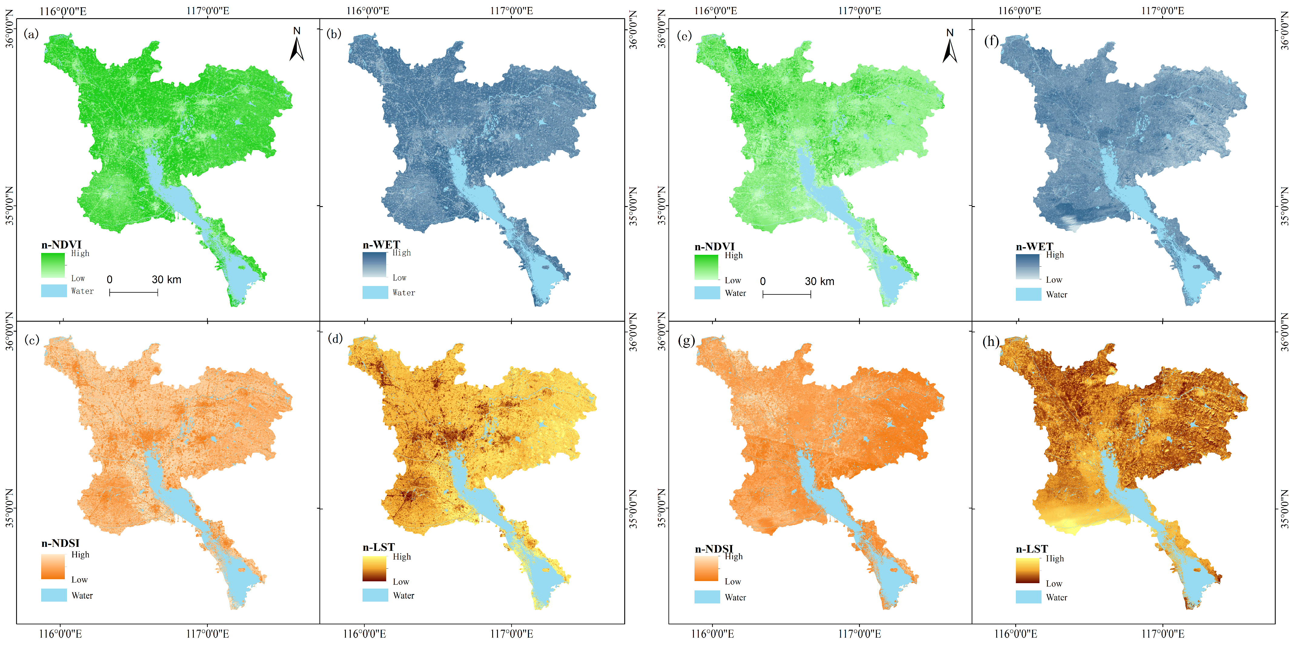
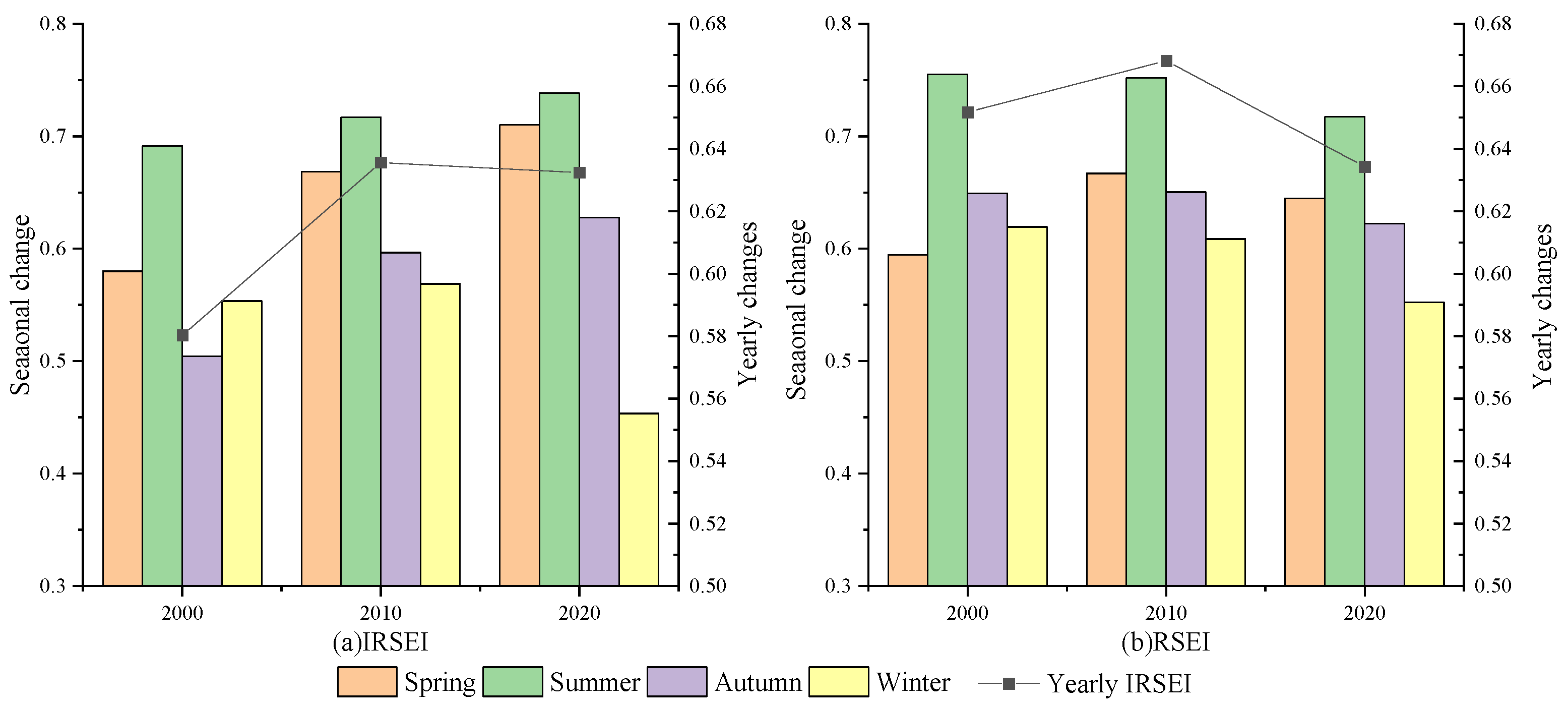
3.1. Changes in the Indices

Before applying the models, it was necessary to analyze the indices in this study. Figure 3 shows the mean values of the four indices in the different seasons of the different years over the whole area. The seasonal variation in NDVI, WET and LST featured an increase followed by a decrease, while the change in NDSI showed the opposite trend. Furthermore, it was clear that the highest NDVI and WET values, but the lowest NDSI value, occurred in summer. The highest LST values were mainly concentrated in the summer months, except in 2010. The LST in summer 2020 was significantly higher than in other years. The above analysis refers to Jining’s warm temperate monsoon climate, which is hot and rainy in summer, but sunny and cold in winter.

In conjunction with previous studies, the greenness (NDVI) and wetness (WET) indicators had a positive effect on ecological environmental quality, while the dryness (NDSI) and heat (LST) indicators had a negative effect on ecological environmental quality [7,25,26]. For more visual analysis of the spatial distribution of the indices, the individual indices were normalized and visualized for summer and winter in 2020 (Figure 4). Note that the color directions representing the normalized NDVI and WET minimum and maximum are different from those of the normalized NDSI and LST. On the normalized NDVI maps, the n-NDVI values around the central urban area were relatively high whatever the period, which could be caused by a reduced vegetation cover in this area. At the same time, the whole study area was greener in summer than in December, as hot and rainy days are more conducive to vegetation growth. Furthermore, the spatial distribution of n-WET was similar to that of n-NDVI. Compared to the n-NDSI and n-LST in summer, it is interesting to note that their distribution was the same, whereas in winter it was not clear.

3.2. Comparative Analysis of IRSEI and RSEI

The entropy weighting method was used to integrate the indices. In this paper, the annual IRSEI values in the study area were calculated. The entropy weights in

Table 3. Entropy weights of NDVI, WET, NDSI and LST.

	NDVI	WET	NDSI	LST
Entropy weight/%	54.60	5.60	15.57	24.26

revealed the role of each indicator in influencing the ecosystem. It could be seen that in descending order of entropy weight the NDVI, LST, NDSI, WET, NDVI and LST had greater weights, which was closely related to the climate, and NDVI may be related to the large area of cultivated land in the study area and the tillage system of growing two crops per year. We could obtain the characteristics of seasonal changes in ecological quality in the study area using the IRSEI model (Figure 5a). The ecological quality improved in spring, summer and autumn, and increased but then decreased in winter. The RSEI model obtained using principal component analysis (Figure 5b) showed that there were seasonal differences in ecological quality. In spring and autumn, the RSEI rose and then fell; in other seasons, it showed a decreasing trend. Based on the seasonal differences in the remotely sensed ecological environment quality, the annual IRSEI or RSEI had to be calculated to represent the combined index. Using the averages of annual IRSEI and RSEI, we found that both the IRSEI and RSEI showed an ascending then descending trend from 2000 to 2020, but the IRSEI showed that the overall ecological environmental quality level was improving in the study area.

It is worth noting that RSEI results must be artificially evaluated for their indication results. This is because if there is an area with a high ecological index, indicating a poor ecological environment, it must be inverted to obtain the correct image of the remote sensing ecological index. The entropy weighting method can avoid this problem through determining the weights and then obtaining the correct remote sensing ecological index directly, which is easier to apply.

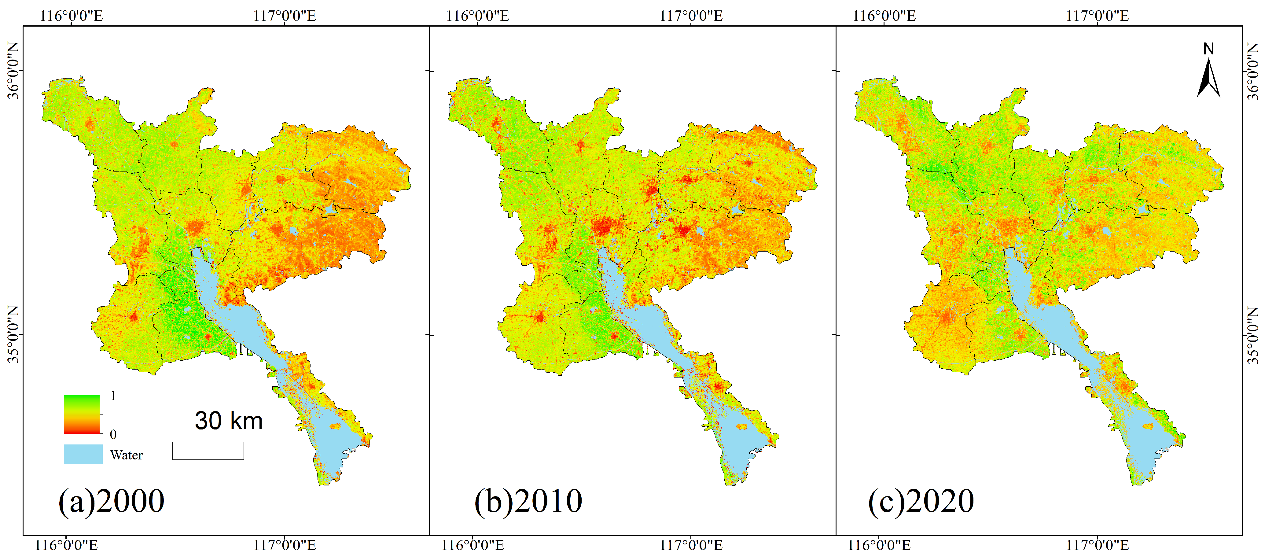
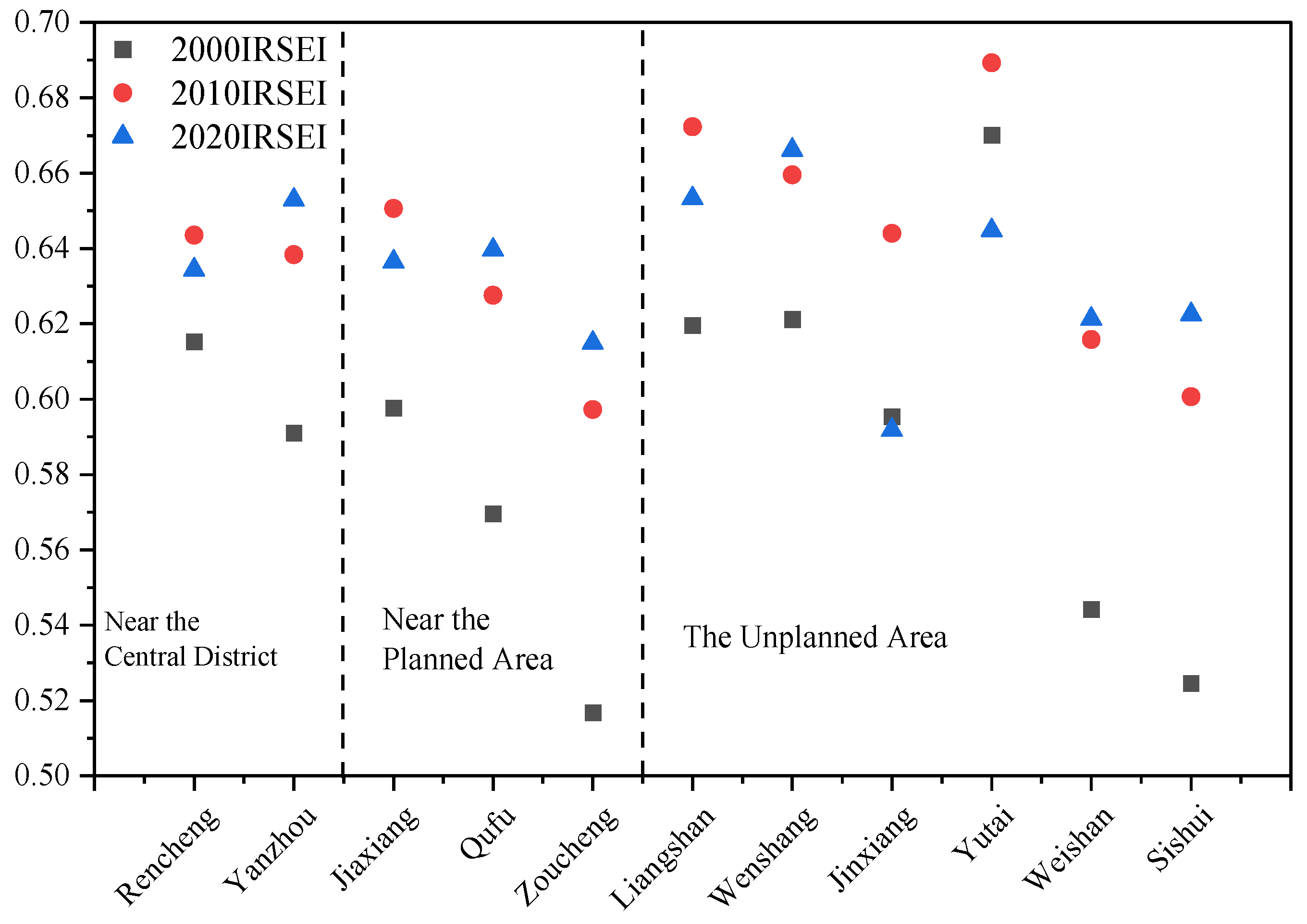
3.3. Spatiotempral Distribution of IRSEI

To further analyze the differences in spatial distribution, the IRSEI results were divided into five grades of poor, fair, moderate, good and excellent at an interval of 0.2. Figure 6 shows the distribution of ecological classes in Jining City. Overall, most of Jining was at moderate and good IRSEI levels, with only small parts at the poor, fair and excellent levels. The central urban area of the county remained at the moderate level during the 20 years. The eastern mountainous region was also at the moderate level. In terms of the spatial distribution of IRSEI scores, the ecological quality of the southwestern part of Jining was generally better than that of the northeastern part. The ecological quality of the urban area in each county improved, while the external ecological quality around the adjacent urban area declined. This was closely related to urbanization and the expansion of the built-up area. Areas of good and excellent ecological environment quality classes were mainly distributed in the western plain regions, which showed an irregular distribution.

In summary, the IRSEI model revealed the ecological environment quality of the different areas, which met the need to reflect the spatial distribution of ecological environmental quality. The IRSEI was reasonable as an indicator of urban ecological environmental quality.

The change detection statistics for IRSEI showed that all RSEI levels were transformed into each other (

Table 4. Area of IRSEI grade change.

Grade Change	2000–2010		2010–2020		2000–2020
	Area (km2)	Percentage	Area (km2)	Percentage	Area (km2)	Percentage
Better	3074.21	30.90%	793.67	7.99%	2980.93	30.12%
Unchanged	6657.92	66.91%	7733.95	77.88%	6147.59	62.12%
Worse	218.11	2.19%	1402.58	14.12%	767.39	7.75%
Total	9950.24	100.00%	9930.20	100.00%	9895.91	100.00%

). The water bodies at different times were different, so this study considered the partial conversion of water into non-water as an improvement in environmental quality and the conversion of non-water into water as a deterioration in environmental quality.

During the period from 2000 to 2010, the area converted to a worse ecological environment quality was 218.11 km² and the area converted to a better ecological environment quality was 3074.21 km², accounting for 2.19% and 30.90% of the effective study area in Jining, respectively. The area transferred to poor and fair quality was 30.51 km² and the area transferred to good and excellent quality was 2989.59 km². From 2010 to 2020, the area converted to a worse ecological environment quality was 1402.58 km², accounting for 14.12% of the area, and the area converted to a better ecological environment quality was 793.67 km², accounting for 7.99%. The area transferred to poor and fair quality was almost unchanged, while the area transferred to good and excellent quality was 770.62 km². In general, the total ecological quality was improving. There was a more obvious recovery of ecological environment quality, mainly reflected in a large number of areas with fair and poor ecological environment quality reaching moderate quality during 2000–2020. Furthermore, some water bodies have undergone land-type conversion, which increased the effective assessment area of the ecological quality in the study area.

In order to better assess the environmental quality of Jining City, the IRSEI changes at the county levels are shown in Figure 7. In accordance with the Jining City Urban Master Plan (2014–2030), the eleven districts were divided into three areas, namely, the near-central urban area, the near-planning area, and the non-planning area. Over the past 20 years, the ecological index of Rencheng District, which is near the central urban area, has risen and then fallen, but the overall ecological quality has improved; the ecological environment in Yanzhou District has gradually improved. The ecological improvement in the three areas close to the planning area was more obvious, but the IRSEI in Jiaxiang County rose and then fell, showing an overall upward trend. There were significant differences in the changes in IRSEI in the counties in the non-planning areas. For example, the ecological quality in Wenshang, Weishan and Sishui counties improved year by year, while the IRSEI in Liangshan, Jinxiang and Yutai counties first increased and then decreased. Based on previous land use data for Jining, except for the mountainous distribution areas of Zoucheng County, Sishui County and Jiaxiang County, the areas with low ecological environment quality index values in each county basically coincided with the expansion areas of building land in the corresponding period. This showed that the decrease of ecological environment quality in urban areas was related to the construction of urban houses and surrounding roads in the study area.

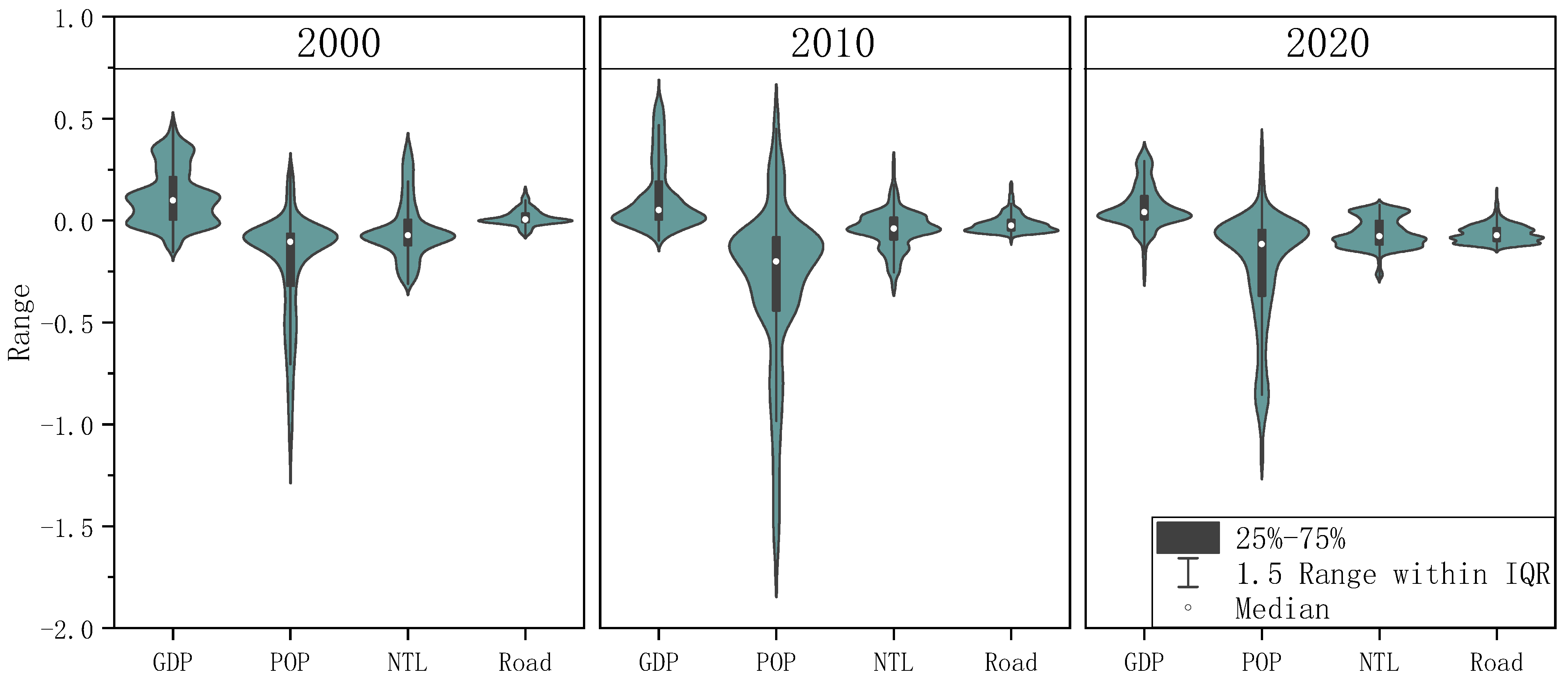
3.4. Analysis of Ecological Environmental Quality Driver

3.4.1. Global Spatial Autocorrelations

In order to reduce the influence of the varying scales in GWR on the spatial characteristics, varying scales were used in the study [23]. This paper explored the spatial correlation of IRSEI in the study area from 2000 to 2020 using the fishing net of four scales (1500 m × 1500 m, 2000 m × 2000 m, 2500 m × 2500 m and 3000 m × 3000 m) in ArcGIS.

Table 5. IRSEI Moran’s index at different scales.

	2000			2010			2020
	Moran’s I	z	p	Moran’s I	z	p	Moran’s I	z	p
1500 m	0.573	94.653	0.000	0.542	89.591	0.000	0.567	78.566	0.000
2000 m	0.630	47.733	0.000	0.607	46.113	0.000	0.608	46.041	0.000
2500 m	0.625	38.189	0.000	0.602	36.794	0.000	0.607	37.051	0.000
3000 m	0.609	31.247	0.000	0.585	30.012	0.000	0.588	30.132	0.000

demonstrated that the confidence levels at all four scales were higher than 99%, indicating that the spatial autocorrelation of IRSEI for 2000–2020 was quite strong. On the same scale, Moran’s I showed a decreasing trend from 2000 to 2010 and a gradually increasing trend from 2010 to 2020. Overall, Moran’s I was higher in the year 2000 than in the year 2020, suggesting a slight increase in the spatial aggregation effect of IRSEI in Jining. With an increasing scale, Moran’s I increased and then decreased in 2000 and 2010, and the z values started to decrease in all three periods, indicating that as the sampled grid increased, the homogenization between grids increased, and when the grid became too large, the information within the grid may have been lost and the IRSEI may no longer be spatially autocorrelated.

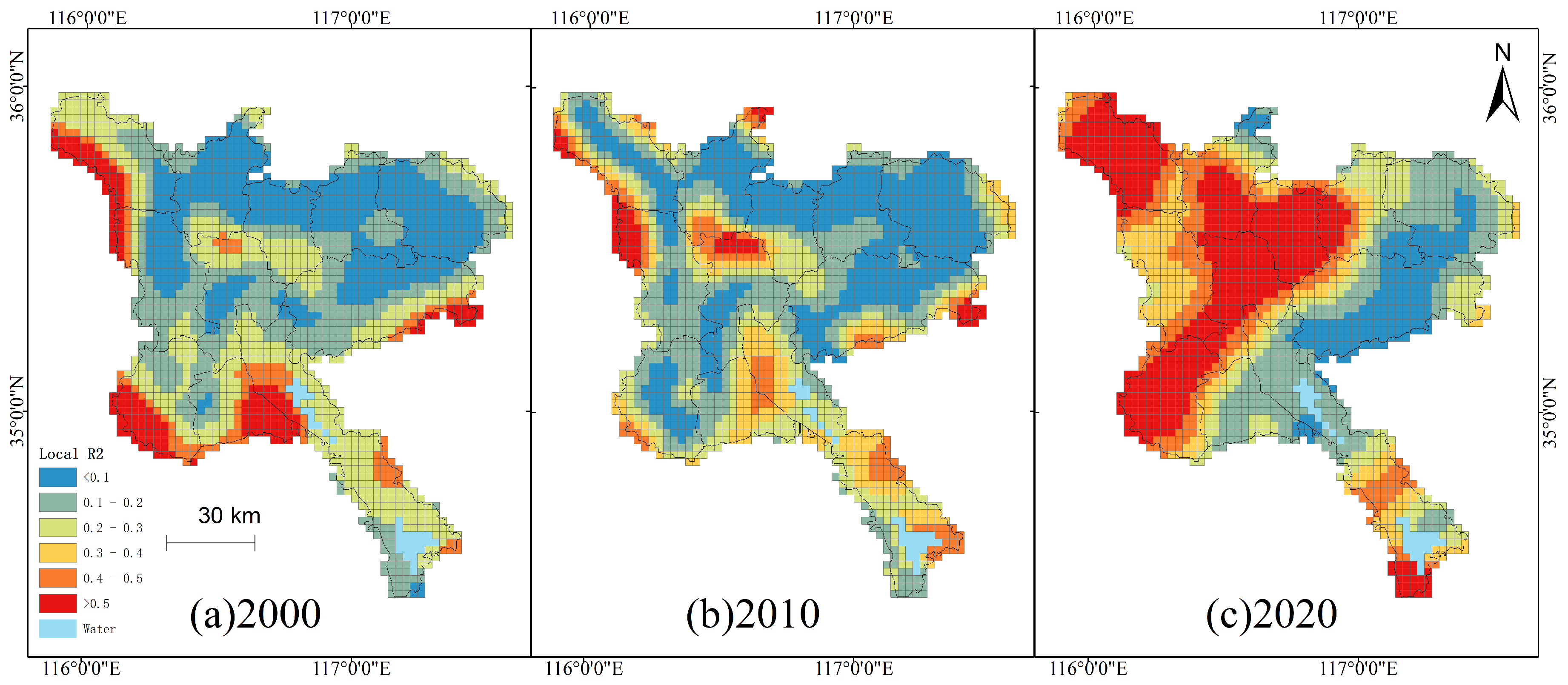
3.4.2. Results of GWR-Based Regression Coefficients of Driving Factors

According to the results presented in Section 3.3, the distribution of IRSEI in Jining City was uneven. Further research on the spatial influence of factors on IRSEI is needed. Therefore, the local regression coefficients in GWR were used to analyze the spatial and temporal differences in human activity factors and their direction and intensity. In this study, we chose the nighttime light index (NTL), population density (POP), road density (Road) and economic level as the main human driving factors that are representative.

Table 6. Comparison of GWR and OLS.

Model	Scale/km2	2000			2010			2020
		AICc	R2	R2 Adjusted	AICc	R2	R2 Adjusted	AICc	R2	R2 Adjusted
Geo-weighted regression (GWR)	1.52	−8064.885	0.636	0.619	−7124.161	0.611	0.590	−5102.653	0.391	0.381
	22	−3128.020	0.430	0.420	−2914.127	0.465	0.450	−2571.443	0.387	0.374
	2.52	−2939.980	0.695	0.664	−2595.370	0.688	0.649	−2216.013	0.598	0.562
	32	−1914.689	0.684	0.645	−1724.518	0.702	0.649	−1425.883	0.589	0.544
Least squares regression (OLS)	1.52	−3453.493	0.056	0.055	−2753.340	0.030	0.029	−2843.504	0.038	0.038
	22	−1727.017	0.071	0.070	−1271.876	0.041	0.040	−1332.177	0.049	0.048
	2.52	−1074.246	0.095	0.093	−753.246	0.059	0.057	−796.346	0.068	0.066
	32	−691.520	0.101	0.098	−465.933	0.066	0.064	−498.346	0.072	0.069

showed that the GWR fitted the human activity factors and IRSEI much better than the ordinary least squares (OLS) model. At the same time, the R² results for GWR were mostly greater than 0.5, much higher than for OLS, and the difference between the Akaike Information Criterion (AICc) was much greater than 3. The difference was clear, indicating that GWR was more suitable than OLS for indicators of environmental quality and human activity in the study area.

The regression coefficients of GWR were spatially displayed using ArcGIS at the scale of 2500 m × 2500 m to reflect the relationship between ecological environment quality and human activity factors in Jining City, and the spatial distribution is shown in Figure 8. The local R² can explain the degree and extent of the impact of human activity on the ecological environment quality. The impact of human activity factors on the ecological environment in Jining during the same period showed a strong impact in the northwest and a weak impact in the southeast. There was a spatial divergence between the ecological environment index and human activities. Over time, the explanatory power of human activities on the ecological environment quality of the whole study area increased and the explanatory range expanded, except for in the eastern mountainous areas and the areas near Dushan Lake and Zhaoyang Lake.

Table 7. Results of GWR operations.

	Driving Factor	Minimum	Median	Maximum	Average	Percentage of Positive	Percentage of Negative
2000	GDP	−1.807	0.480	16.824	1.873	82.45%	17.55%
	POP	−11.506	−0.568	7.721	1.530	18.56%	81.44%
	NTL	−0.207	−0.083	2.365	0.492	37.93%	62.07%
	Road	−0.761	0.150	3.225	0.321	78.90%	21.10%
2010	GDP	−11.581	0.191	18.657	1.667	69.16%	20.84%
	POP	−15.002	−0.328	10.985	1.391	27.44%	72.56%
	NTL	−7.075	−0.071	2.878	0.535	36.51%	63.49%
	Road	−1.084	0.113	3.418	0.379	70.53%	29.47%
2020	GDP	0.912	0.028	0.807	0.161	63.73%	36.27%
	POP	−1.295	−0.144	3.717	0.320	18.81%	81.19%
	NTL	−0.328	−0.061	0.274	0.086	25.86%	74.14%
	Road	−0.273	−0.066	0.420	0.079	18.86%	81.14%

shows the minimum, maximum, median and mean of the absolute values, the proportion of positive values and the proportion of negative values of GWR to analyze the relevance and direction of the impact of human-driven factors on the ecological environment index. In combination with Figure 9, the regression coefficients showed that all four human activity factors had positive and negative correlations with the IRSEI in the study area. In terms of the average of the absolute values at the regression coefficients, the correlations of human activity factors over the same period were, in descending order, GDP, POP, NTL and Road in 2000 and 2010. In 2020, it was POP, GDP, NTL and Road. Over time, the average correlation effect of GDP, POP and Road decreased over time, and NTL grew but then declined. In terms of the percentage of regression coefficients, GDP had a positive correlation with the improvement of the quality of the ecological environment. The Road factor only had a negative correlation in 2020, while POP and NTL negatively correlated with the improvement of the ecological environment.

4. Discussion

4.1. Calculation of IRSEI

In this paper, the entropy weighting method performed better for the same type of data with significant differences. The vegetation growth in Jining was good in summer, and the greenness index did not change much over the three study periods, so the index weight was smaller in summer. Although the remote sensing data for different periods in summer and autumn cover a small timespan of about one month due to the limitations of cloud cover and time of acquisition, the average values of the greenness index showed that vegetation growth in summer was significantly better than in the adjacent spring and autumn seasons. In addition, as in previous studies, the vegetation index and drought index had a greater influence on the quality of the ecosystem. Furthermore, Jining is home to the largest freshwater lake in Shandong Province, and the lake wetland ecosystem is typically representative of the area. In this study, seasonal and permanent water bodies were masked to reduce the contribution of water bodies to the calculation of the city’s remote sensing ecological index. The ecological impact of water will be further integrated into the ecological environmental quality assessment of Jining City in the future.

4.2. Driving Forces of Ecological Environment Quality

In conjunction with relevant literature, the causes of regional differences in ecological environment quality in the study area are discussed here. First, the urban spatial structure was inappropriate. The conflict between people and land is becoming more pronounced. Regional differences in urbanization in Jining are obvious. The population showed uneven characteristics in spatial distribution, with population density higher than the average in Shandong Province, but the level of urban construction low, and the development of the urban system was going backwards [27]. At the same time, land use was inappropriate, with a large amount of arable land, grassland and forest being converted to construction land [28]. From the literature [29,30], it can be seen that the area of forest land in Jining showed a trend of first increasing and then decreasing from 2000 to 2015, and the area of grassland decreased, while the area of urban housing showed a continuous increase. In addition, the accelerated urbanization process cannot be separated from the development and construction of the transport road network [28]. The various forms of damage and pollution caused by the construction and use of roads inevitably have a negative impact on the regional ecological environment. From monitoring the changes in the ecological environment in the study area, it can be intuitively seen that the traffic road network was radially distributed, with town houses at the center, and the ecological environment quality in and around the road network showing a decline. Second, as a central city in the important Huaihai Economic Zone, Jining is also one of China’s coal-based mature cities. According to the Jining City Urban Master Plan (2014–2030), its coal resources were known to be concentrated in the central city and the planning area, with Weishan County, Wenshang County, Jinxiang County and Yutai County in the non-planning area. While large-scale coal mining brought economic benefits, it also caused significant environmental problems at the cost of local ecological damage [31], such as landscape fragmentation [32], soil erosion, vegetation degradation, biodiversity loss and the collapse of coal mining areas [33]. Finally, the management of rural environmental pollution remained a major challenge in the context of rural revitalization strategies. Many practices are not conducive to promoting the improvement of the regional ecology such as imperfect pollution management mechanisms, untimely management information, insufficient applicability of management facilities and a low level of environmental awareness among enterprises and the public [34]. In summary, the impact of human activities on the ecological environment in the study area is obvious.

Based on the above analysis, this paper analyzed the spatial heterogeneity of remote sensing ecological indices and human driving factors through a geographically weighted regression model. Human activity is a complex process [35]. In this paper, the economic level, population density, nighttime lighting data and road network density were used to represent the intensity of human activities in an integrated manner. The results showed that the intensity of human activity has both positive and negative effects on regional environmental stress. Among them, GDP showed a greater role in promoting ecological environment quality improvements than inhibiting it in GWR models. According to the Jining Statistical Yearbook 2020, its GDP per capita increased from 7032 yuan in 2000 to 27,750 yuan in 2010 and reached 53,773 yuan in 2020, showing an obvious upward trend. From the industrial structure, the ratio of the three industrial structures in Jining was 21:43.4:35.6 in 2000, 13.5:51.4:35.1 in 2010 and 11.7:39.2:49.1 in 2020. In Jining, the share of primary industry fell, the share of secondary industry rose and then fell and the share of tertiary industry fell and then rose. The industrial structure of the study area has undergone an obvious adjustment. In addition, the main industry in each district was replaced with electronic information, new materials, high-end equipment, etc. The high-tech industry output value above the proportion of industry is slowly increasing year by year. Research and development investment funds are increasing too. Investment in research and development is conducive to promoting technological progress and the development of new energy, thus, reducing the emissions of pollutants, which may alleviate environmental pressure [36]. Therefore, high-quality economic development may play a positive role in improving the ecological environment in Jining, and in the future development process, we should continue to improve the investment in research and development, promote industrial upgrades and avoid the high pollution levels brought by the one-sided pursuit of profits. At the same time, attention should be paid to the destructive effects of coal mining, with timely environmental restoration and protection of existing forest resources. The results of the analysis of population density and nighttime lighting data showed that dense population and human activities have a negative impact on the ecological environment. The urbanization rate in Jining was 23.8%, 43% and 60.1% in 2000, 2010 and 2020, respectively, which represents rapid urbanization. The government should moderately control the speed of population concentration, reasonably plan the land for housing and roads and pay attention to environmental protection by reducing population congestion. In conclusion, it is important to give full play to the role of government regulation and economic upgrading in order to coordinate the relationship between urban and economic development, reduce the pressure of urban development on the ecological environment and ease the ecological restoration work of future urbanization construction.

Due to the availability of road data, the road network density for the three periods was calculated based on the road network data in 2020 without considering the changes in the road construction process; meanwhile, future research should try to add more data of related factors into the analysis and carry out the analysis of changes in urban ecological environment quality from both natural and human factors.

5. Conclusions

The proposed remote sensing ecological index (RSEI) provides a new evaluation model for the assessment of urban ecological environment quality. However, the principal component analysis method used in RSEI is not a direct indicator for ecological environment quality and the calculation process is complex. In this paper, we proposed to use the entropy weighting method to improve the construction of the model. Considering the seasonal changes, an improved remote sensing ecological index (IRSEI) was constructed using the entropy weighting method to dynamically monitor the ecological environment quality in the study area. Then, with analyzing the spatial distribution characteristics of ecological quality, the spatial relationship between the IRSEI and human activities was quantified using a geographically weighted regression (GWR). The results showed that the IRSEI constructed using the entropy weighting method is reasonable for revealing the distribution of urban ecological environment quality. Between 2000 and 2020, the urban remote sensing ecological index of Jining City showed an increase and then a decrease, but the ecological quality in general showed an upward trend. The regional ecological environment quality remained the same, with slight local increases and decreases. The GWR proved that human activities had better explanatory power for the spatial and temporal evolution of the improved remote sensing ecological index, the explanatory power being stronger in the northwest than in the southeast in space, and the explanatory range expanding and the degree of explanatory power strengthening over time. Among them, the economic level showed a positive correlation with ecological environment quality, while population density and the night light index were mainly negatively correlated with ecological environment quality; the positive correlation of road network density on environmental quality varied over time. In future research, the IRSEI model based on the entropy weighting method can be used to directly reveal the regional state of ecology, so that the complexity of the workload is reduced.

References

1. Zhang, T.; Yang, R.; Yang, Y.; Li, L.; Chen, L. Assessing the Urban Eco-Environmental Quality by the Remote-Sensing Ecological Index: Application to Tianjin, North China. ISPRS Int. J. Geo-Inf. 2021, 10, 475. [Google Scholar] [CrossRef]
2. Zhang, H.; Yin, Y.; An, H.; Lei, J.; Li, M.; Song, J.; Han, W. Surface urban heat island and its relationship with land cover change in five urban agglomerations in China based on GEE. Environ. Sci. Pollut. Res. 2022, 29, 82271–82285. [Google Scholar] [CrossRef]
3. Yin, Y.; Zhang, H.; An, H.; Lei, J.; Li, M.; Song, J.; Han, W. Heat island characteristics and influencing factors of urban agglomerations in the Yangtze River Economic Zone based on gee. J. Ecol. 2023, 1, 1–13. [Google Scholar]
4. Zhuang, Q.; Wu, S.; Yan, Y.; Niu, Y.; Yang, F.; Xie, C. Monitoring Land Surface Thermal Environments under the Background of Landscape Patterns in Arid Regions: A Case Study in Aksu River Basin. Sci. Total Environ. 2020, 710. [Google Scholar] [CrossRef] [PubMed]
5. Jiang, L.; Liu, Y.; Wu, S.; Yang, C. Analyzing ecological environment change and associated driving factors in China based on NDVI time series data. Ecol. Indic. 2021, 129, 107933. [Google Scholar] [CrossRef]
6. Li, Y.; Cao, Z.; Long, H.; Liu, Y.; Li, W. Dynamic analysis of ecological environment combined with land cover and NDVI changes and implications for sustainable urban–rural development: The case of Mu Us Sandy Land, China. J. Clean. Prod. 2017, 142, 697–715. [Google Scholar] [CrossRef]
7. Xu, H.Q. A Remote Sensing Urban Ecological Index and Its Application. Acta Ecol. Sin. 2013, 33, 7853–7862. [Google Scholar]
8. Zhang, Y.; She, J.; Long, X.; Zhang, M. Spatio-temporal evolution and driving factors of eco-environmental quality based on RSEI in Chang-Zhu-Tan metropolitan circle, central China. Ecol. Indic. 2022, 144, 109436. [Google Scholar] [CrossRef]
9. Geng, J.; Yu, K.; Xie, Z.; Zhao, G.; Ai, J.; Yang, L.; Yang, H.; Liu, J. Analysis of Spatiotemporal Variation and Drivers of Ecological Quality in Fuzhou Based on Rsei. Remote Sens. 2022, 14, 4900. [Google Scholar] [CrossRef]
10. Gao, P.; Kasimu, A.; Zhao, Y.; Lin, B.; Chai, J.; Ruzi, T.; Zhao, H. Evaluation of the Temporal and Spatial Changes of Ecological Quality in the Hami Oasis Based on RSEI. Sustainability 2020, 12, 7716. [Google Scholar] [CrossRef]
11. Nong, L.; Wang, J. Dynamic monitoring of ecological environment quality in Kunming based on rsei model. J. Ecol. 2020, 39, 2042–2050. [Google Scholar]
12. Yang, W.; Zhou, Y.; Li, C. Assessment of Ecological Environment Quality in Rare Earth Mining Areas Based on Improved Rsei. Sustainability 2023, 15, 2964. [Google Scholar] [CrossRef]
13. Liu, Y.; Dang, C.-Y.; Yue, F.; Lv, C.-G.; Qian, J.-X.; Zhu, R. Comparative analysis of improved remote sensing ecological index and rsei. J. Remote Sens. 2022, 26, 683–697. [Google Scholar]
14. Hua, G.; Cen, H.; Shen, S.; Meng, Z.; Wu, J.; Shen, Z. Huaihai Blue Book: Huaihai Economic Zone Development Research Report (2020~2021); Social Sciences Academic Press: Beijing, China, 2021. [Google Scholar]
15. Pariha, H.; Zan, M.; Alimjia, K. Remote sensing evaluation of ecological environment in Urumqi city and analysis of driving factors. Arid. Zone Res. 2021, 38, 1484–1496. [Google Scholar]
16. An, M.; Xie, P.; He, W.; Wang, B.; Huang, J.; Khanal, R. Spatiotemporal change of ecologic environment quality and human interaction factors in three gorges ecologic economic corridor, based on RSEI. Ecol. Indic. 2022, 141, 109090. [Google Scholar] [CrossRef]
17. Xue, C.-L.; Zhang, H.-Q.; Zou, T.; Sun, Z.-J.; Cheng, H.-Y. Ecological quality of the Sino-Lao railroad economic corridor and its relationship with human activities. J. Appl. Ecol. 2021, 32, 638–648. [Google Scholar]
18. Cai, P.; Li, F.; Wang, Z.; Zhao, H. Correlation analysis of ground temperature and air temperature changes in Jining, Shandong Province, 1961–2015. Glacial Permafr. 2016, 38, 1538–1543. [Google Scholar]
19. Dong, X.-G.; Li, S.-L.; Shi, Z.-B.; Qiu, C. Change Characteristics of Agricultural Climate Resources in Recent 50 Years in Shandong Province, China. Ying Yong Sheng Tai Xue Bao = J. Appl. Ecol. 2015, 26, 269–277. [Google Scholar]
20. Alexander, C. Normalised difference spectral indices and urban land cover as indicators of land surface temperature (LST). Int. J. Appl. Earth Obs. Geoinf. 2019, 86, 102013. [Google Scholar] [CrossRef]
21. Xin, W.J.; Ma, J.M.; Wang, Y.Q. Ecological environment quality evaluation of Guilin city based on remote sensing ecological index. J. Guangxi Norm. Univ. (Nat. Sci. Ed.) 2022, 40, 1–14. [Google Scholar]
22. Fotheringham, A.S.; Brunsdon, C.; Charlton, M. Geographically Weighted Regression: The Analysis of Spatially Varying Relationships; John Wiley & Sons: Hoboken, NJ, USA, 2003. [Google Scholar]
23. Chen, X.; Zeng, X.; Zhao, C.; Qiu, R.; Zhang, L.; Hou, X.; Hu, X. Analysis of ecological effects of road networks based on remote sensing ecological indices—A case study of Fuzhou City. J. Ecol. 2021, 41, 4732–4745. [Google Scholar]
24. Xue, R.; Yu, X.; Li, D.; Ye, X. Exploring the influence of environmental heterogeneity on the spatial use of giant pandas in the Qinling Mountains based on a geographically weighted regression model. J. Ecol. 2020, 40, 2647–2654. [Google Scholar]
25. Shan, W.; Jin, X.; Ren, J.; Wang, Y.; Xu, Z.; Fan, Y.; Gu, Z.; Hong, C.; Lin, J.; Zhou, Y. Ecological environment quality assessment based on remote sensing data for land consolidation. J. Clean. Prod. 2019, 239, 118126. [Google Scholar] [CrossRef]
26. Shan, W.; Jin, X.; Meng, X.; Yang, X.; Xu, Z.; Gu, Z.; Zhou, Y. Dynamic monitoring of ecological and environmental quality of land remediation based on multi-source remote sensing data. J. Agric. Eng. 2019, 35, 234–242. [Google Scholar]
27. A Comparative Study on the Effect of Qi-Lu Cultural Differences on Regional Economic Development in Shandong. In Proceedings of the 2020 International Conference on Big Data Application & Economic Management (ICBDEM 2020), Guiyang, China, 27–28 March 2020.
28. Yao, Z.; Jiang, C.; Shan-Shan, F. Effects of urban growth boundaries on urban spatial structural and ecological functional optimization in the Jining Metropolitan Area, China. Land Use Policy 2022, 117, 106113. [Google Scholar] [CrossRef]
29. Yang, G.; Lu, N.; Xiao, X.; Ziegler, M. Analysis of Land Use in Jining City. E3S Web Conf. 2020, 198, 04024. [Google Scholar]
30. Wang, Y.; Zhao, Y.; Jiao, L.; Zou, Y. Changes in vegetation cover and influencing factors in Jining City from 2005–2016. J. Jinan Univ. (Nat. Sci. Ed.) 2018, 32, 171–177. [Google Scholar]
31. Krueger, H.; McLean, D.; Williams, D. Construction of Ecological Security Pattern Based on Ecological Sensitivity Assessment in Jining City, China. Prog. Exp. Tumor Res. 2008, 40, 1–6. [Google Scholar] [PubMed]
32. Guo, J.; Hu, Z.; Yuan, D.; Liang, Y.; Li, P.; Yang, K.; Fu, Y. Dynamic Evolution of Cultivated Land Fragmentation in Coal Mining Subsidence Area of the Lower Yellow River Basin: A Case Study of Jining City, Shandong Province. J. China Coal. Soc. 2021, 46, 3039–3055. [Google Scholar]
33. Shi, Y.; Guo, C.; Li, S.; Lu, F. Planning practice of ecological belt around Jining city. Planner 2018, 34, 52–58. [Google Scholar]
34. Weerasinghe, R.; Han, X.; Fang, C. Study on the Dilemma and Countermeasures of Rural Environmental Pollution Control under the Background of Rural Revitalization Strategy. E3S Web Conf. 2021, 237, 01030. [Google Scholar]
35. Zhang, S.-Y.; Fan, Y.-F.; Yan, L.; Xiao, X.-Z.; Li, H. A study on the spatial and temporal changes of ecological quality and its driving forces in Shaanxi Province in the past 20 years based on long time series modis. J. Soil Water Conserv. 2023, 37, 111–119+198. [Google Scholar]
36. Wang, S.; Gao, S.; Chen, J. A study of spatial heterogeneity of factors influencing haze pollution in Chinese cities based on the gwr model. Geogr. Stud. 2020, 39, 651–668. [Google Scholar]
Figure 1. Technical flow chart of the study.
Sustainability 15 08464 g001
Figure 2. Land use map of Jining in 2020.
Sustainability 15 08464 g002
Figure 3. Average in each season of each year for the study area.
Sustainability 15 08464 g003
Figure 4. Spatial distribution of the single remote sensing ecological indices in 2020. (a) the normalized NDVI in summer, (b) the normalized WET in summer, (c) the normalized NDSI in summer, (d) the normalized LST in summer, (e) the normalized NDVI in winter, (f) the normalized WET in winter, (g) the normalized NDSI in winter, (h) the normalized LST in winter.
Sustainability 15 08464 g004
Figure 5. Ecological quality changes based on IRSEI and RSEI.
Sustainability 15 08464 g005
Figure 6. The IRSEI level maps of (a) 2000, (b) 2010, (c) 2020.
Sustainability 15 08464 g006
Figure 7. IRSEI change in each county or district from 2000 to 2020.
Sustainability 15 08464 g007
Figure 8. Local R2 spatial distribution based on GWR (2500 m × 2500 m).
Sustainability 15 08464 g008
Figure 9. Statistics on the impact of human activities on IRSEI based on GWR.
Sustainability 15 08464 g009