


Parameter Extraction of Solar Photovoltaic Modules Using a Novel Bio-Inspired Swarm Intelligence Optimisation Algorithm

 ,
,  and
and 
Abstract
1. Introduction
- In order to estimate the parameters of the PV modules, this work seeks to propose the novel bio-inspired swarm intelligence OA called the DOA for the first time.
- SD and DD approaches are used to mathematically model monocrystalline SF430M, polycrystalline SG350P, and thin-film Shell ST40 PV panels.
- The values of the practical dataset are taken into account while generating the error values and the objective function that would be used to reduce the error at various operational points.
- Utilizing the details from the datasheet on the three key components of a PV cell’s characteristic, an error function is suggested.
- All PV cell characteristics are optimised for SD and DD models without assuming any cell parameters.
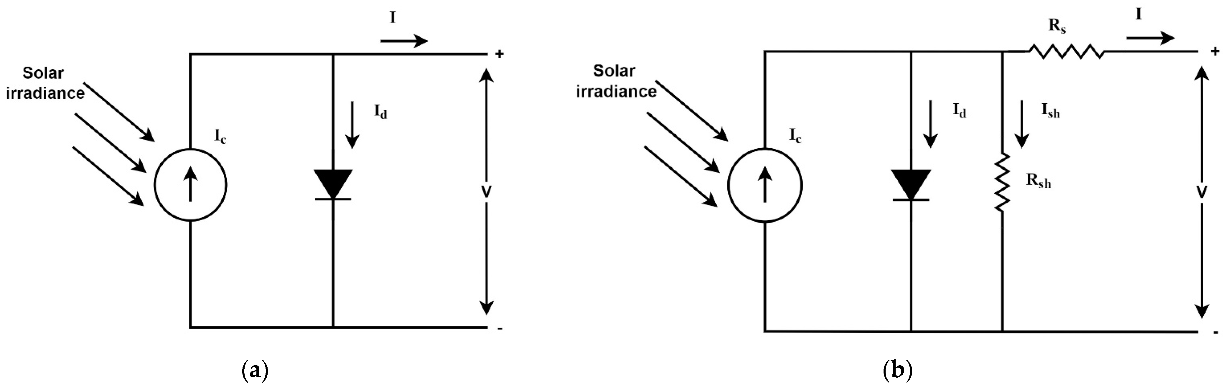
2. PV Models
2.1. SD Model
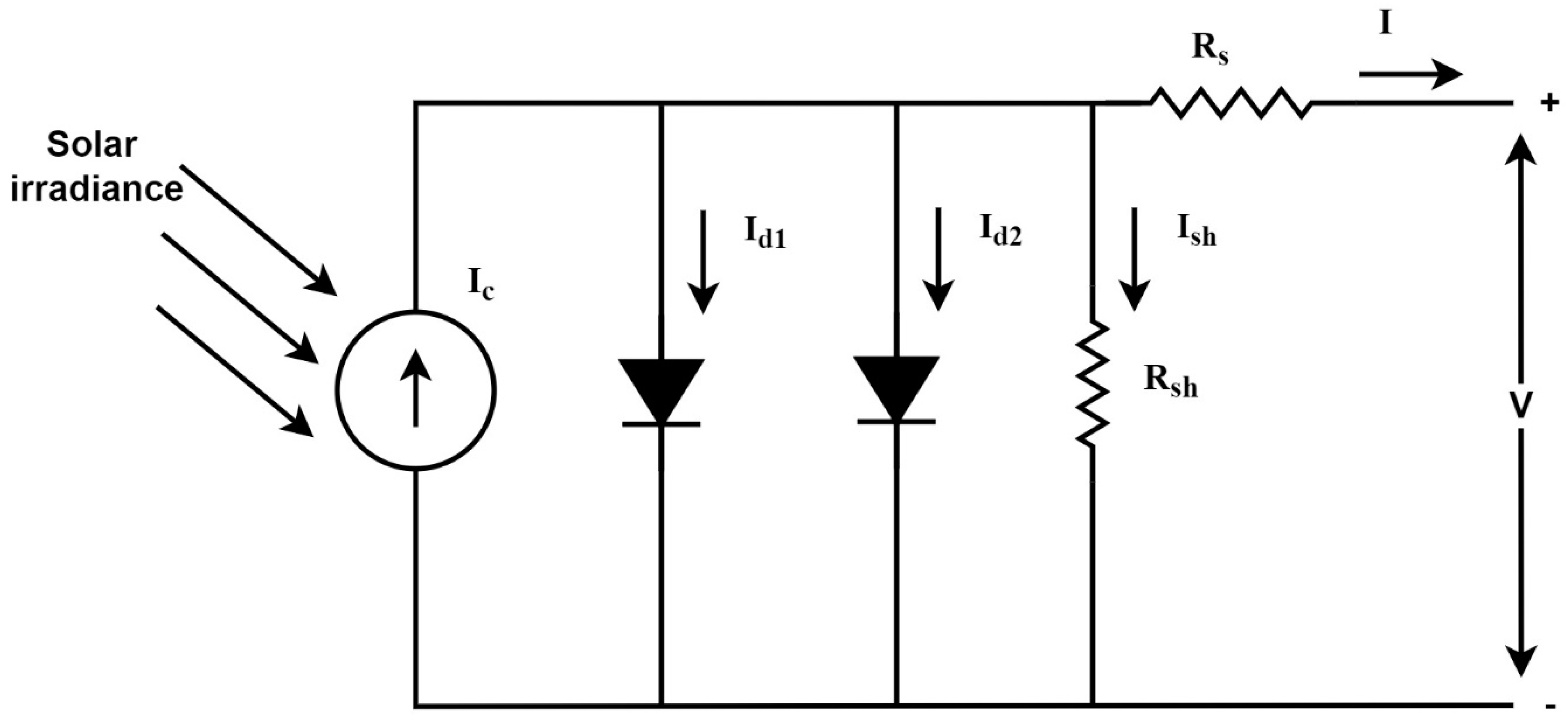
2.2. DD Model
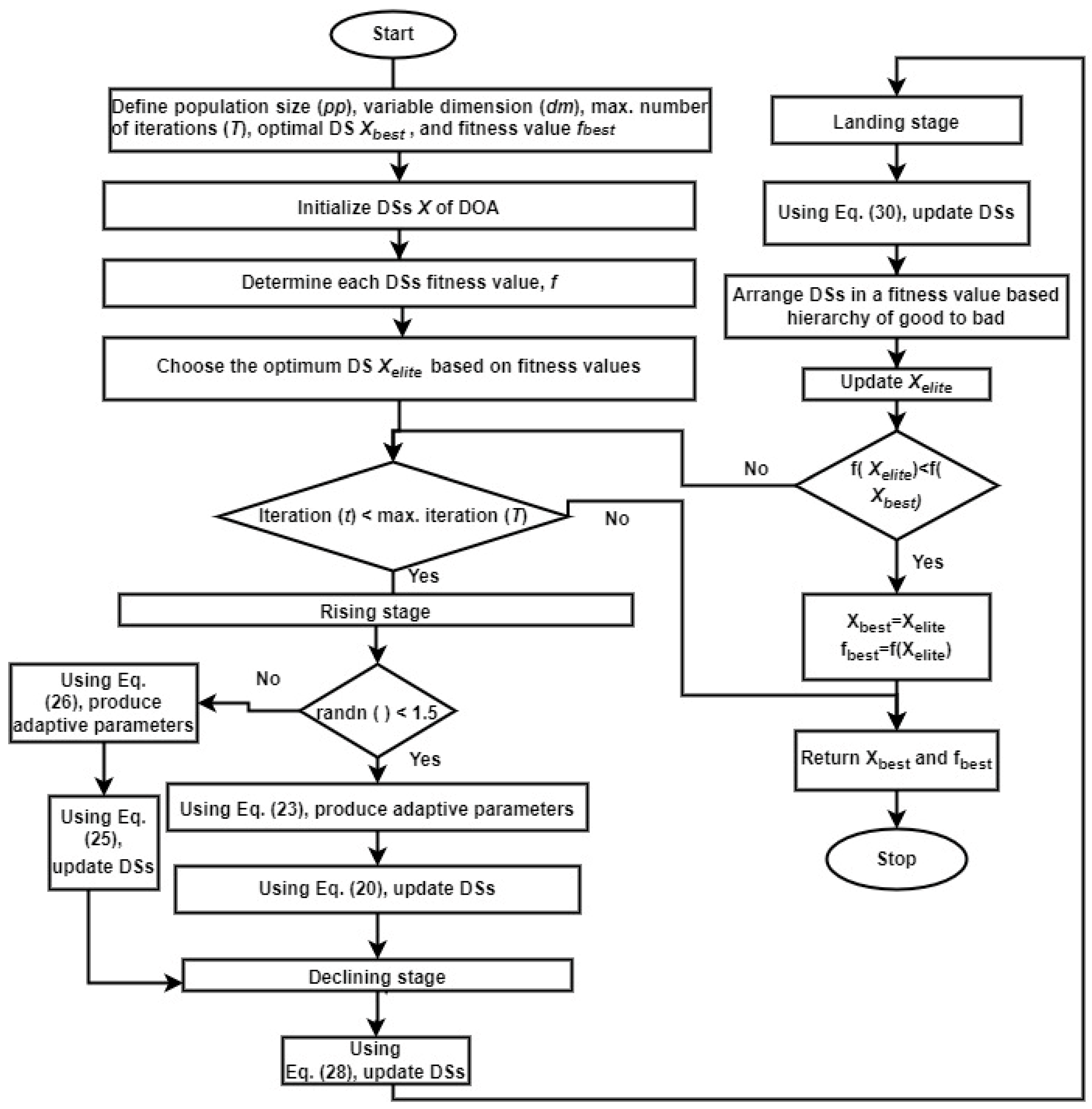
3. Dandelion Optimisation Algorithm
- When a DS is in the rising stage, a vortex is created above it, and it rises due to a pulling force under windy and bright conditions. In contrast, when it is raining, no eddies are above the seeds. In this situation, only local searches are possible.
- In the landing stage, DSs finally randomly settle in one location under the influence of wind and weather to create new dandelions.
- In the descending stage, once seeds soar up to a given height, they drop continuously.
3.1. Mathematical Formulation of the DOA
3.1.1. Rising Stage
3.1.2. Descending Stage
3.1.3. Landing Stage
4. Formulation of the Optimisation Problem
5. Procedural Steps for PV Module Parameter Estimation
- Step 1:
- Step 2:
- Verify the maximum iteration count before moving on to the next stages. If not, go to step 7.
- Step 3:
- Utilizing Equations (1)–(15), take into account the SD and DD models for the solar PV module under consideration.
- Step 4:
- Use Equations (16)–(31) to implement the suggested DOA for the research subject under consideration.
- Step 5:
- Reduce the net error given by Equations (35) and (39) for steps 3 and 4 for each iteration.
- Step 6:
- Count up the iterations and go on to step 2.
- Step 7:
- Completely analyse various solar PV modules and determine the best values for equivalent circuit parameters.
6. Results and Analysis

| Monocrystalline SF430M [40] | Polycrystalline SG350P [41] | Thin Film Shell ST40 [42] | |
|---|---|---|---|
| 41.2 V | 38.7 V | 16.60 V | |
| 10.44 A | 9.05 A | 2.41 A | |
| 49.4 V | 47.22 V | 23.30 V | |
| 11.06 A | 9.68 A | 2.68 A | |
| Temperature coefficient of | −0.37%/°C | −0.39%/°C | −0.6%/°C |
| Temperature coefficient of | −0.28%/°C | −0.28%/°C | −0.1%/°C |
| Temperature coefficient of | 0.042%/°C | 0.042%/°C | 0.00035%/°C |
| 72 | 72 | 36 |
| SD Model | DD Model | UPB | LOB |
|---|---|---|---|
| 2 | 0.5 | ||
| 1 | 0.001 | ||
| 200 | 50 | ||
| - | 10−12 | ||
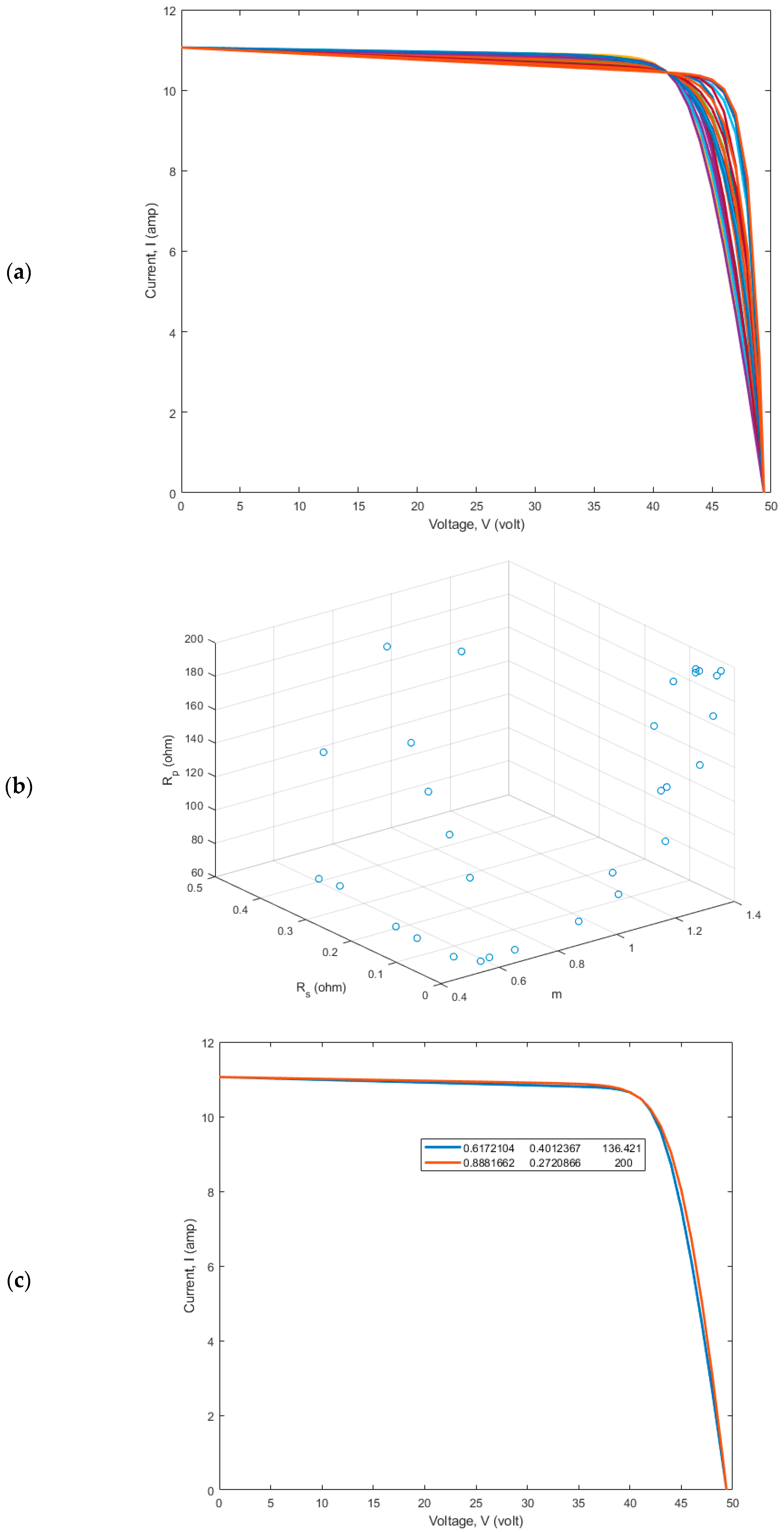
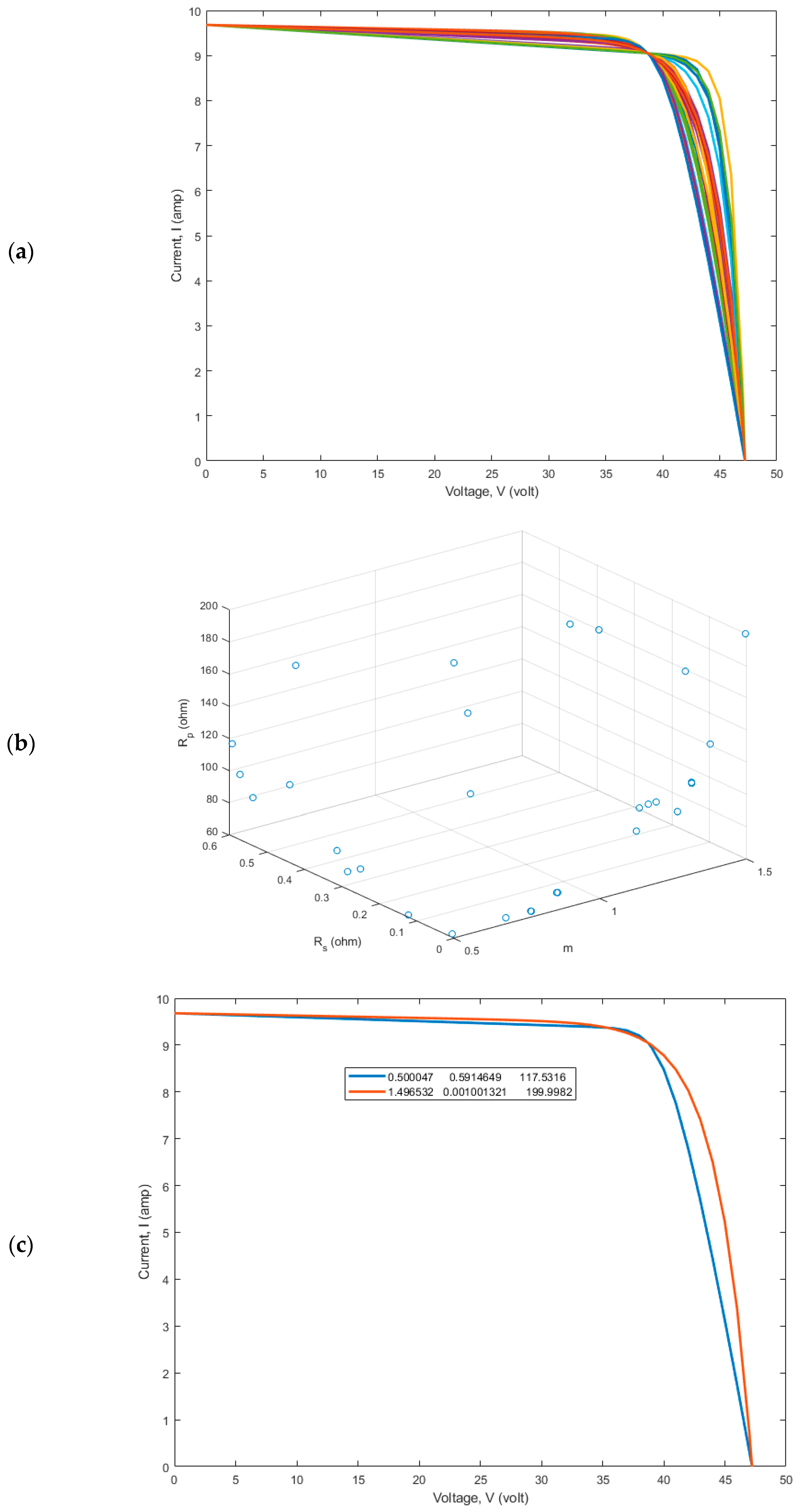
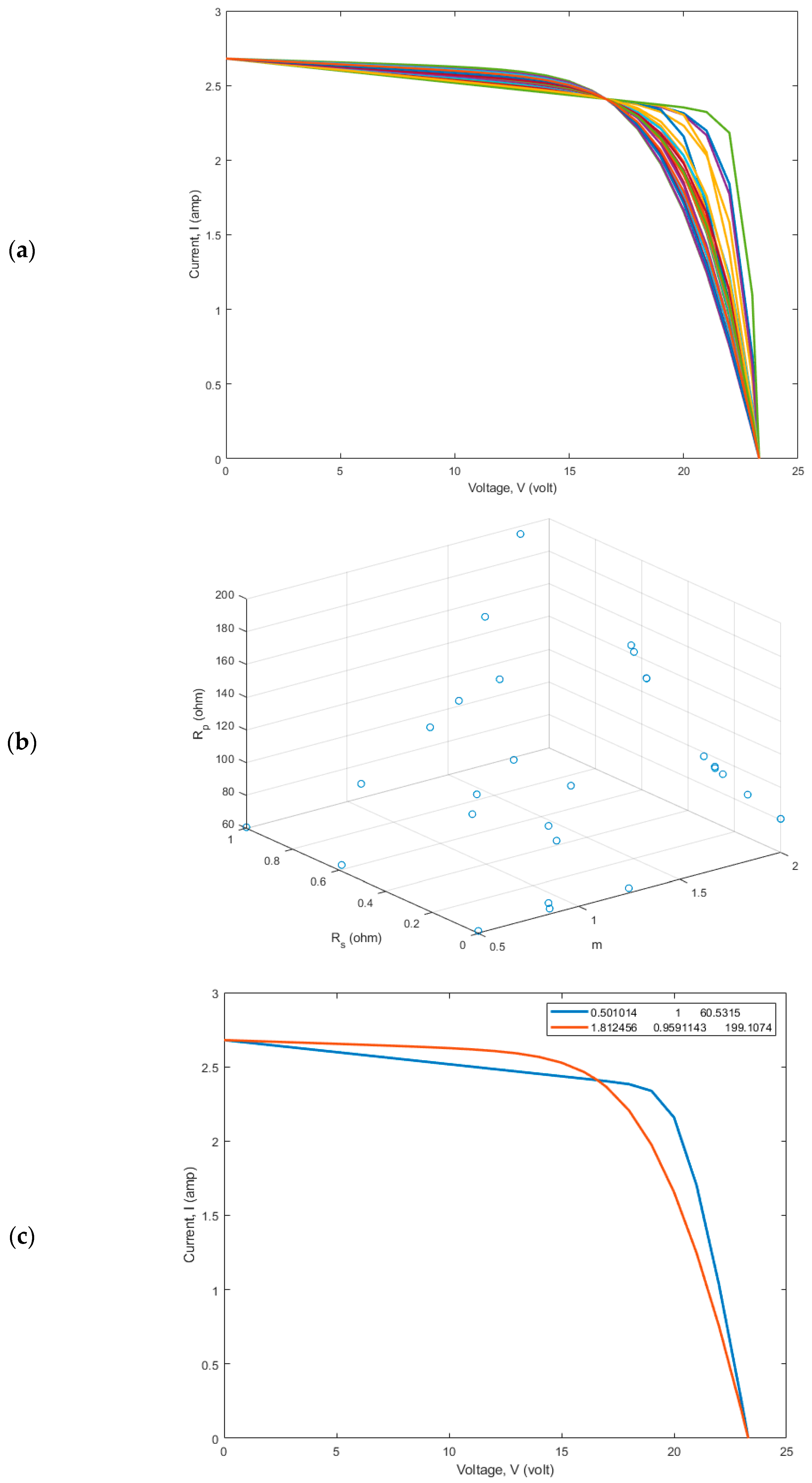
6.1. Parameter Estimation for SD Model of Various PV Panels


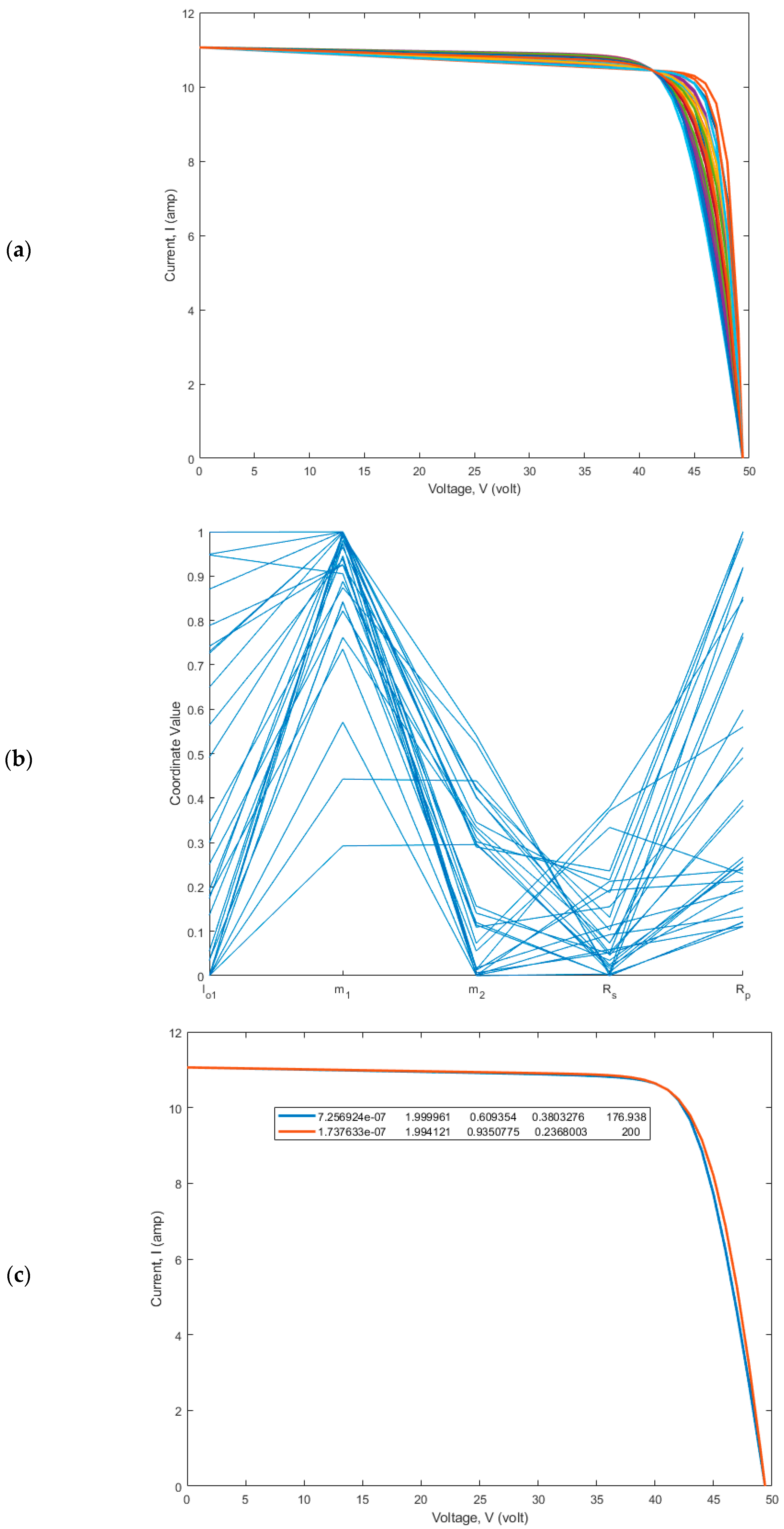
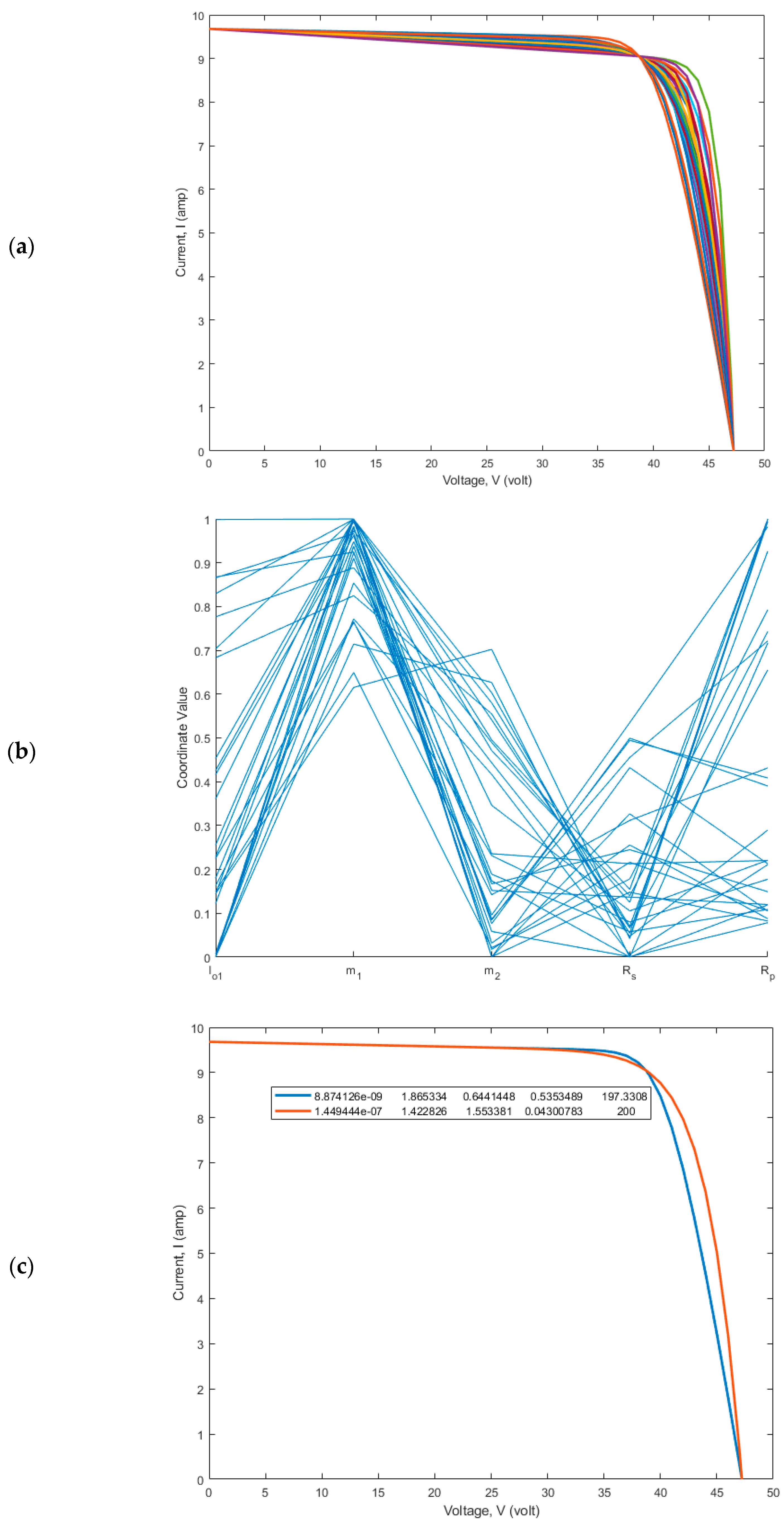
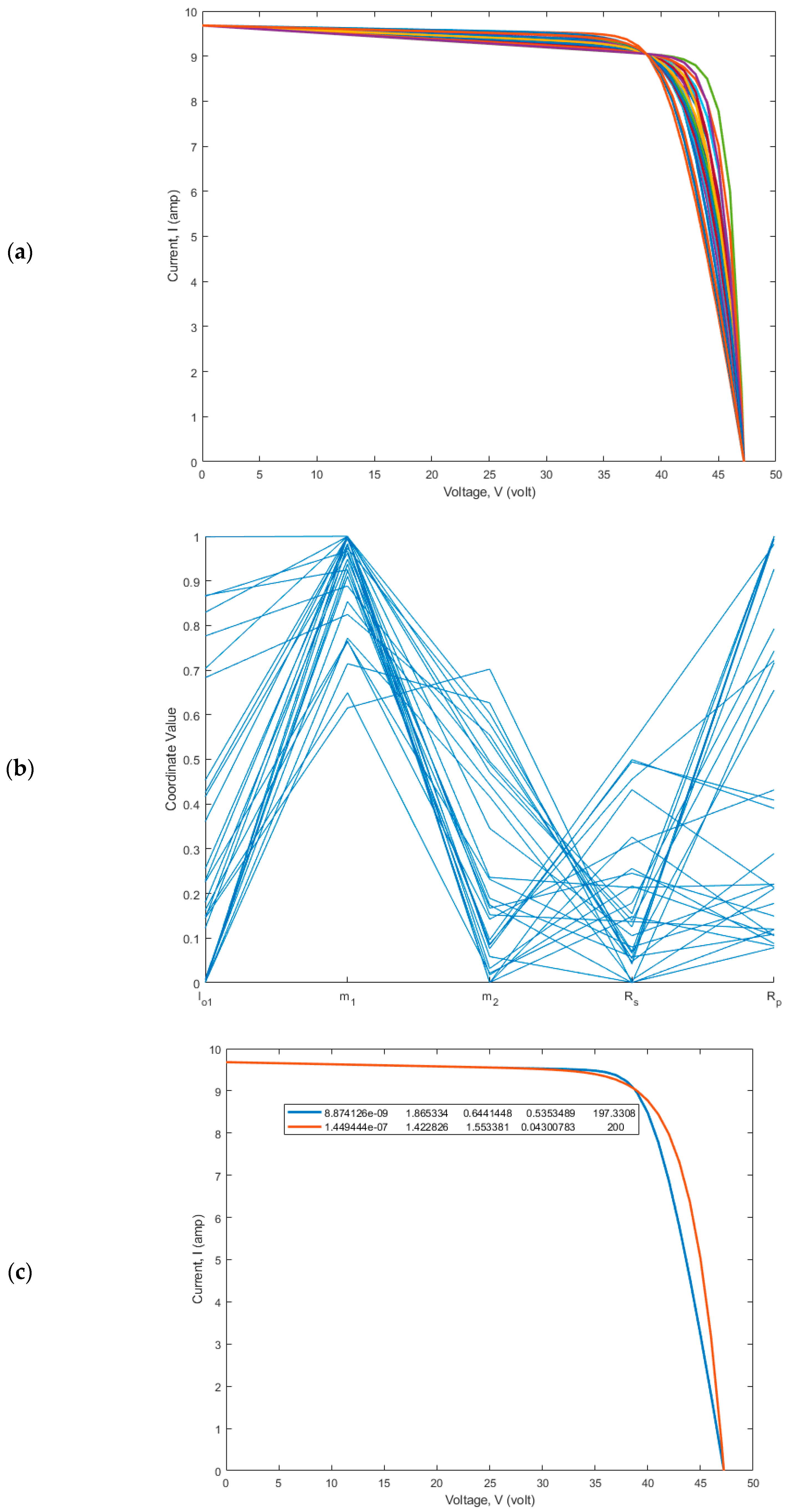
6.2. Parameter Estimation for DD Model of Various PV Panels


7. Conclusions
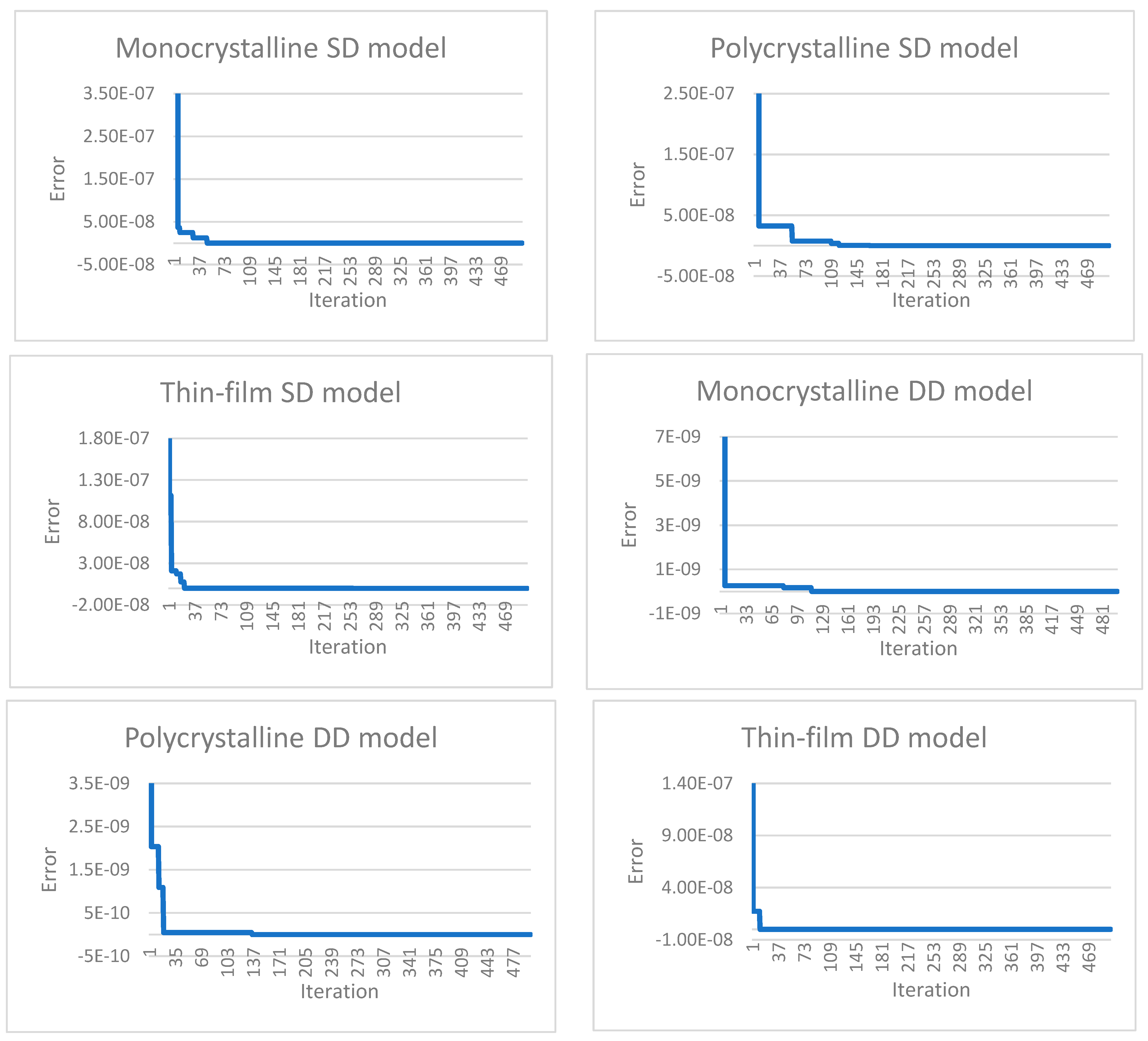
- The DOA yields more accurate results in over 30 trials with the specified error function as the objective function.
- The simulation findings show that the parameters estimated provide curves that pass through all three important points with approximately a 10e-22 error.
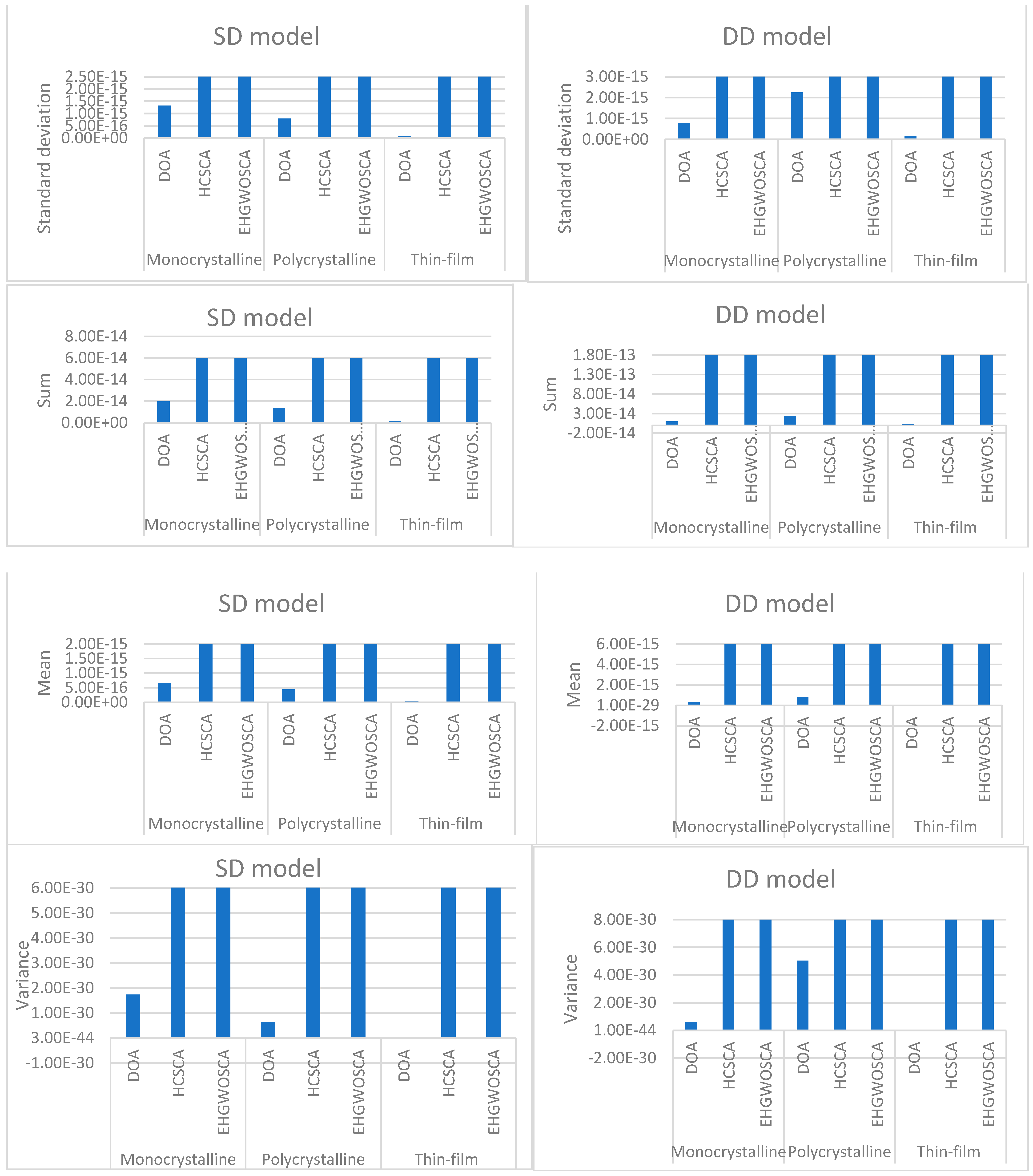
- A statistical evaluation of SD and DD models using the DOA has been performed and they have been compared with two hybrid OAs. From the statistical analysis, we can observe that the standard deviation, sum, mean, and variance of various PV panels using the DOA are lower compared with those using the other two hybrid OAs.
- The results show that the suggested algorithm produced adequate performance characteristics and that its practical ie was recommended.
Author Contributions
Funding
Institutional Review Board Statement
Informed Consent Statement
Data Availability Statement
Conflicts of Interest
References
- Esmaeili Shayan, M.; Najafi, G.; Ghobadian, B.; Gorjian, S.; Mazlan, M. Sustainable Design of a Near-Zero-Emissions Building Assisted by a Smart Hybrid Renewable Microgrid. Int. J. Renew. Energy Dev. 2022, 11, 471–480. [Google Scholar] [CrossRef]
- Esmaeili Shayan, M.; Najafi, G.; Esmaeili Shayan, S. Microgrids Energy Management System Based on Renewable Energy. Amirkabir J. Mech. Eng. 2023, 55, 1–10. [Google Scholar]
- Esmaeili Shayan, M.; Najafi, G.; Ghobadian, B.; Gorjian, S.; Mamat, R.; Fairusham Ghazali, M. Multi-microgrid optimization and energy management under boost voltage converter with Markov prediction chain and dynamic decision algorithm. Renew. Energy 2022, 201, 179–189. [Google Scholar] [CrossRef]
- Esmaeili Shayan, M.; Najafi, G.; Ghobadian, B.; Gorjian, S.; Mazlan, M.; Samami, M.; Shabanzadeh, A. Flexible Photovoltaic System on Non-Conventional Surfaces: A Techno-Economic Analysis. Sustainability 2022, 14, 3566. [Google Scholar] [CrossRef]
- Vandrasi, R.K.; Kumar, B.S.; Devarapalli, R. Solar photo voltaic module parameter extraction using a novel Hybrid Chimp-Sine Cosine Algorithm. Energy Sources Part A Recovery Util. Environ. Eff. 2022, 1–20. [Google Scholar] [CrossRef]
- Devarapalli, R.; Bathina, V.R.; Al-Durra, A. Optimal parameter assessment of Solar Photovoltaic module equivalent circuit using a novel enhanced hybrid GWO-SCA algorithm. Energy Rep. 2022, 8, 12282–12301. [Google Scholar] [CrossRef]
- Jordehi, A.R. Parameter estimation of solar photovoltaic (PV) cells: A review. Renew. Sustain. Energy Rev. 2016, 61, 354–371. [Google Scholar] [CrossRef]
- Bathina, V.R.; Devarapalli, R.; Malik, H.; Bali, S.K.; García Márquez, F.P.; Chiranjeevi, T. Wind integrated power system to reduce emission: An application of bat algorithm. J. Intell. Fuzzy Syst. 2022, 42, 1041–1049. [Google Scholar] [CrossRef]
- Chiranjeevi, T.; Gupta, U.K. Ideal parameter distribution in renewable integrated rapid charging electric vehicle station. Energy Sources Part A Recovery Util. Environ. Eff. 2023, 45, 888–904. [Google Scholar] [CrossRef]
- Knypiński, Ł.; Kuroczycki, S.; Marquez, F.P.G. Minimization of Torque Ripple in the Brushless DC Motor Using Constrained Cuckoo Search Algorithm. Electronics 2021, 10, 2299. [Google Scholar] [CrossRef]
- Jervase, J.A.; Bourdoucen, H.; Al-Lawati, A. Solar cell parameter extraction using genetic algorithms. Meas. Sci. Technol. 2001, 12, 1922. [Google Scholar] [CrossRef]
- Ye, M.; Wang, X.; Xu, Y. Parameter extraction of solar cells using particle swarm optimization. J. Appl. Phys. 2009, 105, 094502. [Google Scholar] [CrossRef]
- Bisht, R.; Sikander, A. A novel way of parameter estimation of solar photovoltaic system. COMPEL—Int. J. Comput. Math. Electr. Electron. Eng. 2022, 41, 471–498. [Google Scholar] [CrossRef]
- Naraharisetti, J.N.L.; Devarapalli, R.; Bathina, V. Parameter extraction of solar photovoltaic module by using a novel hybrid marine predators—Success history based adaptive differential evolution algorithm. Energy Sources Part A Recovery Util. Environ. Eff. 2020, 1–23. [Google Scholar] [CrossRef]
- Chen, X.; Yu, K. Hybridizing cuckoo search algorithm with biogeography-based optimization for estimating photovoltaic model parameters. Sol. Energy 2019, 180, 192–206. [Google Scholar] [CrossRef]
- AlHajri, M.; El-Naggar, K.; AlRashidi, M.; Al-Othman, A. Optimal extraction of solar cell parameters using pattern search. Renew. Energy 2012, 44, 238–245. [Google Scholar] [CrossRef]
- Sharma, A.; Dasgotra, A.; Tiwari, S.K.; Sharma, A.; Jately, V.; Azzopardi, B. Parameter Extraction of Photovoltaic Module Using Tunicate Swarm Algorithm. Electronics 2021, 10, 878. [Google Scholar] [CrossRef]
- Biswas, P.P.; Suganthan, P.N.; Wu, G.; Amaratunga, G.A.J. Parameter estimation of solar cells using datasheet information with the application of an adaptive differential evolution algorithm. Renew. Energy 2019, 132, 425–438. [Google Scholar] [CrossRef]
- Derick, M.; Rani, C.; Rajesh, M.; Farrag, M.; Wang, Y.; Busawon, K. An improved optimization technique for estimation of solar photovoltaic parameters. Sol. Energy 2017, 157, 116–124. [Google Scholar] [CrossRef]
- Repalle, N.B.; Sarala, P.; Mihet-Popa, L.; Kotha, S.R.; Rajeswaran, N. Implementation of a Novel Tabu Search Optimization Algorithm to Extract Parasitic Parameters of Solar Panel. Energies 2022, 15, 4515. [Google Scholar] [CrossRef]
- Singh, A.; Sharma, A.; Rajput, S.; Mondal, A.K.; Bose, A.; Ram, M. Parameter Extraction of Solar Module Using the Sooty Tern Optimization Algorithm. Electronics 2022, 11, 564. [Google Scholar] [CrossRef]
- Guo, L.; Meng, Z.; Sun, Y.; Wang, L. Parameter identification and sensitivity analysis of solar cell models with cat swarm optimization algorithm. Energy Convers. Manag. 2016, 108, 520–528. [Google Scholar] [CrossRef]
- Montoya, O.D.; Ramírez-Vanegas, C.A.; Grisales-Norena, L.F. Parametric estimation in photovoltaic modules using the crow search algorithm. Int. J. Electr. Comput. Eng. 2022, 12, 82–91. [Google Scholar] [CrossRef]
- Saxena, A.; Sharma, A.; Shekhawat, S. Parameter extraction of solar cell using intelligent grey wolf optimizer. Evol. Intell. 2022, 15, 167–183. [Google Scholar] [CrossRef]
- Louzazni, M.; Khouya, A.; Amechnoue, K.; Gandelli, A.; Mussetta, M.; Crăciunescu, A. Metaheuristic Algorithm for Photovoltaic Parameters: Comparative Study and Prediction with a Firefly Algorithm. Appl. Sci. 2018, 8, 339. [Google Scholar] [CrossRef]
- Oliva, D.; Cuevas, E.; Pajares, G. Parameter identification of solar cells using artificial bee colony optimization. Energy 2014, 72, 93–102. [Google Scholar] [CrossRef]
- Houssein, E.H.; Nageh, G.; Elaziz, M.A.; Younis, E. An efficient Equilibrium Optimizer for parameters identification of photovoltaic modules. PeerJ Comput. Sci. 2021, 7, e708. [Google Scholar] [CrossRef] [PubMed]
- Kashefi, H.; Sadegheih, A.; Mostafaeipour, A.; Mohammadpour Omran, M. Parameter identification of solar cells and fuel cell using improved social spider algorithm. COMPEL—Int. J. Comput. Math. Electr. Electron. Eng. 2021, 40, 142–172. [Google Scholar] [CrossRef]
- Abdel-Basset, M.; Mohamed, R.; El-Fergany, A.; Askar, S.S.; Abouhawwash, M. Efficient Ranking-Based Whale Optimizer for Parameter Extraction of Three-Diode Photovoltaic Model: Analysis and Validations. Energies 2021, 14, 3729. [Google Scholar] [CrossRef]
- Shaheen, A.; El-Sehiemy, R.; El-Fergany, A.; Ginidi, A. Representations of solar photovoltaic triple-diode models using artificial hummingbird optimizer. Energy Sources Part A Recovery Util. Environ. Eff. 2022, 44, 8787–8810. [Google Scholar] [CrossRef]
- Al-Shamma’a, A.A.; Omotoso, H.O.; Alturki, F.A.; Farh, H.M.H.; Alkuhayli, A.; Alsharabi, K.; Noman, A.M. Parameter Estimation of Photovoltaic Cell/Modules Using Bonobo Optimizer. Energies 2022, 15, 140. [Google Scholar] [CrossRef]
- Gao, X.; Cui, Y.; Hu, J.; Xu, G.; Yu, Y. Lambert W-function based exact representation for double diode model of solar cells: Comparison on fitness and parameter extraction. Energy Convers. Manag. 2016, 127, 443–460. [Google Scholar] [CrossRef]
- Chegaar, M.; Ouennoughi, Z.; Hoffmann, A. A new method for evaluating illuminated solar cell parameters. Solid-State Electron. 2001, 45, 293–296. [Google Scholar] [CrossRef]
- Reddy, S.S.; Yammani, C. Parameter extraction of single-diode photovoltaic module using experimental current–voltage data. Int. J. Circuit Theory Appl. 2021, 50, 753–771. [Google Scholar] [CrossRef]
- Louzazni, M.; Aroudam, E.H. An analytical mathematical modeling to extract the parameters of solar cell from implicit equation to explicit form. Appl. Sol. Energy 2015, 51, 165–171. [Google Scholar] [CrossRef]
- Muhammadsharif, F.F. A New Simplified Method for Efficient Extraction of Solar Cells and Modules Parameters from Datasheet Information. Silicon 2022, 14, 3059–3067. [Google Scholar] [CrossRef]
- Gong, C.; Han, S.; Li, X.; Zhao, L.; Liu, X. A new dandelion algorithm and optimization for extreme learning machine. J. Exp. Theor. Artif. Intell. 2018, 30, 39–52. [Google Scholar] [CrossRef]
- Li, X.; Han, S.; Zhao, L.; Gong, C.; Liu, X. New dandelion algorithm optimizes extreme learning machine for biomedical classification problems. Comput. Intell. Neurosci. 2017, 2017, 4523754. [Google Scholar] [CrossRef] [PubMed]
- Zhao, S.; Zhang, T.; Ma, S.; Chen, M. Dandelion Optimizer: A nature-inspired metaheuristic algorithm for engineering applications. Eng. Appl. Artif. Intell. 2022, 114, 105075. [Google Scholar] [CrossRef]
- SF430M Peimar Monocrystalline Solar Panels Datasheet. Available online: https://www.enfsolar.com/pv/panel-datasheet/crystalline/51664 (accessed on 1 July 2022).
- SG350P Peimar Polycrystalline Solar Panels Datasheet. Available online: https://www.enfsolar.com/pv/panel-datasheet/crystalline/51661 (accessed on 1 July 2022).
- Soon, J.J.; Low, K.S. Photovoltaic Model Identification Using Particle Swarm Optimization with Inverse Barrier Constraint. IEEE Trans. Power Electron. 2012, 27, 3975–3983. [Google Scholar] [CrossRef]


| Reference | Algorithm | Analytical Method | Metaheuristic Method | Model |
|---|---|---|---|---|
| [5] | Hybrid chimp–sine cosine algorithm | √ | SD and DD models | |
| [6] | Enhanced hybrid grey wolf optimiser–sine cosine algorithm | √ | SD and DD models | |
| [11] | Genetic algorithm | √ | DD model | |
| [12] | Particle swarm optimisation | √ | SD and DD models | |
| [13] | Jellyfish search | √ | SD model | |
| [14] | Hybrid differential evolution | √ | SD and DD models | |
| [15] | Cuckoo search with biogeography-based optimisation | √ | SD and DD models | |
| [16] | Pattern search | √ | SD and DD models | |
| [17] | Tunicate swarm | √ | SD model | |
| [18] | Differential evolution | √ | SD and DD models | |
| [19] | Harmony search | √ | SD and DD models | |
| [20] | Tabu search | √ | SD model | |
| [21] | Sooty tern | √ | SD model | |
| [22] | Cat swarm | √ | SD and DD models | |
| [23] | Crow search | √ | SD model | |
| [24] | Gray wolf optimiser | √ | SD and DD models | |
| [25] | Firefly algorithm | √ | SD and DD models | |
| [26] | Artificial bee colony | √ | SD and DD models | |
| [27] | Equilibrium optimiser | √ | SD and DD models | |
| [28] | Social spider algorithm | √ | SD and DD models | |
| [29] | Whale optimiser | √ | Triple diode (TD) model | |
| [30] | Humming bird optimiser | √ | TD model | |
| [31] | Bonobo optimiser | √ | SD and DD models | |
| [32] | Lambert W-functions | √ | DD model | |
| [33] | Conductivity method | √ | SD model | |
| [34] | Least squares | √ | SD model | |
| [35] | Analytical mathematical method | √ | SD model | |
| [36] | Iterative method | √ | SD model |
| Pseudo Code of DOA |
|---|
| Input variables: , , . Output variables: Optimal DS and its fitness value, . Initialise DSs’ of the DOA Determine each DSs’ fitness value, . Choose the optimum DS based on fitness values. while carry out /*Rising stage*/ if carry out By using Equation (23), produce adaptive parameters. By using Equation (20), update DSs. otherwise, carry out By using Equation (26), produce adaptive parameters. By using Equation (25), update DSs. end if /*Declining stage*/ By using Equation (28), update DSs. /*Landing stage*/ By using Equation (30), update DSs. Arrange DSs in a fitness value-based hierarchy of good to bad. Update if end if end while Return and . |
| Run | DOA | Analytical Method | ||||
|---|---|---|---|---|---|---|
| 1 | 0.5066 | 0.1687 | 67.4524 | 1.3264e-22 | 11.0876 | 2.0477e-17 |
| 2 | 1.2660 | 0.0490 | 192.0358 | 7.4668e-09 | 11.0628 | 3.2914e-16 |
| 3 | 0.8881 | 0.2720 | 200 | 9.4742e-13 | 11.0750 | 1.1424e-15 |
| 4 | 0.5713 | 0.0039 | 66.9424 | 5.1739e-20 | 11.0606 | 1.3270e-16 |
| 5 | 1.3555 | 0.0018 | 199.9999 | 3.0059e-08 | 11.0601 | 7.2251e-18 |
| 6 | 0.6542 | 0.0016 | 67.7582 | 1.9423e-17 | 11.0602 | 4.3208e-19 |
| 7 | 0.5034 | 0.1197 | 66.9729 | 9.4619e-23 | 11.0797 | 1.5614e-17 |
| 8 | 0.5002 | 0.0368 | 66.6534 | 6.7940e-23 | 11.0661 | 2.1375e-16 |
| 9 | 0.5371 | 0.0010 | 66.7436 | 2.6568e-21 | 11.0601 | 7.8490e-17 |
| 10 | 1.3274 | 0.0010 | 174.4444 | 1.9764e-08 | 11.0600 | 3.6750e-16 |
| 11 | 0.7852 | 0.2784 | 120.3921 | 1.8180e-14 | 11.0855 | 5.1414e-16 |
| 12 | 1.2109 | 0.0278 | 134.2327 | 2.8318e-09 | 11.0622 | 3.2215e-16 |
| 13 | 1.2172 | 0.0599 | 166.3733 | 3.1930e-09 | 11.0639 | 7.9023e-16 |
| 14 | 1.2826 | 0.0012 | 147.3545 | 9.7396e-09 | 11.0600 | 2.2499e-17 |
| 15 | 0.7910 | 0.2354 | 99.9845 | 2.3137e-14 | 11.0860 | 5.7332e-16 |
| 16 | 0.7712 | 0.1772 | 82.5875 | 9.6369e-15 | 11.0837 | 3.6795e-16 |
| 17 | 0.7539 | 0.3495 | 199.5575 | 4.4962e-15 | 11.0793 | 6.0320e-15 |
| 18 | 0.5042 | 0.3379 | 74.4950 | 1.0425e-22 | 11.1101 | 1.3074e-16 |
| 19 | 1.0320 | 0.0311 | 91.5428 | 6.0852e-11 | 11.0637 | 7.1674e-18 |
| 20 | 0.7755 | 0.3104 | 145.9505 | 1.1957e-14 | 11.0835 | 8.2083e-17 |
| 21 | 0.5258 | 0.3054 | 73.2910 | 9.2226e-22 | 11.1060 | 2.7147e-16 |
| 22 | 1.1985 | 0.0324 | 132.1643 | 2.2530e-09 | 11.0627 | 7.9011e-16 |
| 23 | 1.1650 | 0.0010 | 107.6268 | 1.1776e-09 | 11.0601 | 6.5412e-16 |
| 24 | 1.3158 | 0.0242 | 199.0640 | 1.6608e-08 | 11.0613 | 1.0871e-17 |
| 25 | 0.6172 | 0.4012 | 136.4209 | 1.7383e-18 | 11.0925 | 4.7216e-15 |
| 26 | 1.3098 | 0.0281 | 199.9976 | 1.5139e-08 | 11.0615 | 1.2625e-15 |
| 27 | 1.3465 | 0.0053 | 197.1366 | 2.6373e-08 | 11.0602 | 8.4918e-18 |
| 28 | 1.0055 | 0.0010 | 83.7745 | 3.0648e-11 | 11.0601 | 2.5118e-19 |
| 29 | 1.3087 | 0.0277 | 197.9710 | 1.4874e-08 | 11.0615 | 6.2800e-18 |
| 30 | 0.8707 | 0.0011 | 74.1570 | 4.9832e-13 | 11.0601 | 9.2189e-16 |
| Run | DOA | Analytical Method | ||||
|---|---|---|---|---|---|---|
| 1 | 1.1646 | 0.2096 | 199.9853 | 2.8627e-09 | 9.6901 | 1.4939e-15 |
| 2 | 1.1653 | 0.0330 | 90.4115 | 2.8122e-09 | 9.6835 | 9.3348e-17 |
| 3 | 0.6375 | 0.5293 | 166.0917 | 3.8465e-17 | 9.7108 | 4.7089e-16 |
| 4 | 0.5844 | 0.3777 | 70.0374 | 9.7381e-19 | 9.7322 | 2.9725e-17 |
| 5 | 0.9470 | 0.3123 | 144.4529 | 1.8440e-11 | 9.7009 | 1.3180e-16 |
| 6 | 1.2380 | 0.0372 | 104.2750 | 1.0256e-08 | 9.6834 | 6.6337e-17 |
| 7 | 0.7656 | 0.0010 | 63.6454 | 2.9652e-14 | 9.6801 | 1.3493e-15 |
| 8 | 1.2212 | 0.0449 | 102.9439 | 7.7210e-09 | 9.6842 | 3.9785e-17 |
| 9 | 0.5007 | 0.5712 | 100.5910 | 6.7232e-22 | 9.7349 | 1.3128e-17 |
| 10 | 0.5058 | 0.0089 | 61.5251 | 1.0856e-21 | 9.6814 | 8.6616e-18 |
| 11 | 1.3712 | 0.0634 | 176.1996 | 7.7475e-08 | 9.6834 | 3.5573e-16 |
| 12 | 0.8829 | 0.0219 | 67.2878 | 2.5012e-12 | 9.6831 | 9.4824e-21 |
| 13 | 0.5839 | 0.5035 | 97.3535 | 9.5643e-19 | 9.7300 | 3.8534e-15 |
| 14 | 0.9045 | 0.2719 | 100.6567 | 5.1312e-12 | 9.7061 | 2.9987e-19 |
| 15 | 0.5000 | 0.1212 | 61.5931 | 6.0347e-22 | 9.6990 | 2.7429e-18 |
| 16 | 0.5482 | 0.3212 | 64.7611 | 5.4297e-20 | 9.7280 | 2.9782e-17 |
| 17 | 1.2184 | 0.1745 | 197.5454 | 7.5298e-09 | 9.6885 | 2.0915e-18 |
| 18 | 1.2666 | 0.0027 | 100.5927 | 1.6296e-08 | 9.6802 | 2.5461e-16 |
| 19 | 0.9359 | 0.3406 | 173.1933 | 1.3469e-11 | 9.6990 | 8.7728e-17 |
| 20 | 0.8806 | 0.0233 | 67.2490 | 2.3198e-12 | 9.6833 | 5.1891e-18 |
| 21 | 1.2004 | 0.0526 | 100.7845 | 5.3659e-09 | 9.6850 | 2.9264e-16 |
| 22 | 0.7652 | 0.0023 | 63.6575 | 2.9201e-14 | 9.6803 | 7.3543e-16 |
| 23 | 1.4965 | 0.0010 | 199.9981 | 3.6934e-07 | 9.6800 | 1.1224e-16 |
| 24 | 0.5805 | 0.3121 | 65.8014 | 7.2393e-19 | 9.7259 | 2.9825e-16 |
| 25 | 0.5083 | 0.5426 | 88.8710 | 1.4328e-21 | 9.7391 | 5.9047e-16 |
| 26 | 0.6885 | 0.0087 | 62.5949 | 7.1022e-16 | 9.6813 | 3.4635e-17 |
| 27 | 1.3219 | 0.0081 | 114.8555 | 3.8116e-08 | 9.6806 | 1.8545e-15 |
| 28 | 1.3854 | 0.0081 | 136.1256 | 9.2943e-08 | 9.6805 | 3.9759e-19 |
| 29 | 0.5000 | 0.5914 | 117.5315 | 6.3105e-22 | 9.7287 | 1.1503e-15 |
| 30 | 1.3227 | 0.0089 | 115.4072 | 3.8580e-08 | 9.6807 | 3.4042e-17 |
| Run | DOA | Analytical Method | ||||
|---|---|---|---|---|---|---|
| 1 | 0.8755 | 0.0196 | 61.6039 | 7.3527e-13 | 2.6808 | 6.7055e-17 |
| 2 | 1.9964 | 0.2813 | 93.6305 | 8.0806e-06 | 2.6880 | 3.6331e-19 |
| 3 | 1.2467 | 0.0010 | 63.1023 | 3.8777e-09 | 2.6800 | 1.7621e-20 |
| 4 | 1.9999 | 0.5795 | 129.3084 | 8.5035e-06 | 2.6920 | 1.2099e-18 |
| 5 | 1.3212 | 0.7201 | 71.6375 | 1.2499e-08 | 2.7069 | 1.9623e-17 |
| 6 | 1.5900 | 0.5486 | 79.1210 | 3.1651e-07 | 2.6985 | 3.4663e-17 |
| 7 | 1.9994 | 0.2500 | 91.8552 | 8.2144e-06 | 2.6872 | 1.4853e-17 |
| 8 | 2 | 0.6332 | 141.8301 | 8.5618e-06 | 2.6919 | 9.1611e-19 |
| 9 | 1.2218 | 0.6531 | 67.1147 | 2.6236e-09 | 2.7060 | 9.8823e-18 |
| 10 | 1.3678 | 0.4519 | 68.0710 | 2.3658e-08 | 2.6977 | 7.7787e-18 |
| 11 | 0.9102 | 0.0544 | 61.6420 | 2.2034e-12 | 2.6823 | 1.1614e-17 |
| 12 | 1.8124 | 0.9591 | 199.1073 | 2.3699e-06 | 2.6929 | 8.5869e-17 |
| 13 | 1.9999 | 0.0010 | 80.5765 | 8.0980e-06 | 2.6800 | 5.0441e-18 |
| 14 | 1.0698 | 0.9999 | 68.3693 | 1.4132e-10 | 2.7191 | 2.4169e-19 |
| 15 | 0.5010 | 1 | 60.5315 | 3.4096e-22 | 2.7242 | 4.8679e-16 |
| 16 | 2 | 0.0010 | 80.5767 | 8.0983e-06 | 2.6800 | 1.7172e-16 |
| 17 | 0.5341 | 0.6183 | 60.8769 | 7.6567e-21 | 2.7072 | 9.2716e-17 |
| 18 | 1.6829 | 0.9989 | 150.2686 | 8.0317e-07 | 2.6978 | 1.0543e-18 |
| 19 | 0.5006 | 0.0010 | 61.4807 | 3.2193e-22 | 2.6800 | 2.8472e-18 |
| 20 | 1.9993 | 0.0010 | 80.5456 | 8.0632e-06 | 2.6800 | 7.4597e-20 |
| 21 | 1.9999 | 0.1435 | 86.1606 | 8.1721e-06 | 2.6844 | 2.7141e-19 |
| 22 | 1.6548 | 0.9116 | 118.6317 | 6.1330e-07 | 2.7005 | 2.3453e-16 |
| 23 | 1.9992 | 0.3316 | 97.5556 | 8.2591e-06 | 2.6891 | 6.2520e-17 |
| 24 | 1.3149 | 0.3712 | 65.9451 | 1.1203e-08 | 2.6950 | 2.0376e-18 |
| 25 | 1.5301 | 0.7428 | 84.3621 | 1.7192e-07 | 2.7035 | 4.3950e-17 |
| 26 | 2 | 0.2850 | 94.1917 | 8.2672e-06 | 2.6881 | 4.9402e-18 |
| 27 | 1.9999 | 0.6453 | 145.1735 | 8.5738e-06 | 2.6919 | 1.2349e-17 |
| 28 | 1.4116 | 0.9999 | 91.6732 | 4.3676e-08 | 2.7092 | 6.4730e-17 |
| 29 | 1.5287 | 0.9777 | 105.4428 | 1.7321e-07 | 2.7048 | 3.5642e-18 |
| 30 | 1.9999 | 0.5789 | 129.1812 | 8.5042e-06 | 2.6920 | 3.5939e-17 |
| Run | DOA | Analytical Method | ||||||
|---|---|---|---|---|---|---|---|---|
| 1 | 1.9995 | 0.5011 | 0.2134 | 85.7834 | 9.9900e-07 | 7.1045e-23 | 11.0875 | 1.3680e-19 |
| 2 | 1.9941 | 0.9350 | 0.2368 | 200 | 1.7376e-07 | 4.2362e-12 | 11.0730 | 3.5206e-19 |
| 3 | 1.9990 | 0.9463 | 0.0170 | 88.6811 | 7.2968e-07 | 5.5871e-12 | 11.0621 | 1.6737e-19 |
| 4 | 1.9831 | 0.7116 | 0.0507 | 73.0153 | 3.0009e-07 | 5.1353e-16 | 11.0676 | 2.0463e-22 |
| 5 | 1.9705 | 1.0186 | 0.1882 | 187.9229 | 5.5469e-08 | 4.4296e-11 | 11.0710 | 8.8287e-19 |
| 6 | 1.9999 | 0.6093 | 0.3803 | 176.9380 | 7.2569e-07 | 9.5962e-19 | 11.0837 | 1.6842e-16 |
| 7 | 0.9387 | 0.9433 | 0.0219 | 80.4309 | 1.0000e-12 | 4.1537e-12 | 11.0630 | 2.9206e-16 |
| 8 | 1.7637 | 0.5832 | 0.3348 | 84.4166 | 1.0000e-12 | 1.3681e-19 | 11.1038 | 3.2421e-16 |
| 9 | 2 | 0.5183 | 0.1934 | 81.9717 | 8.7052e-07 | 4.1912e-22 | 11.0861 | 1.7695e-16 |
| 10 | 1.9474 | 0.9676 | 0.0086 | 88.5960 | 4.9116e-07 | 1.0402e-11 | 11.0610 | 8.2954e-16 |
| 11 | 1.9990 | 0.5264 | 0.1129 | 78.6888 | 9.4928e-07 | 9.1653e-22 | 11.0758 | 2.9086e-17 |
| 12 | 1.9874 | 1.3112 | 0.0010 | 164.3995 | 3.3751e-08 | 1.5345e-08 | 11.0600 | 4.7554e-18 |
| 13 | 1.7323 | 1.0026 | 0.0751 | 127.0942 | 2.5112e-07 | 2.5595e-11 | 11.0665 | 1.8711e-16 |
| 14 | 1.7614 | 0.6797 | 0.0010 | 68.1359 | 2.0044e-12 | 8.9493e-17 | 11.0601 | 1.0901e-16 |
| 15 | 2 | 0.6713 | 0.0015 | 68.0090 | 1.0088e-12 | 5.4977e-17 | 11.0602 | 1.0573e-16 |
| 16 | 1.3563 | 0.5015 | 0.0598 | 66.7099 | 1.0826e-12 | 7.7550e-23 | 11.0699 | 3.8492e-16 |
| 17 | 1.8579 | 0.6638 | 0.1562 | 123.6696 | 9.4765e-07 | 3.0473e-17 | 11.0739 | 6.8046e-17 |
| 18 | 1.8319 | 0.9528 | 0.2162 | 197.7403 | 1.3632e-07 | 7.0970e-12 | 11.0720 | 4.6200e-17 |
| 19 | 1.6426 | 0.9898 | 0.0255 | 90.0449 | 3.5376e-08 | 1.9408e-11 | 11.0631 | 1.5991e-16 |
| 20 | 1.6029 | 0.5095 | 0.0526 | 107.4908 | 1.8031e-07 | 1.2991e-22 | 11.0654 | 4.1592e-15 |
| 21 | 1.8880 | 1.1372 | 0.0525 | 165.7020 | 7.4178e-07 | 6.1687e-10 | 11.0635 | 1.7752e-15 |
| 22 | 1.8109 | 1.2843 | 0.0065 | 187.9730 | 3.4398e-07 | 9.2667e-09 | 11.0603 | 5.5379e-16 |
| 23 | 1.9597 | 0.5000 | 0.0047 | 66.6119 | 1.0438e-12 | 6.5820e-23 | 11.0607 | 1.9587e-17 |
| 24 | 1.8886 | 0.7354 | 0.0353 | 86.8116 | 7.8832e-07 | 1.5982e-15 | 11.0645 | 3.0808e-17 |
| 25 | 2 | 1.1299 | 0.1322 | 200 | 1.5061e-10 | 5.8883e-10 | 11.0673 | 2.6998e-16 |
| 26 | 1.1637 | 1.1580 | 0.1035 | 177.9818 | 4.4891e-12 | 1.0385e-09 | 11.0664 | 2.1860e-17 |
| 27 | 1.9179 | 0.5033 | 0.0934 | 70.0183 | 1.9303e-07 | 9.2160e-23 | 11.0747 | 4.6731e-19 |
| 28 | 1.9962 | 1.1017 | 0.0743 | 139.7824 | 6.4939e-07 | 3.0600e-10 | 11.0658 | 3.5561e-17 |
| 29 | 1.9077 | 0.5204 | 0.3728 | 133.9937 | 5.6407e-07 | 5.2070e-22 | 11.0907 | 5.5428e-16 |
| 30 | 1.9965 | 1.1041 | 0.0468 | 109.3303 | 1.0491e-12 | 3.3271e-10 | 11.0647 | 3.5995e-17 |
| Run | DOA | Analytical Method | ||||||
|---|---|---|---|---|---|---|---|---|
| 1 | 1.6576 | 1.1248 | 0.0069 | 81.6958 | 1.0000e-12 | 1.2698e-09 | 9.6808 | 2.8303e-20 |
| 2 | 1.9906 | 0.8543 | 0.2141 | 83.0836 | 4.2553e-07 | 9.4815e-13 | 9.7049 | 5.1853e-17 |
| 3 | 1.9991 | 1.4048 | 0.0448 | 199.1375 | 8.2938e-07 | 1.1759e-07 | 9.6821 | 3.6797e-16 |
| 4 | 1.9748 | 0.5000 | 0.3272 | 65.7817 | 2.5592e-07 | 5.9983e-22 | 9.7281 | 3.5763e-18 |
| 5 | 1.9064 | 0.5879 | 0.0019 | 61.7913 | 2.2285e-09 | 1.2414e-18 | 9.6802 | 4.8951e-17 |
| 6 | 1.9998 | 0.7282 | 0.1379 | 68.0113 | 4.5339e-07 | 5.2963e-15 | 9.6996 | 2.8251e-16 |
| 7 | 1.9999 | 1.0190 | 0.1063 | 83.1975 | 2.2911e-10 | 1.2078e-10 | 9.6923 | 1.4634e-15 |
| 8 | 1.5716 | 1.4399 | 0.0010 | 157.4846 | 5.6125e-10 | 1.8746e-07 | 9.6800 | 2.1316e-15 |
| 9 | 1.8653 | 0.6441 | 0.5353 | 197.3307 | 8.8741e-09 | 5.8293e-17 | 9.7062 | 7.2147e-16 |
| 10 | 1.9704 | 0.6267 | 0.4949 | 111.2720 | 1.4728e-11 | 1.9082e-17 | 9.7230 | 7.2748e-16 |
| 11 | 1.6477 | 0.7135 | 0.3122 | 114.7205 | 2.2562e-07 | 2.3532e-15 | 9.7063 | 4.9865e-16 |
| 12 | 1.7373 | 1.3321 | 0.0551 | 199.8697 | 6.8321e-07 | 3.7210e-08 | 9.6826 | 1.3725e-17 |
| 13 | 1.8840 | 0.7507 | 0.2461 | 72.4010 | 2.9376e-11 | 1.5532e-14 | 9.7129 | 2.1134e-20 |
| 14 | 1.6456 | 0.8476 | 0.0809 | 76.6722 | 1.6312e-07 | 6.8326e-13 | 9.6902 | 1.3079e-18 |
| 15 | 1.9994 | 0.6146 | 0.4998 | 108.5198 | 3.2942e-12 | 8.5399e-18 | 9.7245 | 1.6354e-16 |
| 16 | 1.9598 | 1.3700 | 0.0710 | 188.9893 | 1.2227e-07 | 7.5924e-08 | 9.6836 | 5.3382e-18 |
| 17 | 1.9999 | 0.5478 | 0.2567 | 63.1606 | 1.0011e-12 | 5.2160e-20 | 9.7193 | 1.3152e-17 |
| 18 | 2 | 1.3115 | 0.0673 | 148.3423 | 3.6112e-07 | 3.2618e-08 | 9.6843 | 1.4973e-16 |
| 19 | 1.4739 | 0.5323 | 0.1791 | 168.9302 | 1.5029e-07 | 6.5953e-21 | 9.6902 | 1.1615e-14 |
| 20 | 1.9225 | 0.7838 | 0.0588 | 66.3288 | 1.8026e-07 | 6.3978e-14 | 9.6885 | 4.9555e-17 |
| 21 | 1.9432 | 0.5265 | 0.2173 | 65.8755 | 4.1640e-07 | 7.7455e-21 | 9.7119 | 6.1819e-17 |
| 22 | 2 | 0.5001 | 0.4326 | 81.9582 | 9.9875e-07 | 5.9915e-22 | 9.7311 | 9.3837e-18 |
| 23 | 1.9498 | 0.7612 | 0.0010 | 67.8896 | 8.6552e-07 | 2.3430e-14 | 9.6801 | 1.7277e-18 |
| 24 | 1.7804 | 1.1646 | 0.0484 | 93.4726 | 6.3280e-09 | 2.7793e-09 | 9.6850 | 3.3843e-18 |
| 25 | 2 | 0.5013 | 0.1490 | 62.3844 | 1.4445e-07 | 6.8580e-22 | 9.7031 | 3.2879e-17 |
| 26 | 2 | 1.2065 | 0.1408 | 161.4284 | 7.0345e-07 | 5.9391e-09 | 9.6884 | 1.8631e-18 |
| 27 | 1.9981 | 1.2430 | 0.1555 | 199.9746 | 2.2934e-07 | 1.1303e-08 | 9.6875 | 7.7431e-16 |
| 28 | 1.8329 | 1.2342 | 0.1258 | 199.9587 | 7.7650e-07 | 8.9471e-09 | 9.6860 | 4.1349e-19 |
| 29 | 1.4228 | 1.5533 | 0.0430 | 200 | 1.4494e-07 | 3.4957e-08 | 9.6820 | 5.2704e-15 |
| 30 | 1.8869 | 0.6304 | 0.4559 | 158.2097 | 8.6741e-07 | 2.2883e-17 | 9.7078 | 2.9661e-16 |
| Run | DOA | Analytical Method | ||||||
|---|---|---|---|---|---|---|---|---|
| 1 | 1.5337 | 0.5224 | 0.9630 | 60.6195 | 2.8984e-10 | 2.6833e-21 | 2.7225 | 2.9122e-19 |
| 2 | 1.9950 | 1.9695 | 0.2862 | 91.7166 | 1.5122e-08 | 6.7733e-06 | 2.6883 | 1.6850e-19 |
| 3 | 1.5738 | 0.9588 | 0.2969 | 64.9617 | 9.5282e-08 | 5.7604e-12 | 2.6922 | 1.4021e-19 |
| 4 | 1.7927 | 1.2757 | 0.8267 | 90.1395 | 8.5012e-07 | 3.6404e-09 | 2.7045 | 7.8745e-18 |
| 5 | 1.7581 | 1.6149 | 0.7695 | 96.0318 | 1.7189e-07 | 3.6506e-07 | 2.7014 | 5.4478e-17 |
| 6 | 1.7006 | 1.6202 | 0.6361 | 86.4797 | 1.7810e-07 | 3.4442e-07 | 2.6997 | 7.9361e-22 |
| 7 | 1.7268 | 1.9671 | 0.6621 | 139.2834 | 1.4930e-08 | 6.8429e-06 | 2.6927 | 1.5140e-17 |
| 8 | 1.8625 | 2 | 0.7590 | 189.6899 | 9.8681e-08 | 8.4479e-06 | 2.6907 | 3.0559e-17 |
| 9 | 1.9609 | 0.5022 | 0.2818 | 62.4350 | 3.8901e-07 | 3.5835e-22 | 2.6920 | 2.8063e-17 |
| 10 | 1.4998 | 1.3868 | 0.7457 | 77.8482 | 4.6590e-08 | 1.9246e-08 | 2.7056 | 1.4370e-18 |
| 11 | 1.9999 | 1.2008 | 0.2011 | 63.5729 | 1.2148e-07 | 1.7740e-09 | 2.6884 | 2.1936e-17 |
| 12 | 1.7096 | 0.5011 | 0.2120 | 61.2789 | 7.6222e-10 | 3.4104e-22 | 2.6892 | 7.9437e-19 |
| 13 | 1.9896 | 0.5933 | 0.4116 | 61.1869 | 3.1508e-08 | 8.4217e-19 | 2.6980 | 4.0059e-17 |
| 14 | 1.9815 | 1.1111 | 0.3436 | 64.3788 | 4.7572e-07 | 3.1011e-10 | 2.6943 | 9.2057e-18 |
| 15 | 1.8152 | 1.4450 | 0.0141 | 68.2482 | 8.4748e-07 | 3.8618e-08 | 2.6805 | 6.7612e-19 |
| 16 | 2 | 2 | 0.3566 | 99.7046 | 1.2391e-07 | 8.1947e-06 | 2.6895 | 1.1594e-16 |
| 17 | 1.8557 | 1.3175 | 0.0023 | 65.6913 | 6.1106e-07 | 9.1759e-09 | 2.6800 | 1.0629e-18 |
| 18 | 1.5496 | 1.9748 | 0.2055 | 87.3912 | 1.3397e-09 | 6.9365e-06 | 2.6863 | 5.0120e-19 |
| 19 | 1.6816 | 1.4256 | 0.9895 | 139.7725 | 7.2838e-07 | 4.2003e-09 | 2.6989 | 4.2693e-21 |
| 20 | 1.6349 | 1.2090 | 0.0032 | 63.6576 | 7.3524e-08 | 1.7453e-09 | 2.6801 | 1.3077e-19 |
| 21 | 2 | 0.5190 | 0.9018 | 62.8391 | 3.7291e-07 | 1.8721e-21 | 2.7184 | 3.6896e-16 |
| 22 | 2 | 0.9059 | 0.4616 | 63.2416 | 4.6508e-07 | 1.8429e-12 | 2.6995 | 1.0258e-17 |
| 23 | 1.7901 | 1.8366 | 0.1787 | 78.1192 | 5.0307e-07 | 1.9202e-06 | 2.6861 | 3.0518e-17 |
| 24 | 2 | 1.7622 | 0.9995 | 200 | 3.9830e-07 | 1.5223e-06 | 2.6934 | 3.9379e-18 |
| 25 | 1.7659 | 1.9976 | 0.8407 | 173.0700 | 8.0742e-07 | 4.3160e-06 | 2.6930 | 5.4780e-17 |
| 26 | 1.9742 | 1.9979 | 0.4966 | 114.8640 | 1.4283e-10 | 8.3194e-06 | 2.6915 | 7.8382e-16 |
| 27 | 1.9985 | 0.5398 | 0.0012 | 62.7582 | 6.9058e-07 | 1.1420e-20 | 2.6800 | 4.7297e-18 |
| 28 | 1.9985 | 2 | 0.6262 | 139.9758 | 8.1939e-07 | 7.7275e-06 | 2.6920 | 1.4919e-18 |
| 29 | 1.0491 | 1.9914 | 0.7876 | 199.9999 | 1.0000e-12 | 8.1763e-06 | 2.6905 | 1.2339e-16 |
| 30 | 1.8426 | 1.6893 | 0.9997 | 153.1942 | 1.8332e-09 | 8.4999e-07 | 2.6974 | 2.2748e-16 |
| SD Model | Algorithm | DOA | HCSCA [5] | EHGWOSCA [6] | DOA | HCSCA [5] | EHGWOSCA [6] | DOA | HCSCA [5] | EHGWOSCA [6] |
| Type of Solar PV | Monocrystalline | Polycrystalline | Thin Film | |||||||
| Commercial Solar PV | Mono SF430M | Mono CS6K280M | Mono CS6K280M | Poly SG350P | Poly KD210GH-2PU | Poly S75 | Thin Film ST40 | Thin Film ST40 | Thin Film ST40 | |
| Standard deviation | 1.32e-15 | 2.38e-09 | 9.70e-12 | 8.00e-16 | 1.70e-09 | 4.55e-12 | 9.71e-17 | 3.53e-10 | 4.42e-13 | |
| Count | 30 | 30 | 30 | 30 | 30 | 30 | 30 | 30 | 30 | |
| Sum | 1.98e-14 | 5.22e-08 | 1.25e-10 | 1.34e-14 | 3.23e-08 | 5.03e-11 | 1.48e-15 | 6.50e-09 | 5.76e-12 | |
| Mean | 6.60e-16 | 1.74e-09 | 4.15e-12 | 4.46e-16 | 1.08e-09 | 1.68e-12 | 4.93e-17 | 2.17e-10 | 1.92e-13 | |
| Variance | 1.74e-30 | 5.65e-18 | 9.41e-23 | 6.41e-31 | 2.88e-18 | 2.07e-23 | 9.42e-33 | 1.25e-19 | 1.96e-25 | |
| DD Model | Algorithm | DOA | HCSCA [5] | EHGWOSCA [6] | DOA | HCSCA [5] | EHGWOSCA [6] | DOA | HCSCA [5] | EHGWOSCA [6] |
| Type of Solar PV | Monocrystalline | Polycrystalline | Thin film | |||||||
| Commercial Solar PV | Mono SF430M | Mono CS6K280M | Mono CS6K280M | Poly SG350P | Poly KD210GH-2PU | Poly S75 | Thin film ST40 | Thin film ST40 | Thin film ST40 | |
| Standard deviation | 7.91e-16 | 5.38e-08 | 5.06e-12 | 2.25e-15 | 0.0026917 | 2.07e-12 | 1.55e-16 | 6.18e-09 | 5.09e-13 | |
| Count | 30 | 30 | 30 | 30 | 30 | 30 | 30 | 30 | 30 | |
| Sum | 1.03e-14 | 7.26e-07 | 5.83e-11 | 2.48e-14 | 0.0153284 | 2.54e-11 | 1.94e-15 | 1.91e-07 | 5.34e-12 | |
| Mean | 3.45e-16 | 2.42e-08 | 1.94e-12 | 8.25e-16 | 0.0005109 | 8.47e-13 | 6.46e-17 | 6.37e-09 | 1.78e-13 | |
| Variance | 6.25e-31 | 2.89e-15 | 2.56e-23 | 5.04e-30 | 7.25e-06 | 4.27e-24 | 2.39e-32 | 3.81e-17 | 2.59e-25 | |
Disclaimer/Publisher’s Note: The statements, opinions and data contained in all publications are solely those of the individual author(s) and contributor(s) and not of MDPI and/or the editor(s). MDPI and/or the editor(s) disclaim responsibility for any injury to people or property resulting from any ideas, methods, instructions or products referred to in the content. |
© 2023 by the authors. Licensee MDPI, Basel, Switzerland. This article is an open access article distributed under the terms and conditions of the Creative Commons Attribution (CC BY) license (https://creativecommons.org/licenses/by/4.0/).
Share and Cite
Vais, R.I.; Sahay, K.; Chiranjeevi, T.; Devarapalli, R.; Knypiński, Ł. Parameter Extraction of Solar Photovoltaic Modules Using a Novel Bio-Inspired Swarm Intelligence Optimisation Algorithm. Sustainability 2023, 15, 8407. https://doi.org/10.3390/su15108407
Vais RI, Sahay K, Chiranjeevi T, Devarapalli R, Knypiński Ł. Parameter Extraction of Solar Photovoltaic Modules Using a Novel Bio-Inspired Swarm Intelligence Optimisation Algorithm. Sustainability. 2023; 15(10):8407. https://doi.org/10.3390/su15108407
Chicago/Turabian StyleVais, Ram Ishwar, Kuldeep Sahay, Tirumalasetty Chiranjeevi, Ramesh Devarapalli, and Łukasz Knypiński. 2023. "Parameter Extraction of Solar Photovoltaic Modules Using a Novel Bio-Inspired Swarm Intelligence Optimisation Algorithm" Sustainability 15, no. 10: 8407. https://doi.org/10.3390/su15108407
APA StyleVais, R. I., Sahay, K., Chiranjeevi, T., Devarapalli, R., & Knypiński, Ł. (2023). Parameter Extraction of Solar Photovoltaic Modules Using a Novel Bio-Inspired Swarm Intelligence Optimisation Algorithm. Sustainability, 15(10), 8407. https://doi.org/10.3390/su15108407