
Parametric Assessment of Building Heating Demand for Different Levels of Details and User Comfort Levels: A Case Study in London, UK
_Apostolopoulou.jpg)


Abstract
1. Introduction
2. Background and Literature Review
2.1. Sensitivity Analysis and Building Energy Performance Rating
2.2. Impactful Parameters on Energy Performance at the Building Scale
2.3. From Individual Building to Urban Building Energy Modeling
2.4. Thermal Comfort in Buildings
2.5. Research Gap
- To investigate the most appropriate LoD for urban building energy modelling.
- To assess the building energy performance with human thermal comfort using parametric tools.
- To formulate recommendations regarding data for energy performance assessment.
3. Methodology
3.1. Annual Heat Demand Calculation for Different LoDs
3.1.1. Data Gathering
3.1.2. Data Processing
3.1.3. Data Imputation
- Internal gains: assumed to be equal to 3 W/m2 from TABULA [43].
- Window-to-wall ratio (WWR): assumed to be equal to 0.2 for LoD1 based on empirical data and Dochev’s research study [28].
- Roof type: assumed to be pitched based on the literature review and TABULA typology [43].
- Inside temperature: 19.5~20 °C—according to Public Health England, a temperature range between 18 and 21 °C is the minimum range of the inside temperature in buildings in the UK for a healthy indoor environment [44].
- Percentage of façade in walls and windows: assumed to be 0 because in the UK, the ‘patch’ renovation is not applied as in Bulgaria (the model of Dochev was first applied and tested).
- Weather data: the monthly temperature and the solar radiation for the heating season were gathered from the Passive House Planning Package (PHPP) software, which provided validated weather data from NASA [45].
3.1.4. Energy Model Execution
3.2. Adptive Comfort Level for Individual Buidlings
3.2.1. From Shapefile to Simulation Model
3.2.2. Adaptive Comfort Level Execution
3.2.3. Visualizing and Collecting Results for Comfort Level
4. Results
4.1. Annual Heat Demand Calculation for Different LoDs
4.1.1. Methodology Validation
4.1.2. Annual Residential Heat Demand—Case Study Area 1
4.1.3. Annual Residential Heat Demand—Case Study Area 2
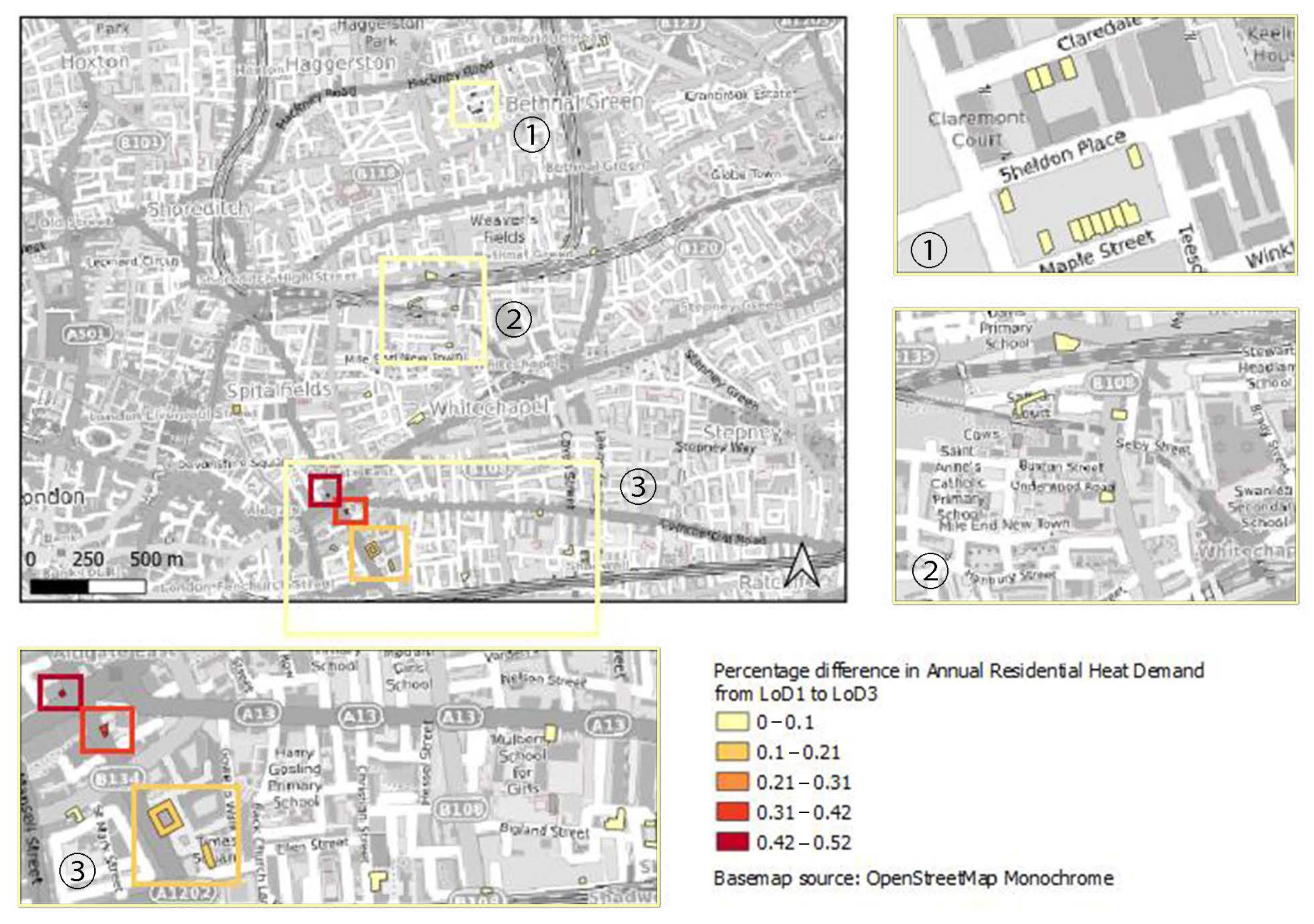
4.1.4. Percentage Difference in Annual Residential Heat Demand—Case Study Area 1
4.1.5. Percentage Difference in Annual Residential Heat Demand—Case Study Area 2
4.2. Adaptive Comfort Level
4.2.1. Annual Comfort Levels—Case Study Area 1
4.2.2. Annual Comfort Levels—Case Study Area 2
5. Discussion
5.1. Annual Residential Heat Demand and LoDs
5.2. Annual Residential Heat Demand and Comfort Level
6. Conclusions
Author Contributions
Funding
Institutional Review Board Statement
Informed Consent Statement
Data Availability Statement
Conflicts of Interest
References
- Yao, S. Building Integration of Sustainable Energy Technologies on a Detached House in Shanghai; Center on Global Energy Policy at Columbia University: New York, NY, USA, 2019; p. 77. Available online: https://www.energypolicy.columbia.edu/publications/energy-and-development-changing-world-framework-21st-century/ (accessed on 20 April 2023).
- Omer, M. Energy use and environmental impacts: A general review. J. Renew. Sustain. Energy 2009, 1, 053101. [Google Scholar] [CrossRef]
- Ismail, F.H.; Shahrestani, M.; Vahdati, M.; Boyd, P.; Donyavi, S. Climate change and the energy performance of buildings in the future—A case study for prefabricated buildings in the UK. J. Build. Eng. 2021, 39, 102285. [Google Scholar] [CrossRef]
- Pachauri, R.K.; Allen, M.R.; Barros, V.R.; Broome, J.; Cramer, W.; Christ, R.; Church, J.A.; Clarke, L.; Dahe, Q.; Dasgupta, P.; et al. Climate Change 2014: Synthesis Report. Contribution of Working Groups I, II and III to the Fifth Assessment Report of the Intergovernmental Panel on Climate Change; IPCC: Geneva, Switzerland, 2014; p. 151. Available online: https://epic.awi.de/id/eprint/37530/1/IPCC_AR5_SYR_Final.pdf (accessed on 9 April 2021).
- UN. UN Survey. More Than Half of World’s Population Now Living in Urban Areas, UN Survey Finds. UN News. 2014. Available online: https://news.un.org/en/story/2014/07/472752-more-half-worlds-population-now-living-urban-areas-un-survey-finds (accessed on 9 April 2021).
- Wang, S.; Fang, C.; Guan, X.; Pang, B.; Ma, H. Urbanisation, energy consumption, and carbon dioxide emissions in China: A panel data analysis of China’s provinces. Appl. Energy 2014, 136, 738–749. [Google Scholar] [CrossRef]
- Biljecki, F. The Concept of Level of Detail in 3D City Models; GISt Report No. 62; Delft University of Technology: Delft, The Netherlands, 2013; p. 70. [Google Scholar]
- Agugiaro, G.; Hauer, S.; Nadler, F. Coupling of CityGML-based semantic city Models with energy simulation tools: Some experiences. In Proceedings of the 20th International Conference on Urban Planning, Regional Development and Information Society, Ghent, Belgium, 5–7 May 2015. [Google Scholar]
- Trace Software. The Level of Detail and the Level of Development in the BIM Environment. 2019. Available online: https://www.trace-software.com/blog/the-level-of-detail-and-the-level-of-development-in-the-bim-environment/ (accessed on 12 June 2021).
- Tian, W. A review of sensitivity analysis methods in building energy analysis. Renew. Sustain. Energy Rev. 2013, 20, 411–419. [Google Scholar] [CrossRef]
- De Wilde, P.; Tian, W. Preliminary application of a methodology for risk assessment of thermal failures in buildings subject to climate change. In Proceedings of the Eleventh International IBPSA Conference, Glasgow, Scotland, 27–30 July 2009. [Google Scholar]
- Tian, W.; de Wilde, P. Uncertainty and sensitivity analysis of building performance using probabilistic climate projections: A UK case study. Autom. Constr. 2011, 20, 1096–1109. [Google Scholar] [CrossRef]
- Gustafsson, S.-I. Sensitivity analysis of building energy retrofits. Appl. Energy 1998, 61, 11. [Google Scholar] [CrossRef]
- Hygh, J.S.; DeCarolis, J.F.; Hill, D.B.; Ranjithan, S.R. Multivariate regression as an energy assessment tool in early building design. Build. Environ. 2012, 57, 165–175. [Google Scholar] [CrossRef]
- Hopfe, J.; Hensen, J.L.M. Uncertainty analysis in building performance simulation for design support. Energy Build. 2011, 43, 2798–2805. [Google Scholar] [CrossRef]
- Ioannou, A.; Itard, L. Energy performance and comfort in residential buildings: Sensitivity for building parameters and occupancy. Energy Build. 2015, 92, 216–233. [Google Scholar] [CrossRef]
- Olivero, E.; Onillon, E.; Beguery, P.; Brunet, R.; Marat, S.; Azar, M. On key parameters influencing building energy performance. In Proceedings of the Building Simulation 2015: 14th Conference of IBPSA, Hyderabad, India, 7–9 December 2015; p. 10. [Google Scholar]
- Zhang, A.; Bokel, R.; Van den Dobbelsteen, A.; Sun, Y.; Huang, Q.; Zhang, Q. The effect of geometry parameters on energy and thermal performance of school buildings in cold climates of China. Sustainability 2017, 9, 20. [Google Scholar] [CrossRef]
- Parasonis, J.; Keizikas, A. Possibilities to reduce the energy demand for multistory residential buildings. In Proceedings of the 10th International Conference “Modern Building Materials, Structures and Techniques”, Vilnius, Lithuania, 19–21 May 2010; p. 5. [Google Scholar]
- Hemsath, T.L. Building design with energy performance as primary agent. Energy Procedia 2015, 78, 6. [Google Scholar] [CrossRef]
- Ghiai, M.M.; Mahdavinia, M.; Parvane, F.; Jafarikhah, S. Relation between energy consumption and window to wall ratio in high-rise office buildings in Tehran. Eur. Online J. Nat. Soc. Sci. 2014, 3, 10. [Google Scholar]
- Robinson, D.; Haldi, F.; Leroux, P.; Perez, D.; Rasheed, A.; Wilke, U. CitySim: Comprehensive micro-simulation of resource flows for sustainable urban planning. In Proceedings of the Eleventh International IBPSA Conference, Glasgow, Scotland, 27–30 July 2009. [Google Scholar]
- Frayssinet, L.; Merlier, L.; Kuznik, F.; Hubert, J.-L.; Milliez, M.; Roux, J.-J. Modeling the heating and cooling energy demand of urban buildings at city scale. Renew. Sustain. Energy Rev. 2018, 81, 2318–2327. [Google Scholar] [CrossRef]
- APUR. Consommations D’énergie et Émission de Gaz à Effet’. 2007. Available online: https://www.apur.org/fr/nos-travaux/consommations-energie-emissions-gaz-effet-serre-liees-chauffage-residences-principales-parisiennes (accessed on 2 February 2023).
- Rosser, J.F.; Boyd, D.S.; Long, G.; Zakhary, S.; Mao, Y.; Robinson, D. Predicting residential building age from map data. Comput. Environ. Urban Syst. 2019, 73, 56–67. [Google Scholar] [CrossRef]
- Kaden, R.; Kolbe, T.H. City-wide total energy demand estimation of buildings using semantic 3D city models and statistical data. ISPRS Ann. Photogramm. Remote Sens. Spatial Inf. Sci. 2013, II-2/W1, 163–171. [Google Scholar] [CrossRef]
- Strzalka, A.; Bogdahn, J.; Coors, V.; Eicker, U. 3D City modeling for urban scale heating energy demand forecasting. HVAC&R Res. 2011, 17, 15. [Google Scholar]
- Dochev, I. Computing Residential Heat Demand in Urban Space using QGIS. A Case Study for Shumen, Bulgaria. 2016. Available online: http://programm.corp.at/cdrom2016/files/CORP2016_proceedings.pdf (accessed on 14 April 2021).
- ‘TABULA WebTool’. Available online: https://webtool.building-typology.eu/#bm (accessed on 25 June 2021).
- Nicol, F. Thermal Comfort: A Handbook for Field Studies Towards an Adaptive Model; University of East London: London, UK, 1993. [Google Scholar]
- Taleghani, M.; Tenpierik, M.; Kurvers, S.; van den Dobbelsteen, A. A review into thermal comfort in buildings. Renew. Sustain. Energy Rev. 2013, 26, 201–215. [Google Scholar] [CrossRef]
- Frontczak, M.; Wargocki, P. Literature survey on how different factors influence human comfort in indoor environments. Build. Environ. 2011, 46, 922–937. [Google Scholar] [CrossRef]
- De Dear, R.; Brager, G.S. Developing an Adaptive Model of Thermal Comfort and Preference. 1998. Available online: https://escholarship.org/uc/item/4qq2p9c6 (accessed on 8 March 2023).
- Yang, X.; Hu, M.; Heeren, N.; Zhang, C.; Verhagen, T.; Tukker, A.; Steubing, B. A combined GIS-archetype approach to model residential space heating energy: A case study for the Netherlands including validation. Appl. Energy 2020, 280, 115953. [Google Scholar] [CrossRef]
- Nouvel, R.; Schulte, C.; Eicker, U.; Pietruschka, D.; Coors, V. CityGML-based 3D city model for energy diagnostics and urban energy policy support. IBPSA World 2013, 2013, 9. [Google Scholar]
- Coulter, T.L.S.; Leicht, R.M. A sensitivity analysis of energy modeling input parameters for energy retrofit projects. In Proceedings of the Construction Research Congress 2014, Atlanta, GE, USA, 19–21 May 2014; pp. 2244–2254. [Google Scholar] [CrossRef]
- Ratti, C.; Baker, N.; Steemers, K. Energy consumption and urban texture. Energy Build. 2005, 37, 762–776. [Google Scholar] [CrossRef]
- Baker, F.; Smith, C. A GIS and object based image analysis approach to mapping the greenspace composition of domestic gardens in Leicester, UK. Landsc. Urban Plan. 2019, 183, 133–146. [Google Scholar] [CrossRef]
- ‘Colouring London’. Available online: https://colouring.london (accessed on 26 June 2021).
- Digimap Ordnance Survey’. Available online: https://digimap.edina.ac.uk/os (accessed on 26 June 2021).
- Ordnance Survey MasterMap Building Height Attribute|OS Products’. Available online: https://www.ordnancesurvey.co.uk/business-government/products/mastermap-building (accessed on 20 June 2022).
- Centreforcities. Average Space per Resident. 2018. Available online: https://www.centreforcities.org/reader/making-room/how-much-space-do-people-in-different-cities-have/ (accessed on 2 February 2023).
- Tabula, E. Building Typology Brochure England. 2014. Available online: https://episcope.eu/fileadmin/tabula/public/docs/brochure/GB_TABULA_TypologyBrochure_BRE.pdf (accessed on 2 February 2023).
- Public Health England. Minimum Home Temperature Thresholds for Health in Winter—A Systematic Literature Review; Public Health England: London, UK, 2014. [Google Scholar]
- Passivhaus Institut Passive House Planning Package (PHPP). Available online: https://passivehouse.com/04_phpp/04_phpp.htm (accessed on 4 March 2023).
- Urbano. Food4Rhino. 2019. Available online: https://www.food4rhino.com/en/app/urbano (accessed on 13 March 2023).
- ‘Ladybug Tools|Home Page’. Available online: https://www.ladybug.tools/ (accessed on 13 March 2023).
- ‘EnergyPlus’. Available online: https://energyplus.net/ (accessed on 13 March 2023).
- ‘Standard 55—Thermal Environmental Conditions for Human Occupancy’. Available online: https://www.ashrae.org/technical-resources/bookstore/standard-55-thermal-environmental-conditions-for-human-occupancy (accessed on 13 March 2023).
- GOV.UK. Live Tables on Energy Performance of Buildings Certificates. 2021. Available online: https://www.gov.uk/government/statistical-data-sets/live-tables-on-energy-performance-of-buildings-certificates (accessed on 10 August 2021).


| LoD1 | LoD2 | LoD3 | Mean-LoDs | GOV.UK | |
|---|---|---|---|---|---|
| Energy demand kWh/(m2·a) | 313.84 | 314.58 | 312.99 | 313.80 | 273.45 |
| Difference with GOV.UK | 40.39 | 41.13 | 39.54 | 40.35 |
| Building ID | Annual Heat Demand (kWh/m2) | Comfort Conditions Mean | Thermal Comfort Percentage Mean (%) |
|---|---|---|---|
| 2078778 | 205.13 | −0.82 | 15.44 |
| 1983230 | 355.64 | −0.83 | 13.19 |
| 2076468 | 377.24 | −0.46 | 93.73 |
| 1964588 | 380.93 | −0.46 | 90.88 |
| 2078781 | 386.97 | −0.54 | 97.55 |
| Building ID | Annual Heat Demand (kWh/m2) | Comfort Conditions Mean | Thermal Comfort Percentage (%) |
|---|---|---|---|
| 1961379 | 596.95 | −0.60 | 96.88 |
| 1961376 | 596.04 | −0.62 | 96.98 |
| 1983228 | 532.65 | −0.46 | 92.60 |
| 2078602 | 518.59 | −0.83 | 14.23 |
| 1948731 | 518.37 | −0.47 | 91.15 |
| Building ID | Annual Heat Demand (kWh/m2) | Comfort Conditions Mean | Thermal Comfort Percentage (%) |
|---|---|---|---|
| 1045310 | 69.97 | −0.23 | 95.84 |
| 77905 | 72.54 | −0.27 | 89.43 |
| 1053318 | 72.57 | −0.82 | 16.38 |
| 1382107 | 74.39 | −0.82 | 16.33 |
| 1002073 | 74.43 | 0.04 | 96.01 |
| Building ID | Annual Heat Demand (kWh/m2) | Comfort Conditions Mean | Thermal Comfort Percentage (%) |
|---|---|---|---|
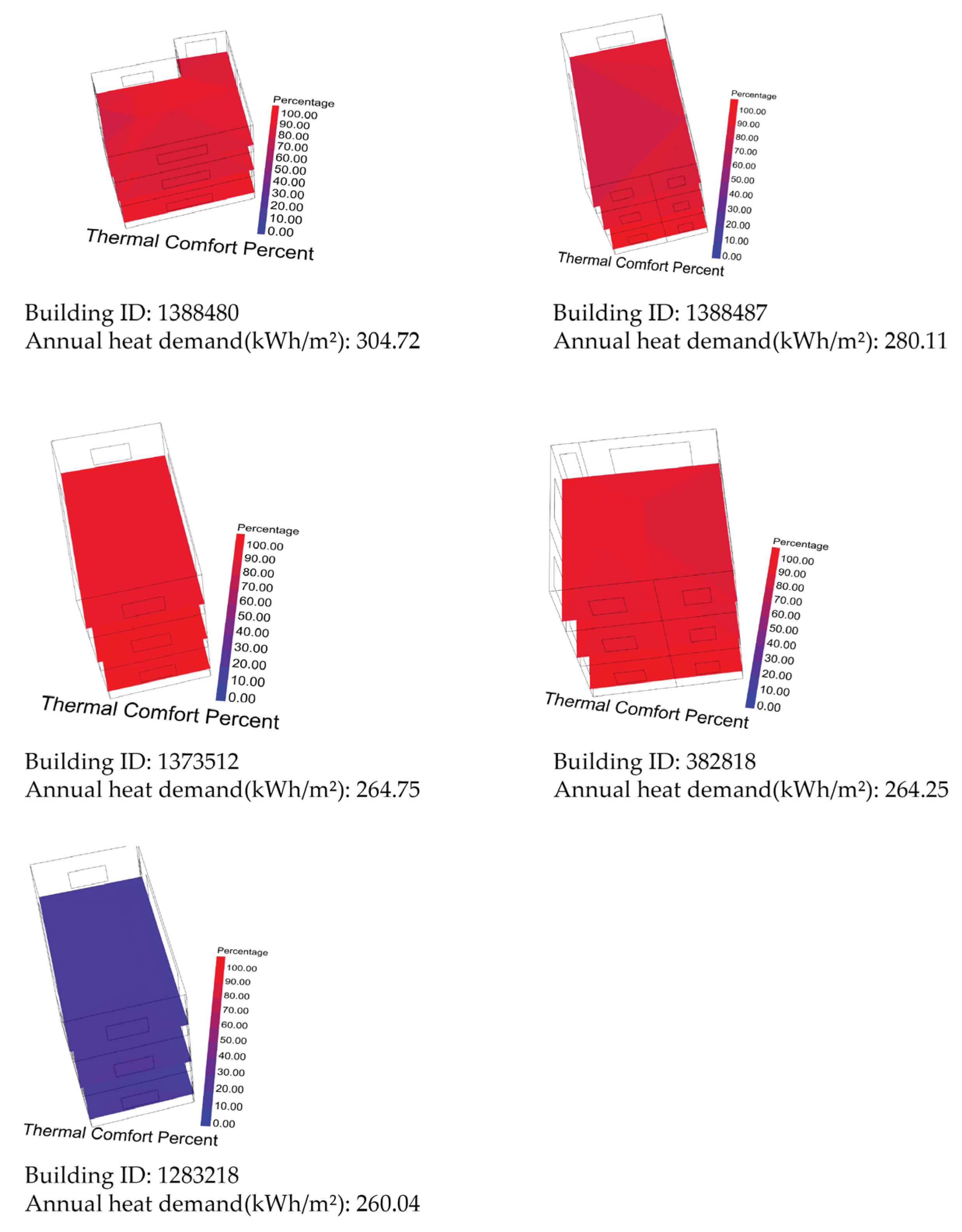
| 1388480 | 304.72 | −0.40 | 86.98 |
| 1388487 | 280.11 | −0.43 | 87.14 |
| 1373512 | 264.75 | −0.52 | 94.88 |
| 382818 | 264.25 | −0.46 | 91.80 |
| 1283218 | 260.04 | −0.84 | 12.94 |
Disclaimer/Publisher’s Note: The statements, opinions and data contained in all publications are solely those of the individual author(s) and contributor(s) and not of MDPI and/or the editor(s). MDPI and/or the editor(s) disclaim responsibility for any injury to people or property resulting from any ideas, methods, instructions or products referred to in the content. |
© 2023 by the authors. Licensee MDPI, Basel, Switzerland. This article is an open access article distributed under the terms and conditions of the Creative Commons Attribution (CC BY) license (https://creativecommons.org/licenses/by/4.0/).
Share and Cite
Apostolopoulou, A.; Zhu, M.; Jin, J. Parametric Assessment of Building Heating Demand for Different Levels of Details and User Comfort Levels: A Case Study in London, UK. Sustainability 2023, 15, 8374. https://doi.org/10.3390/su15108374
Apostolopoulou A, Zhu M, Jin J. Parametric Assessment of Building Heating Demand for Different Levels of Details and User Comfort Levels: A Case Study in London, UK. Sustainability. 2023; 15(10):8374. https://doi.org/10.3390/su15108374
Chicago/Turabian StyleApostolopoulou, Athanasia, Mingyu Zhu, and Jiayi Jin. 2023. "Parametric Assessment of Building Heating Demand for Different Levels of Details and User Comfort Levels: A Case Study in London, UK" Sustainability 15, no. 10: 8374. https://doi.org/10.3390/su15108374
APA StyleApostolopoulou, A., Zhu, M., & Jin, J. (2023). Parametric Assessment of Building Heating Demand for Different Levels of Details and User Comfort Levels: A Case Study in London, UK. Sustainability, 15(10), 8374. https://doi.org/10.3390/su15108374