Economic Growing Quantity Model with Mortality in Newborn Items and Inhibition Cost of Ammonia Production under All-Units Discount Policy

Abstract

The amount of global ammonia (NH₃) emissions is growing continuously, similar to the damage to the environment, particularly humans and animals, caused by those emissions. Various problems derived from pollution by ammonia emissions have attracted increasing attention in recent years. In particular, accumulation of ammonia in poultry farms is a concern for the poultry industry as it can lead to possible damage due to reduced bird performance, damage to the respiratory tract and skin of birds, and thus loss of customers. As birds age, ammonia production increases due to factors such as feeding and mobility, requiring the application of solutions to reduce it such as the use of fans, feed supplements, and temperature adjustments to improve bird health. These solutions impose additional costs on poultry farms to combat ammonia emissions. This study presents a general economic growing quantity (EGQ) model that includes the cost of inhibition of ammonia production during the growing period. In addition, the model is formulated under an all-units discount policy, where the price of newborn items is related to the size of the order purchased from the supplier. Furthermore, the model assumed that some newborn items are dead when the lot is received because of stress experiences and incidents during the catching, loading, transportation, and unloading. Finally, two versions of the proposed general EGQ model are presented: EGQ with no discount and EGQ with known slaughter age.

1. Introduction

The analysis of inventory problems for growing items is a new and significant topic in the inventory management literature. The model of economic order quantity (EOQ) for growing items or economic growing quantity (EGQ) was first presented by Rezaei [1]. EGQ models do not consider the common assumption of lot size problems, in which the weight of the items remains constant until consumption, while the former models assume that the weight increases after the items are received. EGQ models are common and usable in inventory systems such as livestock, poultry, and fish farming. In these cases, a company purchases several newborn animals, such as chicks, calves, or lambs from suppliers, and upon receipt, the farm raises them until they reach proper slaughter weight. The EGQ model balances the amount of the initial order for newborn items and the age of slaughter to maximize profit. The model considers the items’ growth function that shows the relationship between their weight and age. Therefore, the weight of the items is considered, instead of the number of items, in the EGQ model inventory graph.

Zhang et al. [2] presented a second paper on lot sizing problems for growing items in 2016. They considered one of the important aspects of environmental effects for companies, as they modeled a government-imposed carbon production tax over the growth period of the items. Therefore, they added this tax to the total inventory cost and obtained the optimal order quantity and the optimal slaughter age. Carbon emissions that occur from animal meat production are primarily associated with manure emissions and the production of feed for livestock and poultry. Due to these factors, the government sets a tax that emitters must pay for carbon production. Next, De-la-Cruz-Márquez et al. [3] developed an EGQ model with shortage and price-dependent demand, based on the model presented by Zhang et al. [2]. Additionally, Rana et al. [4] proposed an EGQ model for the effects of carbon emissions with a deteriorating process under a permissible delay policy. Concurrently, Gharaei and Almehdawe [5] addressed the impacts of carbon emissions emitted from produced manure, fermentation processes, and transportation in an EGQ model.

Nobil et al. [6] developed an EGQ model considering the admissibility of deficiency. An innovation in their work is the use of a linear approximation function for the growth function, which made the optimal solution easily derived in a few simple steps. After that, Nobil and Taleizadeh [7] presented a practical and realistic mode for mathematical modeling of the EGQ problems. When ordering newborn animals, it must be ensured that the quantity ordered is discrete; therefore, in their model, the corresponding decision variable is modeled as a discrete number.

A common assumption in the EGQ models has been to consider an inventory system for raising only one growing type of animal, until Khalilpourazari and Pasandideh [8] presented an EGQ model for an inventory system with multiple growing items. They assumed that several types of newborn animals could be bought and bred. Additionally, they integrated other assumptions such as storage capacity, budget in hand, and the maximum allowed cost of breeding and maintenance. Finally, the model, due to its structural complexity, was solved with two new meta-heuristic algorithms named the sine cosine crow search algorithm and the water cycle moth–flame optimization algorithm. The vast majority of EGQ models have focused on the farmer level, but Malekitabar et al. [9] considered two levels: farmer and supplier. The supplier raises newborn rainbow trout and then sells them to the farmer. Subsequently, the fish farmer grows the rainbow trout until they reach maturity and slaughter age, finally selling them to the market.

Recently, Gharaei and Almehdawe [10] applied the uniform distribution as the probability density function of survival and mortality over the growth period. Likewise, Sebatjane and Adetunji [11] proposed an EGQ model with the mortality function as a fraction of total items that do not survive the growing period. Another important extension to the EGQ models is the number of poor-quality items produced during the growing period that should be identified and removed. Sebatjane and Adetunji [12] extended the models of Rezaei [1] and Nobil et al. [6]. They considered an inspection time at the end of the breeding period, in which poor-quality items are identified and sold to the market at a lower price. In accordance with a sustainable green breeding policy, Nobil et al. [13] suggested an EGQ model with a practical polynomial function of CO₂ emissions, which is dependent both on the age of the animals and on the mortality function. The goal was to choose the best number of chicks to purchase from the supplier at the correct age for slaughter to save on overall costs. To increase the profits of livestock and poultry farms and reduce overall carbon emissions, Khan et al. [14] examined combined prepayment installment, pricing, and replenishment choices for a growing item under cap-and-price, cap-and-trade, and carbon tax legislation.

Under inventory policies, suppliers commonly recommend one of two forms of quantity discounts. The all-units quantity discount results in decreased procuring costs for the whole order if the quantity requested is above a precise quantity named the breakpoint. The incremental-units quantity discount results in decreased procuring cost that only applies to products purchased above the breakpoint. We found only one study in growing items that works with discount policies. Sebatjane and Adetunji [15] applied the incremental discount policy for the purchase of growing items, considering a price that depends on the order size.

The inclusion of the food supply chain echelons is another significant extension in the literature on growing items. Sebatjane and Adetunji [16] addressed an inventory-production problem for growing items in a supply chain with three levels: farming, processing, and retail. The farmer raises newborn animals and then sends them to a processor once the animals reach the slaughter age. The processing plant slaughters the animals and packages them at a specified rate. The processor sends a certain number of equally sized shipments of processed items to a retailer that meets the consumer’s demand. Sebatjane and Adetunji [17] presented an EGQ model for optimizing management decisions in a perishable food items supply chain that starts with farming operations in which live inventory products are raised and ends with the consumption of processed stock. The farming and consumption stages are linked by a processing stage during which livestock or poultry are processed into a consumable product. Consumer demand at the consumption stage is a function of the selling price and the freshness of the processed stock. The farming, processing, and consumption stages comprise the three-tier network model with the objective to maximize the joint supply chain profit. Later, Sebatjane and Adetunji [18] addressed an EGQ model for a three-level supply chain, including a farmer, a processor, and a retailer. They assumed that customer demand is dependent on the inventory level and the product expiration date. In addition, Pourmohammad-Zia et al. [19] evaluated the effects of marketing policies and perishable items in place for a two-echelon supply chain, including a supplier and a retailer. The model focuses on two scenarios: centralized and decentralized supply chain with a profit-sharing contract.

Pourmohammad-Zia et al. [20] also extended an EOQ model for growing items in a three-level supply chain (supplier, producer, and multiple retailers) by establishing a trade-off between cost-efficiency and market coverage. Lately, Sebatjane [21] suggested some inventory management techniques for a multi-level supply chain for perishable foods that includes components that are deteriorating and growing. His study assumed that the farming echelon, where young growing items are bred until they reach an age of maturity, is at the upstream end of the supply chain. The live inventory products are delivered to the processing echelon, which includes activities such as slaughtering, cutting, and packaging.

A summary of the major contributions made by scholars on these topics is presented in Table 1. According to our search, the effects of ammonia on an inventory system have not been considered in any of the past studies on inventory models. Wang et al. [22] reported that the emission of ammonia, which is a hazardous gas that exists in industry and agriculture, has gradually been identified as a major participant in the high levels of haze in many developing and developed countries. Based on the study of Koerkamp [23], absorption of surplus amino acids is mainly excreted as uric acid in poultry, while undigested protein is excreted through the feces. Microbial degradation of undigested protein and uric acid in broiler litters creates ammonia (NH₃) as a by-product. Additionally, excreted nitrogen (N) is associated with deteriorating litter quality, which exists in NH₃ content and contributes to the spread of hock and foot lesions in broilers. High NH₃ concentrations inside the broiler farms, and prolonged exposure to this volatile N compound, negatively impact the performance and health of birds (Miles et al. [24]), as well as the health of farmworkers and customers (Webb et al. [25]).

Wang et al. [26] stated that the deposition of ammonia in the environment can impact plant diversity and productivity, as well as the life cycle of aquatics. Additionally, based on the work of Brink et al. [27], NH₃ is a precursor for particulate matter that contributes to lower air quality. Strategies such as nutrition adaptations and ventilation are used in poultry farms to reduce NH₃ emissions. Although these strategies avoid emissions, they represent an extra cost for the farms. Therefore, this study presents a general EGQ model with an ammonia production inhibition cost during the breeding period.

Another innovative aspect of this study is the use of a discount policy when purchasing items from suppliers. None of the previous studies, except Sebatjane and Adetunji [15], considered the effects of discounts on inventory control decisions for growing items. Their model investigates the incremental discount policy on an EGQ model for a livestock farm. The proposed model considers the impact of an all-units discount policy on the EGQ problem and investigates the mortality for newborn items purchased from the supplier. Additionally, Yılmaz et al. [28] investigated that stress-causing incidents and practices during the catching, loading, transportation, and unloading may increase the mortality of birds. Hence, this study assumes that a percentage of the newborn items received from the supplier are dead. In summary, a general EGQ model with mortality in newborn items and an inhibition cost of NH₃ production under an all-units discount policy is presented. In addition, two specific cases are considered for the general model: EGQ with no discount and EGQ with known slaughter age.

Table 1. A summary of the major contributions made by some scholars in the literature of EGQs.

Paper	Year	Objective Function	Solution Method	Growth Curve	Dead Newborn Animals	NH3 Emission	Discount	Types of Items
Rezaei [1]	2014	PF	Analytical	BW				P
Zhang et al. [2]	2016	CF	Analytical	BW				P
Sebatjane and Adetunji [12]	2019	PF	Analytical	BW/LR				P
Sebatjane and Adetunji [15]	2019	CF	Analytical	BW			ID	L
Sebatjane and Adetunji [16]	2019	CF	Analytical	BW				L
Khalilpourazari and Pasandideh [8]	2019	PF	Meta-heuristic	BW				P
Malekitabar et al. [9]	2019	PF	Game theory	BW	*			F
Nobil et al. [6]	2019	CF	Analytical	LR				P
Nobil and Taleizadeh [7]	2019	CF	Closed form	LR				P
Sebatjane and Adetunji [17]	2020	PF	Analytical	BW				L
Gharaei and Almehdawe [10]	2020	CF	Closed form	LR				P
De-la-Cruz-Márquez et al. [29]	2021	PF	Analytical	BW				P
Gharaei and Almehdawe [5]	2021	CF	Meta-heuristic	BW				P
Pourmohammad-Zia et al. [19]	2021	PF	Analytical	BW				P
Pourmohammad-Zia et al. [20]	2021	PF	Game theory	BW				P
Rana et al. [4]	2021	CF	Analytical	BW				P
Sebatjane and Adetunji [19]	2021	PF	Analytical	BW				P
De-la-Cruz-Márquez et al. [3]	2022	PF	Analytical	BW				P
Sebatjane and Adetunji [11]	2022	CF	Analytical	BW				P
Sebatjane [21]	2022	CF	Analytical	BW				P
Nobil et al. [13]	2023	CF	Analytical	BW				P
Khan et al. [14]	2023	PF	Analytical	BW				P
This paper		CF	Analytical	BW	*	*	AD	P

PF: profit function, CF: cost function, BW: biological weight, LR: linear rate, AD: all-units, ID: incremental, P: poultry, L: livestock, F: fish. The “*” means that the research work includes the characteristic.

Table 1. A summary of the major contributions made by some scholars in the literature of EGQs.

Paper	Year	Objective Function	Solution Method	Growth Curve	Dead Newborn Animals	NH3 Emission	Discount	Types of Items
Rezaei [1]	2014	PF	Analytical	BW				P
Zhang et al. [2]	2016	CF	Analytical	BW				P
Sebatjane and Adetunji [12]	2019	PF	Analytical	BW/LR				P
Sebatjane and Adetunji [15]	2019	CF	Analytical	BW			ID	L
Sebatjane and Adetunji [16]	2019	CF	Analytical	BW				L
Khalilpourazari and Pasandideh [8]	2019	PF	Meta-heuristic	BW				P
Malekitabar et al. [9]	2019	PF	Game theory	BW	*			F
Nobil et al. [6]	2019	CF	Analytical	LR				P
Nobil and Taleizadeh [7]	2019	CF	Closed form	LR				P
Sebatjane and Adetunji [17]	2020	PF	Analytical	BW				L
Gharaei and Almehdawe [10]	2020	CF	Closed form	LR				P
De-la-Cruz-Márquez et al. [29]	2021	PF	Analytical	BW				P
Gharaei and Almehdawe [5]	2021	CF	Meta-heuristic	BW				P
Pourmohammad-Zia et al. [19]	2021	PF	Analytical	BW				P
Pourmohammad-Zia et al. [20]	2021	PF	Game theory	BW				P
Rana et al. [4]	2021	CF	Analytical	BW				P
Sebatjane and Adetunji [19]	2021	PF	Analytical	BW				P
De-la-Cruz-Márquez et al. [3]	2022	PF	Analytical	BW				P
Sebatjane and Adetunji [11]	2022	CF	Analytical	BW				P
Sebatjane [21]	2022	CF	Analytical	BW				P
Nobil et al. [13]	2023	CF	Analytical	BW				P
Khan et al. [14]	2023	PF	Analytical	BW				P
This paper		CF	Analytical	BW	*	*	AD	P

PF: profit function, CF: cost function, BW: biological weight, LR: linear rate, AD: all-units, ID: incremental, P: poultry, L: livestock, F: fish. The “*” means that the research work includes the characteristic.

The rest of this paper is organized as follows: The three proposed models are explained and formulated in Section 2. Next, Section 3 presents the solution procedures for each model, whereas Section 4 uses some numerical examples to validate the proposed algorithms. Finally, Section 5 presents some general conclusions and future research ideas.

2. Proposed Models

This section documents the proposed models, the notations, and the assumptions. Then, the mathematical formulation of the models (a) with no discount, (b) all-units discount, and (c) all-units discount with known slaughter age are explained by considering the nature of the growing items.

2.1. Notations and Assumptions

The indices of the time and discount categories based on a price are defined as $t=\mathrm{1,2},\dots$ and $i=\mathrm{1,2},\dots ,J$, respectively, and the rest of notation of the model is as follows:

• Parameters:

$J$: the number of discount categories based on a price; $i=\mathrm{1,2},\dots ,J$

$m_t$: the weight of a broiler at time $t$ (weight unit)

$E$: the highest length of breeding time (day)

$W$: the lowest length of the breeding time (day)

$D$: the rate of demand to weight unit (weight unit/year)

$\alpha$: the fraction of the purchased chicks from the supplier that are dead or of poor quality.

$r$: the holding cost percentage rate per year.

$u_i$: the weight volume breakpoint in units for a unit purchasing cost (weight unit)

$p_i$: the purchasing cost per weight unit for price range $i$ (monetary unit/weight unit) if $u_i\le y<u_{i+1}$

$S$: the setup cost per growing cycle (monetary unit/setup)

$x$: the cost of production (feeding) during growing period per unit item (monetary unit/unit item)

$z$: the inhibition cost of ammonia production (monetary unit/microliter/day·square meter·weight unit)

$f\left(t\right)$: the polynomial function of feeding consumption (unit items)

$v\left(t\right)$: the exponential function of ammonia production (microliter/day·square meter·bird).

$k$: the growth rate.

$A$: the asymptotic weight.

$b$: the integration constant of the growth function.

$n$: the shape parameter of the growth function.

$t_d$: the demand periods.

$Q$: the total weight at the slaughter time (weight unit).

$TCU$: the total cost per year (monetary unit).

${TCU}_i$: the total cost of breakpoint $i$ per year (monetary unit).

• Decision variables:

$y$: the total number of growth items ordered at the beginning of each cycle (unit items)

$t$: the slaughter age (day)

Figure 1 illustrates the weight stock level of broilers in the proposed model. In this inventory system, $y$ newborn chicks with an initial weight $m_0$ are purchased from the supplier. When the chicks are transported from the supplier to the poultry farm, a percentage of them (α) arrive dead. As a result, the number of live chicks that are available at the beginning of the period is equal to $\left(1-\alpha \right)y$. The poultry farm raises them for a period until they reach the ideal slaughter weight ($m_t$). At the time of slaughter ($t$), all broilers begin processed and shipped to the market for consumption, during the consumption period ($t_d$).

There are several works on live bird growth that define different growth functions. However, Richards in 1959 suggested one of the most important growth functions for live bird weight, which is named Richards’ function (Rezaei, [1]). This function is as follows:

$$m_t=A{\left(1+{be}^{-kt}\right)}^{\raisebox{1ex}{$1$}\!\left/ \!\raisebox{-1ex}{$n$}\right.}$$

(1)

where $m_t$ is the body weight of a live bird at age $t$.

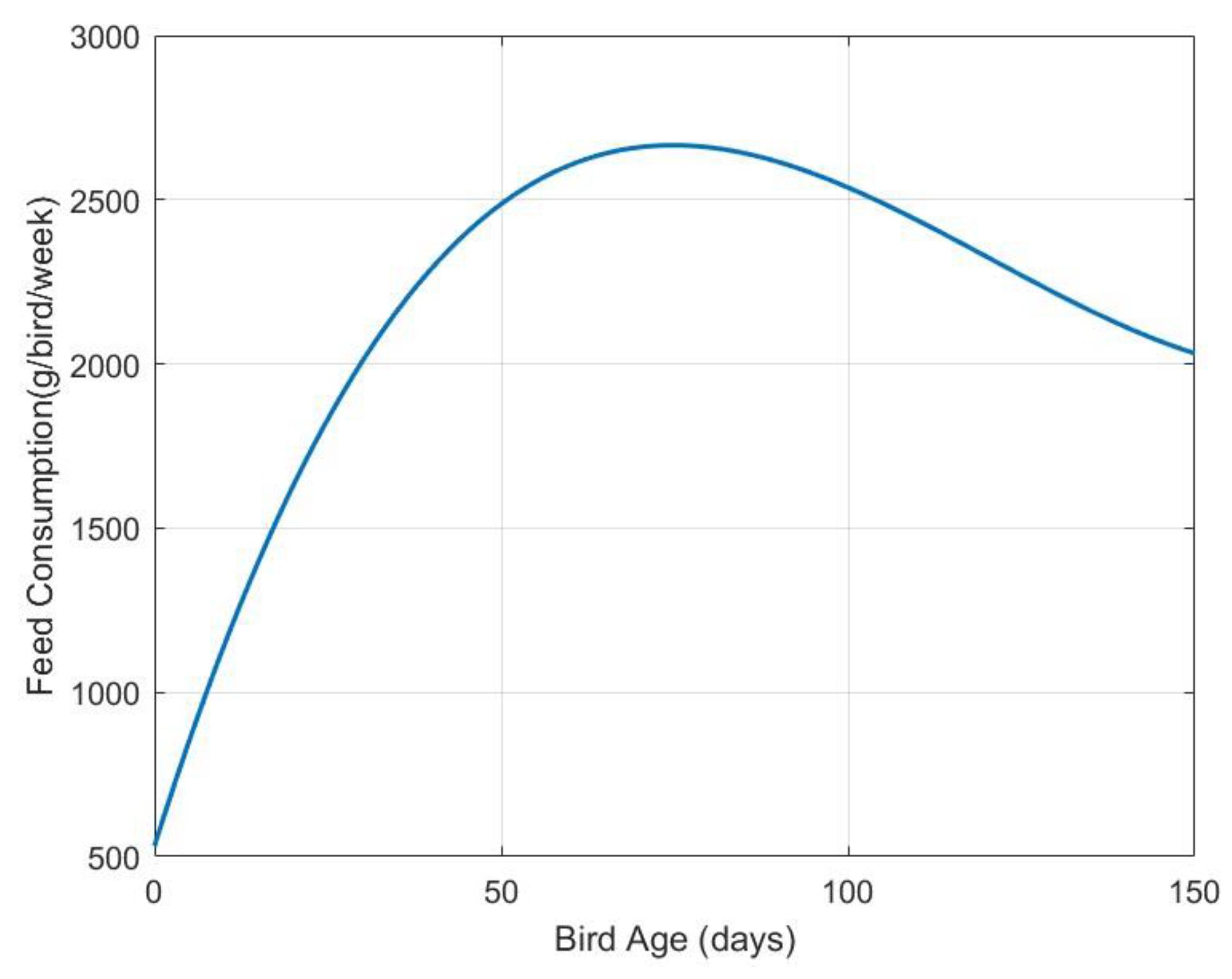
In the breeding period, birds grow and feed with a function that is proposed by Goliomytis et al. [30]. Their age is represented by a polynomial function. The function is as follows:

$$f\left(t\right)=a_0+a_{1}t+a_2{t}^2+a_3{t}^3$$

(2)

where $a_0$, $a_1$, $a_2$, and $a_3$ are fixed and known coefficients.

According to Shah et al. [31], the biological process of broiler litter, manure, and protein composition has an important outcome, NH_3, emissions in poultry farms. NH₃ has a harmful effect that jeopardizes the health of live birds. The ammonia production function based on the age of the birds is taken from the work of Leonard et al. [32]. This function is an exponential curve and is defined as:

$$v\left(t\right)={\theta }_0{e}^{{\theta }_{1}t}$$

(3)

where ${\theta }_0$ and ${\theta }_1$ are fixed and known coefficients.

2.2. EGQ with No Discount

Due to customer demand, the model considers that a poultry farm purchases newborn birds (raw material), grows them to meet market slaughter weight, and processes them. The farm needs to cover the total cost of the inventory system, which includes setup cost, purchasing cost, holding cost, feeding cost, and ammonia production inhibition cost.

The cycle begins with cleaning activities to start the breeding process. According to Figure 1, when time is zero, the number of newborn chicks ($y$) is received with initial weight ($m_0$) from the supplier, so the purchasing cost per growth cycle is equal to $py{m}_0$, where $p$ is the purchasing cost per weight unit without discount. Additionally, the length of the consumption period is $t_d$, while the average weight of the inventory during the consumption period is $\left(1-\alpha \right)y{m}_t/2$. The holding cost per cycle is $rp{t}_{d}y{m}_t/2$, where $rp$ is the annual inventory cost per weight unit with no discount. The feeding function per weight unit, described in Equation (2), depends on the age of the bird. It is noted that $x$ and $t$ are considered as the feeding cost per unit and the length of the breeding period, respectively. The total feeding cost per cycle is $x\left(1-\alpha \right)y{\int }_0^{t}f\left(t\right)dt$=$x\left(1-\alpha \right)y{\int }_0^t(a_0+a_{1}t+a_2{t}^2+a_3{t}^3)dt$.

Finally, there is a cost of dealing with ammonia production defined by $z\left(1-\alpha \right)y{\int }_0^t{b}_0{e}^{b_{1}t}dt$. Therefore, the total cost per cycle with no discount is as follows:

$$\begin{gathered} TC=S+py{m}_0+\frac{rp{t}_d\left(1-\alpha \right)y{m}_t}{2} \\ +x\left(1-\alpha \right)y{\int }_0^t(a_0+a_{1}t+a_2{t}^2+a_3{t}^3)dt \\ +z\left(1-\alpha \right)y{\int }_0^t{\theta }_0{e}^{{\theta }_{1}t}dt \end{gathered}$$

(4)

To meet the total cost function per year, $TC$ should be divided by $t_d=\left(1-\alpha \right)y{m}_t/D=\left(\left(1-\alpha \right)yA{\left(1+{be}^{-kt}\right)}^{\raisebox{1ex}{$1$}\!\left/ \!\raisebox{-1ex}{$n$}\right.}\right)/D$. This means that the total cost function per year without discount is:

$$\begin{gathered} TCU=\frac{DS}{\left(1-\alpha \right)yA{\left(1+{be}^{-kt}\right)}^{\raisebox{1ex}{$1$}\!\left/ \!\raisebox{-1ex}{$n$}\right.}}+\frac{Dp{m}_0}{\left(1-\alpha \right)A{\left(1+{be}^{-kt}\right)}^{\raisebox{1ex}{$1$}\!\left/ \!\raisebox{-1ex}{$n$}\right.}} \\ +\frac{rp\left(1-\alpha \right)yA{\left(1+{be}^{-kt}\right)}^{\raisebox{1ex}{$1$}\!\left/ \!\raisebox{-1ex}{$n$}\right.}}{2}+\frac{Dz{\theta }_0\left(e^{{\theta }_{1}t}-1\right)}{{\theta }_{1}A{\left(1+{be}^{-kt}\right)}^{\raisebox{1ex}{$1$}\!\left/ \!\raisebox{-1ex}{$n$}\right.}} \\ +\frac{Dx\left(a_{0}t+\frac{a_1{t}^2}{2}+\frac{a_2{t}^3}{3}+\frac{a_3{t}^4}{4}\right)}{A{\left(1+{be}^{-kt}\right)}^{\raisebox{1ex}{$1$}\!\left/ \!\raisebox{-1ex}{$n$}\right.}} \end{gathered}$$

(5)

where $y$ and $t$ are the decision variables.

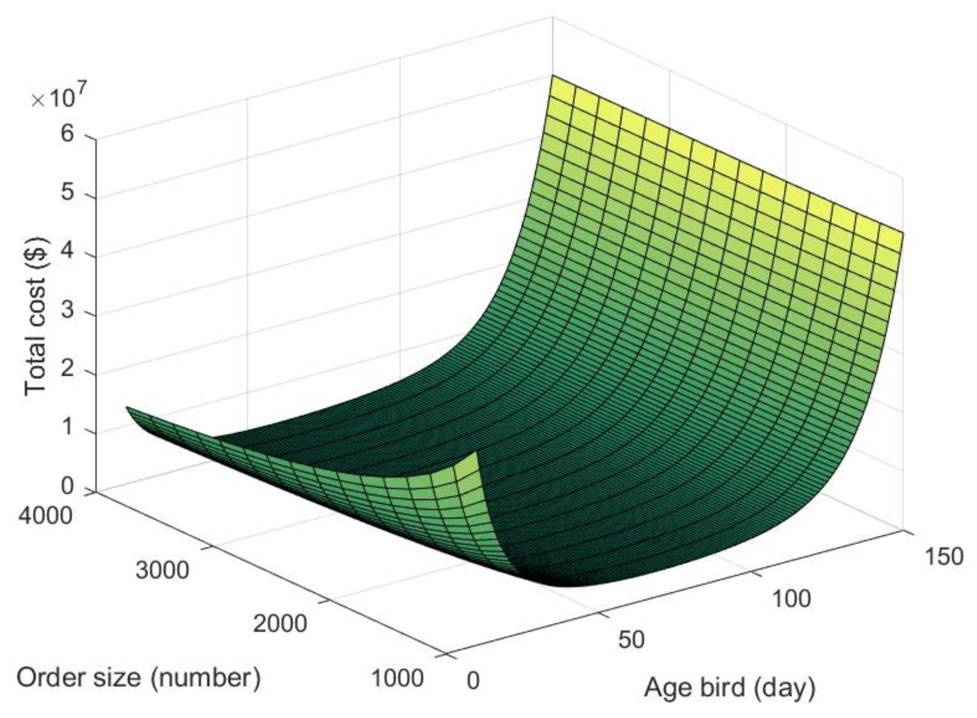
2.3. General EGQ

An EGQ model is considered in which the supplier offers an order quantity based on purchase cost per weight unit as given by:

$$p_i=\left\{\begin{array}{c}\begin{array}{cc}{p}_1& u_1\le y<u_2\end{array}\\ \begin{array}{l}\begin{array}{cc}{p}_2& u_2\le y<u_3\end{array}\\ \begin{array}{ll}⋮& ⋮\end{array}\\ \begin{array}{ll}{p}_J& u_J\le y\end{array}\end{array}\end{array}\right.$$

(6)

where $y$ is the order quantity, $u_1<u_2<\dots <u_J$ and $p_1>p_2>\dots >p_J$.

The total cost with an all-units discount is approximately equal to the case with no discount with only one difference: the purchasing and holding costs are changed with respect to the number of newborn birds that are ordered, as the acquisition price depends on the ordered quantity. Hence, the total cost function per year with an all-units discount (${TCU}_i$) is defined as follows:

$$\begin{gathered} {TCU}_i=\frac{DS}{\left(1-\alpha \right)yA{\left(1+{be}^{-kt}\right)}^{\raisebox{1ex}{$1$}\!\left/ \!\raisebox{-1ex}{$n$}\right.}}+\frac{D{p}_i{m}_0}{\left(1-\alpha \right)A{\left(1+{be}^{-kt}\right)}^{\raisebox{1ex}{$1$}\!\left/ \!\raisebox{-1ex}{$n$}\right.}} \\ +\frac{r{p}_i\left(1-\alpha \right)yA{\left(1+{be}^{-kt}\right)}^{\raisebox{1ex}{$1$}\!\left/ \!\raisebox{-1ex}{$n$}\right.}}{2}+\frac{Dz{\int }_0^t{\theta }_0{e}^{{\theta }_{1}t}dt}{A{\left(1+{be}^{-kt}\right)}^{\raisebox{1ex}{$1$}\!\left/ \!\raisebox{-1ex}{$n$}\right.}} \\ +\frac{Dx{\int }_0^t\left(a_0+a_{1}t+a_2{t}^2+a_3{t}^3\right)dt}{A{\left(1+{be}^{-kt}\right)}^{\raisebox{1ex}{$1$}\!\left/ \!\raisebox{-1ex}{$n$}\right.}};u_i\le y<u_{i+1} \end{gathered}$$

(7)

where $y$ and $t$ are the decision variables and the price ($p_i$) depends on the order size of $y$.

2.4. EGQ with Known Slaughter Age

This model assumes that the slaughter weight of chickens is known due to market behavior with respect to consumption weight through purchasing data. For example, in Asian countries such as Iran, this weight is 1.5 kg, in European countries such as the United Kingdom is about 2.2 kg and in the United States is about 3 kg (Nobil and Taleizadeh, [6]). As a result, once the consumption weight of broilers is known, the slaughter age is obtained according to the biological weight function Equation (1). Thus, slaughter age ($t$) can be considered as an input parameter and not as a decision variable. Therefore, the birds’ weight is easily computed using the slaughter age using Equation (1). In addition, the values of $f\left(t\right)$, and $v\left(t\right)$ are obtained by defining the slaughter age from Equations (2) and (3), respectively. Based on the value of $t$, the total cost in Equation (7) is adapted as follows:

$$\begin{gathered} T{CU}_i=\frac{DS}{\left(1-\alpha \right)y{m}_t}+\frac{r{p}_i\left(1-\alpha \right)y{m}_t}{2}+\frac{D{p}_i{m}_0}{\left(1-\alpha \right)m_t}+\frac{Dzv\left(t\right)}{m_t} \\ +\frac{Dxf\left(t\right)}{m_t};u_i\le y<u_{i+1} \end{gathered}$$

(8)

where $y$ is the only decision variable, and $p_i$ is a dependent variable.

3. Solution Procedures

In this section, the solution procedures of the three proposed models are shown. Due to the nature and assumptions of the models, each one has a specific procedure to obtain their optimal solution.

3.1. EGQ with No Discount

The decision variables used in this model are the slaughter age and the order size. Clearly, based on objective function (5), the purchasing cost is an input parameter with a constant value and does not depend on the order size. As the model is convex (see Appendix A), then the partial derivative of objective function (5) with respect to $t$ and $y$ are set equal to zero, as follows:

$$\begin{gathered} \frac{\partial TCU}{\partial t}=-\frac{DSk{be}^{-kt}}{Any\left(\alpha -1\right){\left(1+{be}^{-kt}\right)}^{\left(\raisebox{1ex}{$1$}\!\left/ \!\raisebox{-1ex}{$n$}\right.+1\right)}} \\ -\frac{Dp{m}_{0}k{be}^{-kt}}{An\left(\alpha -1\right){\left(1+{be}^{-kt}\right)}^{\left(\raisebox{1ex}{$1$}\!\left/ \!\raisebox{-1ex}{$n$}\right.+1\right)}} \\ +\frac{Akpry{be}^{-kt}\left(\alpha -1\right){\left(1+{be}^{-kt}\right)}^{\left(\raisebox{1ex}{$1$}\!\left/ \!\raisebox{-1ex}{$n$}\right.-1\right)}}{2n} \\ +\frac{Dz{\theta }_0{e}^{{\theta }_{1}t}}{A{\left(1+{be}^{-kt}\right)}^{\left(\raisebox{1ex}{$1$}\!\left/ \!\raisebox{-1ex}{$n$}\right.\right)}}+\frac{Dzbk{\theta }_0{e}^{-kt}\left(e^{{\theta }_{1}t}-1\right)}{An{\theta }_1{\left(1+{be}^{-kt}\right)}^{\left(\raisebox{1ex}{$1$}\!\left/ \!\raisebox{-1ex}{$n$}\right.+1\right)}} \\ +\frac{Dx\left(a_0+a_{1}t+a_2{t}^2+a_3{t}^3\right)}{A{\left(1+{be}^{-kt}\right)}^{\left(\raisebox{1ex}{$1$}\!\left/ \!\raisebox{-1ex}{$n$}\right.\right)}} \\ +\frac{Dxbk{e}^{-kt}\left(a_{0}t+\frac{a_1{t}^2}{2}+\frac{a_2{t}^3}{3}+\frac{a_3{t}^4}{4}\right)}{An{\left(1+{be}^{-kt}\right)}^{\left(\raisebox{1ex}{$1$}\!\left/ \!\raisebox{-1ex}{$n$}\right.+1\right)}}=0 \end{gathered}$$

(9)

$$\frac{\partial TCU}{\partial y}=-\frac{DS}{\left(1-\alpha \right)y^{2}A{\left(1+{be}^{-kt}\right)}^{\raisebox{1ex}{$1$}\!\left/ \!\raisebox{-1ex}{$n$}\right.}}+\frac{rp\left(1-\alpha \right)A{\left(1+{be}^{-kt}\right)}^{\raisebox{1ex}{$1$}\!\left/ \!\raisebox{-1ex}{$n$}\right.}}{2}=0$$

(10)

Based on Equation (10), the value of the order size is equal to:

$$y=\sqrt{\frac{2DS}{rp{\left(1-\alpha \right)}^2{A}^2{\left(1+{be}^{-kt}\right)}^{\raisebox{1ex}{$2$}\!\left/ \!\raisebox{-1ex}{$n$}\right.}}}$$

(11)

The optimal slaughter time cannot be obtained by a closed-form method from Equation (9), so a numerical method is used to solve it. Therefore, by substituting the order size value from Equation (11) into Equation (9), then the optimal slaughter age is obtained using the Newton–Raphson method by applying the following solution procedure:

• Step 1. Substituting the order size value of Equation (11) into Equation (9), solve for the value of $t$ from Equation (9) using the Newton–Raphson method.
• Step 2. Based on the value of $t^{*}$, compute the optimal value of $y^{*}$ using Equation (11).
• Step 3. Based on the value of $t^{*}$ and $y^{*}$, determine the optimal value of ${TCU}^{*}$ using Equation (5).

3.2. General EGQ

In this model, in addition to considering the slaughter age and the order size as decision variables, the purchasing cost is considered as not constant and as a dependent variable of the order size. This model is an extension of the EGQ model without discount. Like in the previous solution procedure, the partial derivatives of objective function (7) are set equal to zero as follows (see Appendix B to review the procedure to calculate the number of orders):

$$\begin{gathered} \frac{\partial {TCU}_i}{\partial t}=-\frac{DSk{be}^{-kt}}{Any\left(\alpha -1\right){\left(1+{be}^{-kt}\right)}^{\left(\raisebox{1ex}{$1$}\!\left/ \!\raisebox{-1ex}{$n$}\right.+1\right)}} \\ -\frac{D{p}_i{m}_{0}k{be}^{-kt}}{An\left(\alpha -1\right){\left(1+{be}^{-kt}\right)}^{\left(\raisebox{1ex}{$1$}\!\left/ \!\raisebox{-1ex}{$n$}\right.+1\right)}} \\ +\frac{Ak{p}_{i}ry{be}^{-kt}\left(\alpha -1\right){\left(1+{be}^{-kt}\right)}^{\left(\raisebox{1ex}{$1$}\!\left/ \!\raisebox{-1ex}{$n$}\right.-1\right)}}{2n} \\ +\frac{Dz{\theta }_0{e}^{{\theta }_{1}t}}{A{\left(1+{be}^{-kt}\right)}^{\left(\raisebox{1ex}{$1$}\!\left/ \!\raisebox{-1ex}{$n$}\right.\right)}}+\frac{Dzbk{\theta }_0{e}^{-kt}\left(e^{{\theta }_{1}t}-1\right)}{An{\theta }_1{\left(1+{be}^{-kt}\right)}^{\left(\raisebox{1ex}{$1$}\!\left/ \!\raisebox{-1ex}{$n$}\right.+1\right)}} \\ +\frac{Dx\left(a_0+a_{1}t+a_2{t}^2+a_3{t}^3\right)}{A{\left(1+{be}^{-kt}\right)}^{\left(\raisebox{1ex}{$1$}\!\left/ \!\raisebox{-1ex}{$n$}\right.\right)}} \\ +\frac{Dxbk{e}^{-kt}\left(a_{0}t+\frac{a_1{t}^2}{2}+\frac{a_2{t}^3}{3}+\frac{a_3{t}^4}{4}\right)}{An{\left(1+{be}^{-kt}\right)}^{\left(\raisebox{1ex}{$1$}\!\left/ \!\raisebox{-1ex}{$n$}\right.+1\right)}}=0 \end{gathered}$$

(12)

$$\frac{\partial {TCU}_i}{\partial y}=0\to y=\sqrt{\frac{2DS}{r{p}_i{\left(1-\alpha \right)}^2{A}^2{\left(1+{be}^{-kt}\right)}^{\raisebox{1ex}{$-2$}\!\left/ \!\raisebox{-1ex}{$n$}\right.}}}$$

(13)

By substituting the order size from Equation (13) into Equation (12), the optimal slaughter age can be obtained by the Newton–Raphson method. It is necessary to remark that $t_i$, $y_i^t$, and ${TCU}_i^t$ are the slaughter age, the order size, and the total cost at the breakpoint $i$($u_i\le y_i^t<u_{i+1}$), respectively. Therefore, the steps of the proposed solution procedure are as follows:

• Step 1. For $i=\mathrm{1,2}\dots J$

  (a)

  Substituting the value of Equation (13) into Equation (12), find the value of $t_i$ from Equation (12) using the Newton–Raphson method.

  (b)

  Based on the value of $t_i^{*}$, compute the value of $y_i$ using Equation (13).

  (c)

  If $u_i>y_i$, then $y_i^{*}=u_i$, else if $u_{i+1}<y_i$, then $y_i^{*}=u_{i+1}-1$, and hence go to Step 1 (d). Otherwise, $y_i^{*}=y_i$ ($u_i\le y_i<u_{i+1}$), then go to Step 1 (e).

  (d)

  Based on the value of $y_i$, find the value of $t_i$ from Equation (12) using the Newton–Raphson method

  (e)

  Having $t_i^{*}$ and $y_i^{*}$, obtain ${TCU}_i^{*}$ from Equation (7)

• Step 2. Compare the total cost (${TCU}_i^{*}$) of the solutions ($t_i^{*}$, $y_i^{*}$) for $i=\mathrm{1,2}\dots J$. The pair ($t_i^{*}$, $y_i^{*}$) that gives the lowest cost is the optimal solution for the problem.

3.3. EGQ with Known Slaughter Age

As stated before, the slaughter age is defined by market behavior and customer purchase data. Therefore, this model has only one decision variable, which is the order size ($y$). Now, the optimal order size is obtained by setting the derivation of objective function (8) regarding $y_i$ equal to zero, as follows:

$$\frac{\partial {TCU}_i}{\partial y}=-\frac{DS}{\left(1-\alpha \right)y^2{m}_t}+\frac{r{p}_i\left(1-\alpha \right)m_t}{2}=0$$

(14)

Therefore, the solution is:

$$y=\sqrt{\frac{2DS}{r{p}_i{\left(1-\alpha \right)}^2{m_t}^2}}$$

(15)

According to Equation (15), the order size value is like the classic EOQ model with all-units discount. Based on the classic EOQ, the solution procedure is as follows:

• Step 1. Define the slaughter age and compute the values of $m_t$, $f\left(t\right)$, and $v\left(t\right)$ by using Equations (1)–(3), respectively.
• Step 2. Set $i=J$
• Step 3. Determine the optimal value of the breakpoint $i$ ($y_i$) using Equation (15)
• Step 4. If $u_j>y_i$, then $y_i^{*}=u_j$ and go to Step 5. Otherwise, $y_i^{*}=y_i$; then, go to Step 6.
• Step 5. Set $i=i-1$ and go to Step 3
• Step 6. Obtain the optimal value of ${TCU}_i^{*}$ form Equation (8) according to all the $y_i^{*}$s obtained.
• Step 7. Compare the total cost (${TCU}_i^{*}$) of the optimal solution ($y_i^{*}$) for every breakpoint ($J,J-1,\dots .i$). The $y_i^{*}$ that provides the lowest cost is the optimal solution for the problem.

4. Numerical Examples

As is clear from the previous descriptions, the model with the all-units discount is a more comprehensive and complete model than the model without the discount, and its solutions will always be better or equal to the case without the discount. Additionally, the last model, which has a general discount and a specific slaughter age, is a special case of the model with a general discount, in which the slaughter time is known in advance based on market needs and customer requests. To demonstrate the application of the solution procedures for the three proposed models, a general numerical instance for a particular type of broiler inventory system is developed in this section. The general instance has been considered for all models; however, some parameters may change in each model. Based on the report of the European Food Safety Authority [33], farms can slaughter broilers from 21 days up to 150 days old. The usual slaughter age is 47 days in the US, while the slaughter age is 42 days in European countries. Therefore, the values of the minimum ($O$) and maximum ($W$) allowable length of breeding period are set equal to 21 and 55 respectively. The numerical instance uses the parameters of Richard’s growth curve and the feed consumption curve that are estimated by Goliomytis et al. [30], as follows:

$k=0.036;n=0.0087;A=6870.2;b=-0.043$, and

$a_0=532.2;a_1=67.15;a_2=-0.651;a_3=0.0018$.

Accordingly, the growth curve and the feed consumption curve applied for this instance are as follows (see Figure 2 and Figure 3):

$m_t=6870.2{\left(1+{0.043e}^{-0.036t}\right)}^{\raisebox{1ex}{$-1$}\!\left/ \!\raisebox{-1ex}{$0.0087$}\right.}$; and

$f\left(t\right)=532.2+67.15t-0.651t^2+0.0018t^3$.

Moreover, the exponential function $v\left(t\right)$ for NH₃ production (Microliter/day·m²·bird) is based on the work of Leonard et al. [32] with $b_0=19.44$ and $b_1=0.078$. Thus, the ammonia production curve is $v\left(t\right)=19.44e^{0.078t}$ (see Figure 4). The rest of the parameters in the general instance are $D=\mathrm{1,000,000,000}\mathrm{g}$, $m_0=45\mathrm{g}$, $r=0.02/\mathrm{year}$, $x=0.0001\$/\mathrm{g}/\mathrm{day}$, $S=5.000\$/\mathrm{cycle}$, and $z=0.00001\$/\mathsf{\mu }\mathrm{L}/\mathrm{d}·{\mathrm{m}}^2·\mathrm{bird}$.

4.1. EGQ with No Discount

Based on the general model parameters given above, the purchasing cost per gram is $p=0.01\$/g$. The optimal solutions for the EGQ model with no discount are obtained with the Section 3.1 solution procedure. Applying the Newton–Raphson method, the optimal slaughter age is $t^{*}=53.26\cong 53$. Next, substituting $t^{*}$ into Equations (11) and (5), the optimal order size and total cost are determined as follows: $y^{*}\cong \mathrm{75,472}$ chicks, and ${TCU}^{*}\cong \mathrm{3,091,349}$ $.

4.2. General EGQ

The same conditions and parameters from the EGQ model with no discount are used for the general EGQ model, except for one difference: the supplier sells newborn chicks at different prices based on the quantity ordered. Thus, $p=(p_1,p_2,p_3,p_4)=\left(\mathrm{0.010,0.008,0.006,0.004}\right)\$/\mathrm{g}$ and $u=(u_1,u_2,u_3,u_4)=\left(\mathrm{0,50000,80000,100000}\right)\mathrm{g}$. Applying the proposed solution procedure explained in Section 3.2, the optimal solution for each breakpoint is as follows:

• First Point ($0\le y\le \mathrm{50,000}$): $t_1^{\mathrm{*}}\cong 53$, $y_1^{\mathrm{*}}\cong \mathrm{50,000}$; and ${TCU}_1^{\mathrm{*}}\cong \mathrm{3,095,060}$ $.
• Second Point ($\mathrm{50,000}\le y\le \mathrm{80,000}$): $t_2^{\mathrm{*}}\cong 53$, $y_2^{\mathrm{*}}\cong \mathrm{80,000}$; and ${TCU}_2^{\mathrm{*}}\cong \mathrm{3,056,307}$ $.
• Third Point ($\mathrm{80,000}\le y\le \mathrm{100,000}$): $t_3^{\mathrm{*}}\cong 52$, $y_3^{\mathrm{*}}\cong \mathrm{100,000}$; and ${TCU}_3^{\mathrm{*}}\cong \mathrm{3,020,000}$ $.
• Fourth Point ($y\ge \mathrm{100,000}$): $t_4^{\mathrm{*}}\cong 52$, $y_4^{\mathrm{*}}\cong \mathrm{122,605}$; and ${TCU}_4^{\mathrm{*}}\cong \mathrm{2,982,433}$ $.
• Breakpoint 4 produces the lowest total cost (${TCU}_4^{*}\cong \mathrm{2,982,433}$), so the optimal solutions are $t^{*}=$ 52 days, $y^{*}=\mathrm{122,605}$ chicks, and ${TCU}^{*}=\mathrm{2,982,433}$ $.

4.3. EGQ with Known Slaughter Age

The EGQ model conditions and parameters (Section 4.2) are applied for this last numerical example, just with one difference: the slaughter age is considered equal to 62 days. Now, the optimal solution is easily obtained as follows by applying the solution procedure detailed in Section 3.3:

• Step 1. Using Equations (1)–(3)

$m_t=3959$ g, $f\left(t\right)=2614.5$, and $v\left(t\right)=2265$.

• Step 2 to 3. Using Equation (15)

$u_4=0.004\to y_4=\mathrm{97,303}$;

$u_3=0.006\to y_3=\mathrm{79,448}$;

$u_2=0.008\to y_2=\mathrm{68,804}$;

• Step 4 to 5.

Since $y_4^{\mathrm{*}}<u_4$, then $y_4^{\mathrm{*}}=u_4=\mathrm{100,000}$.

Since $y_3^{\mathrm{*}}<u_3$, then $y_3^{\mathrm{*}}=u_3=\mathrm{80,000}$.

Since $u_2\le y_3^{*}<u_3$, so the value of $y_2^{*}$ is equal to $y_2=\mathrm{68,804}$.

It is not necessary to check the lower breakpoint ($i=1$) as the order size value is between its range.

• Step 6. Using Equation (8)

${TCU}_2^{\mathrm{*}}=\mathrm{3,114,003}$, ${TCU}_3^{\mathrm{*}}=\mathrm{3,083,876}$; and ${TCU}_4^{\mathrm{*}}=\mathrm{3,052,760}$.

• Step 7.

Since ${TCU}_4^{*}<{TCU}_3^{*}<{TCU}_2^{*}$, so the optimal total cost is equal to ${{TCU}^{*}=TCU}_4^{*}=\mathrm{3,052,760}$ $, and thus, the optimal order size is ${y^{*}=y}_4^{*}=\mathrm{100,000}$ chicks.

5. Conclusions

NH₃ in poultry is a crucial biological process effect of the protein, litter, and manure composition generated on farms. When ammonia gas is exposed to moisture, it reacts and forms a basic, corrosive solution named ammonium. This aqueous solution causes harm to broilers. NH₃ production increases as poultry ages, so managers must use methods to regulate the temperature, adjust the ventilation rate, and regulate diet and feed supplements to counteract it. These methods impose additional costs on poultry farm operations, which must be included in the inventory models. In addition, the process of shipping newborn chicks from suppliers to farms causes a percentage of deaths due to stressors and incidents such as catching, loading, transporting, and unloading. Therefore, a general EGQ model with mortality in newborn chicks and ammonia production inhibition cost under an all-units discount policy is presented in this study. In this general model, the poultry farm acquires newborn items at a discount price, which is lower than the wholesale price if the quantity ordered is above a breakpoint. The optimal solutions are obtained by using an analytical approach. Additionally, two special cases of the general model are formulated and explained based on their widespread use in the real world. The first model, EGQ with no discount, assumes that the supplier does not offer any discount policy. This condition is common in real life as some items are special or in limited supply, so the supplier does not offer any discount for them. This model is also solved using an analytical approach. In the last model, the consumption weight of poultry items is known in advance in most countries due to customer interest and pre-existing purchasing data. Once the consumption weight is set, the slaughter age is calculated according to a biological weight function. Therefore, the second case is an EGQ with known slaughter age. It is proved that this model has a solution like the one of a classic EOQ model with an all-units discount policy.

The proposed models can be extended (a) by using amelioration and deterioration rates, (b) by considering an expiration date in the consumption period, (c) by introducing a mortality rate during the breeding period, among others. Additionally, this research can be extended to other farm operations like livestock and fishery. Finally, it is possible to investigate the environmental effects of other harmful gases produced in livestock and poultry farms.