Article

Short-Term Subway Passenger Flow Prediction Based on Time Series Adaptive Decomposition and Multi-Model Combination (IVMD-SE-MSSA)

College of Mechanical Engineering, Guangxi University, Nanning 530004, China
*
Author to whom correspondence should be addressed.
Sustainability 2023, 15(10), 7949; https://doi.org/10.3390/su15107949
Submission received: 25 March 2023 / Revised: 15 April 2023 / Accepted: 10 May 2023 / Published: 12 May 2023
(This article belongs to the Special Issue Advances in Smart City and Intelligent Transportation Systems)

Abstract

:
The accurate forecasting of short-term subway passenger flow is beneficial for promoting operational efficiency and passenger satisfaction. However, the nonlinearity and nonstationarity of passenger flow time series bring challenges to short-term passenger flow prediction. To solve this challenge, a prediction model based on improved variational mode decomposition (IVMD) and multi-model combination is proposed. Firstly, the mixed-strategy improved sparrow search algorithm (MSSA) is used to adaptively determine the parameters of the VMD with envelope entropy as the fitness value. Then, IVMD is applied to decompose the original passenger flow time series into several sub-series adaptively. Meanwhile, the sample entropy is utilized to divide the sub-series into high-frequency and low-frequency components, and different models are established to predict the sub-series with different frequencies. Finally, the MSSA is employed to determine the weight coefficients of each sub-series to combine the prediction results of the sub-series and get the final passenger flow prediction results. To verify the prediction performance of the established model, passenger flow datasets from four different types of Nanning Metro stations were taken as examples for carrying out experiments. The experimental results showed that: (a) The proposed hybrid model for short-term passenger flow prediction is superior to several baseline models in terms of both prediction accuracy and versatility. (b) The proposed hybrid model is excellent in multi-step prediction. Taking station 1 as an example, the MAEs of the proposed model are 3.677, 5.7697, and 8.1881, respectively, which can provide technical support for subway operations management.

1. Introduction

Urban rail transit has developed rapidly in the twenty-first century. As a safe, convenient, and green transport tool, the subway is the preferred choice for most people to travel [1]. However, the increase in passenger demand often leads to congestion in subways. Passenger flow prediction plays a vital role in relieving congestion, especially short-term passenger flow prediction (STPFP) [2]. On the one hand, STPFP can assist station managers in organizing and guiding passengers, relieving congestion, and avoiding accidents. On the other hand, operators can draw up corresponding passenger flow control tactics and optimize train schedules to promote the operational efficiency of the subway systems. Moreover, it can also provide convenience for passengers. Therefore, it is of great significance to predict the short-term subway passenger flow by using the passenger flow data collected by the automatic fare collection (AFC) equipment.
Many methods have been utilized for STPFP, which can be generally divided into parametric models and non-parametric models [3]. The parametric models include the Kalman filtering model [4], grey prediction [5], history average [6], and autoregressive integrated moving average and its variant models [7,8]. The parametric models seek a linear mapping relation based on statistical principles that are suitable for predicting linear and stationary time series. This kind of method has a weak ability to learn nonlinear relations in passenger flow data, and the prediction error is remarkable. To improve prediction accuracy, researchers apply non-parametric models to STPFP, which are better than parametric models at capturing features in historical ridership data. The random forest model [9], support vector machine (SVM) [10], shallow neural networks [11], and the Bayesian method [12] are a few examples. Although the non-parametric methods can learn more nonlinear relationships of time series, the prediction performance of non-parametric methods relies too much on complicated artificial feature engineering. Recently, deep learning technologies based on deep neural networks have shown good performance without feature engineering. Some researchers have used them for STPFP, such as deep belief networks [13], recurrent neural networks (RNN) [
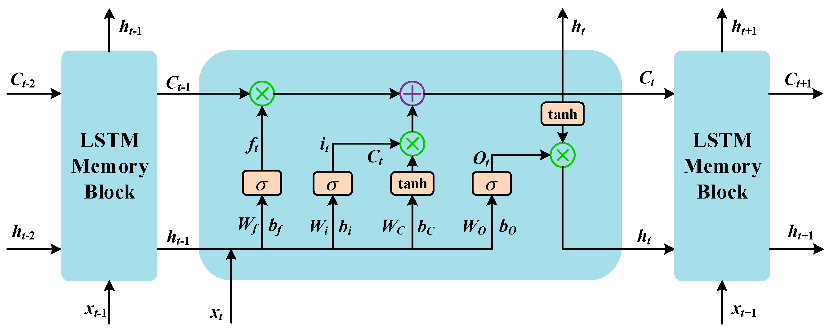
14], long short-term memory (LSTM) [15], convolutional neural networks [16], and graph convolutional neural networks [17]. Due to their strong generalization ability and big data training ability, deep learning models have become the mainstream model for STPFP.
However, in practice, the process of collecting subway passenger flow data is often interfered by many factors such as weather or emergencies, and there is a lot of noise in the original passenger flow data. This leads to the highly nonlinear and nonstationary nature of the passenger flow time series, which seriously affects the prediction performance of the models [18]. Recently, some data preprocessing techniques have been applied to passenger flow prediction. The idea is to reduce the influence of noise in the data through decomposition methods and improve the prediction accuracy of the model [19]. Wei et al. [3] used empirical mode decomposition (EMD) to decompose the subway passenger flow time series and proved that data preprocessing technology could significantly improve the prediction accuracy. Shen et al. [20] applied EMD to process volatility and nonlinear passenger flow data. Li et al. [21] conducted a secondary decomposition of bus passenger flow based on EMD to perform STPFP. Their experimental results showed that the model mixed with the data preprocessing method was a reliable and promising prediction method. Although the hybrid model based on EMD can significantly improve prediction accuracy, EMD has the disadvantage of mode mixing. Wu and Huang [22] proposed ensemble EMD (EEMD) based on adding Gaussian white noise to overcome the above shortcomings. Liu et al. [23] and Cao et al. [24] adopted the EEMD to decompose passenger flow and further indicated that the EEMD had better decomposition and denoising ability than the EMD. Although the prediction accuracy based on EEMD is better than that of EMD, the computational scale of EEMD is large, and there is residual noise. Yeh et al. [25] proposed a complementary EEMD (CEEMD). On the basis of EEMD, the added white noise is in the form of positive and negative pairs, which offset the residual components in the reconstructed signal and reduce the calculation time. Jiang et al. [26] combined CEEMD and machine learning models for STPFP. Their experimental results showed that CEEMD could not only solve the problem of mode mixing but also reduce white noise interference and save computing time. However, EEMD and CEEMD can easily generate different numbers of sub-series. Torres et al. [27] then proposed the complete ensemble empirical mode decomposition with adaptive noise (CEEMDAN). This method adds adaptive white noise, which effectively avoids this problem. Li et al. [28] used the CEEMDAN to decompose parking demand time series, and the experimental results proved that the CEEMDAN could effectively reduce the complexity and nonlinearity of time series. Huang et al. [29] used CEEMDAN to decompose the original passenger flow data and reconstruct it into random parts, deterministic parts, and trend parts for STPFP. Huang et al. [30] compared several conventional decomposition methods and concluded that the prediction accuracy and anti-noise performance of the CEEMDAN were better than those of the EMD and EEMD methods. Moreover, some scholars applied wavelet decomposition (WD) to STPFP. Sun et al. [31] combined WD and SVM to STPFP in the Beijing subway. Yang et al. [32] designed a WD-LSTM model for the STPFP of Beijing Subway Dongzhimen Station. Ozger et al. [33] compared EMD and WD through experiments and concluded that the correct selection of wavelet type would make the hybrid model combined with WD have higher accuracy than the hybrid model combined with EMD. Unfortunately, the wavelet basis function of the WD needs to be predefined and is essentially non-adaptive. These limitations will affect the final prediction results. Afterward, Dragomiretskiy and Zosso [34] put forward variational mode decomposition (VMD), which can overcome the drawbacks of WD and EMD. As an adaptive time-frequency analysis method, VMD has better time-series signal decomposition ability than EMD and WD [35]. Zhang et al. [36] mixed VMD and machine learning models for subway passenger flow prediction. Zhou et al. [37] proposed the VMD-LSTM method for bus travel speed prediction in urban traffic networks, and experiments showed that this method can effectively improve the reliability of bus services. Due to the fact that VMD has a solid mathematical theory foundation, it can decompose signals more accurately, and has good anti-noise performance and high operating efficiency. VMD has achieved great success in wind power prediction [38], wind speed prediction [39], and price prediction [40].
However, VMD needs to obtain the modal component and quadratic penalty factors in advance, which have a significant impact on the decomposition accuracy and the prediction accuracy of the hybrid model. There is no mature method to determine these two parameters. Generally, the selection of VMD parameters mainly comes from experience [41] and the center frequency observation method [42], which cannot fundamentally solve the shortcomings of relying on empirical knowledge. Recently, with the development of the swarm intelligence optimization algorithm, more and more scholars have applied it to VMD parameter optimization. In other time-series prediction fields, Huang et al. [43] used a genetic algorithm to optimize VMD parameters. Liu et al. [44] employed the particle swarm optimization (PSO) algorithm to find the best parameter combination for VMD. Li et al. [45] realized the adaptive determination of VMD parameters through the seagull optimization algorithm. Yang et al. [46] used a grey wolf optimizer (GWO) to overcome the problem of empirical selection of VMD parameters. However, these traditional optimization algorithms are generally limited by slow convergence speeds and poor stability, which has a certain impact on the accuracy of VMD parameter optimization. When these optimization algorithms are used to optimize the parameters of VMD, the phenomenon of over-decomposition or under-decomposition of VMD will occur, which seriously affects the prediction accuracy of subsequent models. The sparrow search algorithm (SSA) is a novel optimization algorithm. In the study of Xue and Shen [47], it was proved that SSA has surprising advantages in convergence speed, stability, and robustness compared with other optimization algorithms. However, when SSA search approaches the global optimum, it still faces the problems of population diversity reduction, an easy fall into a local optimum, and slow convergence speed. To solve these problems, a mixed-strategy improved sparrow search algorithm (MSSA) is proposed in this paper. At the beginning of the iteration, the elite opposition learning [48] strategy is used to initialize the population, making it more evenly distributed in the search space. Then, combined with the butterfly flight mode in the butterfly optimization algorithm (BOA) [49], the position update strategy of the discoverer is improved to enhance the global exploration ability of the algorithm. In the latter stage of iteration, the adaptive T distribution mutation [50] method is used to perturb the individual position and improve the ability of the algorithm to jump out of the local optimum. In order to adaptively select the parameters of VMD, the MSSA algorithm is used to search for the optimal parameter combination of VMD with the minimum envelope entropy of modal components as the objective function. Thus, an improved VMD (IVMD) method based on MSSA is proposed to decompose the original subway passenger flow time series to reduce the non-linear and non-stationary nature of the passenger flow series.
In addition, sub-series with different complexity after decomposition will lead to different prediction results. Most studies use a fixed model to predict all sub-series. However, a fixed model will inevitably cause underfitting phenomena for the sub-series with high complexity and overfitting phenomena for the sub-series with low complexity. Although Duan et al. [51] believed that different models should be used to predict sub-series with different complexity, they did not give criteria for judging the complexity of sub-series. Liu and Zhang [52] adopted sample entropy (SE) to measure the complexity of sub-series. Li et al. [53] performed a second decomposition of the sub-series with the largest SE value. Drawing on their research, SE is applied to STPFP in this paper. The sub-series is divided into high-frequency and low-frequency components by calculating the SE values of each sub-series after decomposition. Different prediction models are used for high-frequency and low-frequency components to improve the prediction accuracy. Furthermore, after obtaining the prediction results of each sub-series, the existing research generally directly superimposes the prediction results of the sub-series to obtain the final prediction results. However, this approach will accumulate the prediction error of each sub-series, which will affect the final prediction results. To further improve the prediction accuracy, after obtaining the prediction results of each sub-series, the MSSA algorithm is used to automatically assign the best weight coefficient to each sub-series. The prediction results of each sub-series are combined by the best weight coefficient to get the final prediction results.
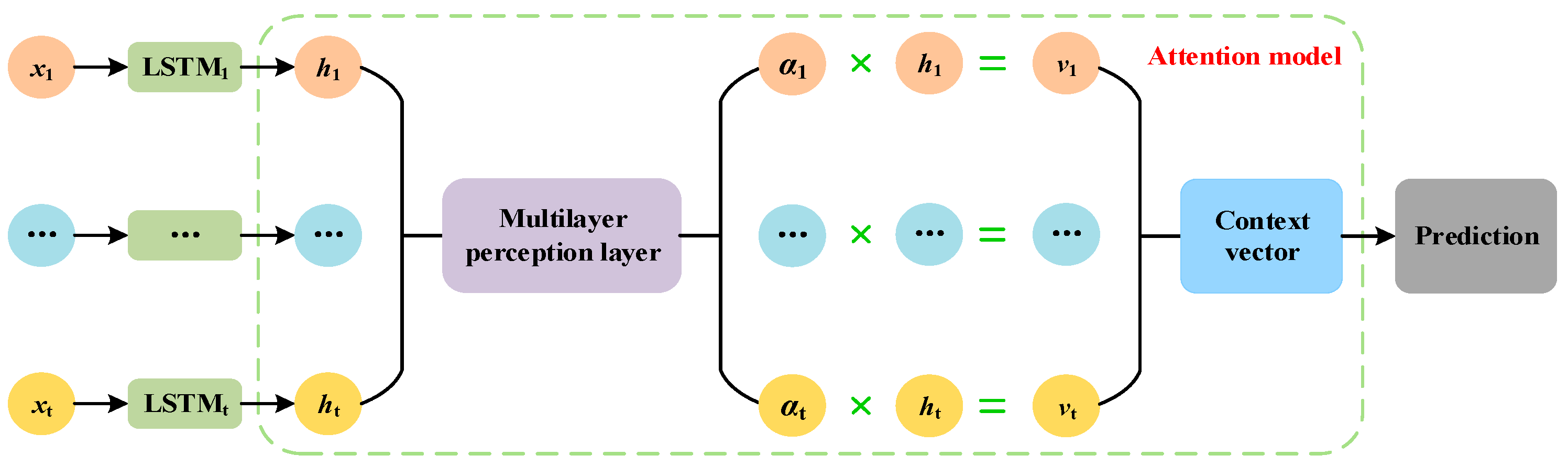
In summary, the nonlinear and nonstationary interference of the original subway passenger flow time series makes it difficult to improve the accuracy of the STPFP. A prediction method called IVMD-SE-MSSA based on IVMD time series decomposition and multi-model combination is proposed. Firstly, the elite opposition strategy, the new location update method, and the adaptive T distribution are introduced into SSA. The MSSA is used to optimize VMD parameters. Then, the IVMD is applied to decompose the original nonlinear and non-stationary passenger flow time series, and several stationary sub-series containing local features are obtained. The sub-series is divided into high-frequency and low-frequency components by SE. The low-frequency components are predicted by a back propagation (BP) neural network, and the high-frequency components are predicted by an attention LSTM (ALSTM). Finally, to further improve the prediction accuracy, the MSSA algorithm is used to combine the prediction results of each sub-series to obtain the final passenger flow prediction results. The major contributions of this paper are as follows:
(1) A mixed-strategy improved SSA algorithm is proposed to optimize the parameters of VMD. IVMD is applied to decompose the original passenger flow data to reduce the time variability and complexity of the passenger flow time series and improve predictability.
(2) The decomposed sub-series is divided into high-frequency and low-frequency components by SE, and different prediction models are used for different frequency components to avoid the limitation of one model.
(3) To further improve the prediction accuracy, a combination method based on MSSA is proposed to reduce the error superposition of the sub-series.
(4) To verify the validity of the established model, the passenger flow of four stations on the Nanning Metro was used to predict and four groups of comparative experiments were carried out. The experimental results showed that the prediction results of the established model were accurate and universal.
The rest of this paper is organized as follows. The theoretical background of the method used in this paper is introduced in Section 2. The proposed IVMD-SE-MSSA model is described in Section 3. The experiments and analysis are written in Section 4. Some conclusions and future work are given in Section 5.

2. Methodology

2.1. Problem Statement

STPFP is based on the historical passenger flow data of τ time intervals at subway stations, aiming at predicting the passenger flow of the next h time steps. In the time dimension, a one-dimensional time series is used to describe the inbound or outbound passenger flow of the stations, which can be expressed as:
X s = x t τ s , x t τ + 1 s , x t i s , , x t 1 s , x t s
where x t s represents the passenger flow of station s at the time t. The goal is to use sequence X s to establish a mapping function f to calculate the passenger flow in the next h time steps. It can be expressed by the following mathematical formula:
[ x t + 1 s , , x t + h s ] = f ( X s )

2.2. Variational Mode Decomposition

VMD is an adaptive signal processing method. It is essentially a process of constructing and solving variational problems. VMD can decompose the signal into k intrinsic mode functions (IMFs) with limited bandwidth to reduce the nonlinearity and nonstationarity of the original signal. It is widely used in the field of fault diagnosis and prediction. The decomposition effect of VMD is affected by the number of modal components k and the penalty factor α, so these two parameters need to be optimized. Dragomiretskiy et al. [34] and Jin et al. [54] introduced the related theories in detail.

2.3. MSSA Optimized VMD

2.3.1. SSA

The SSA algorithm is an optimization algorithm inspired by the foraging behavior and anti-predation behavior of sparrows. Assuming that there are n sparrows in the d-dimensional space, then the position of the i-th sparrow in the d-dimensional search space is xi = [x1, …, xid], where i = 1, 2, …, n. In each iteration, the position of the discover is updated as follows [47]:
x i , j t + 1 = x i , j t exp i α i t e r max , R 2 < S T x i , j t + Q L , R 2 S T
where t represents the current number of iterations, α is a random number evenly distributed between 0 and 1. R 2 [ 0 , 1 ] and S T [ 0.5 , 1 ] represent the warning and security values, respectively. Q is a random number with a normal distribution. L is a 1 × d matrix with 1 element, and itermax is the maximum number of iterations. When R2 < ST, it means that it is safe, and the discoverer can search widely. If R2ST, it means that there are predators at this time, and the sparrow population needs to quickly fly to other safe areas for foraging. The position of the participants is updated as follows:
x i , j t + 1 = Q exp x w o r s t x i j t i 2 , i > n / 2 x p t + 1 + x i , j x p t + 1 A + L , o t h e r w i s e
where xp and xworst represent the best position and the worst position occupied by the discoverer, respectively. A is a 1 × d matrix randomly assigned to 1 or −1 and A+ = AT(AAT)−1. When i > n/2, the i-th participant with a poor position cannot get food and needs to fly to other areas to find food. Assuming that the proportion of sparrows in the sparrow population that are aware of a hazard is 0.1–0.2, the positions of these sparrows are updated as follows:
x i , j t = x b e s t t + β x i , j t x b e s t t , f i > f 𝘨 x i , j t + K x i , j t x w o r s t t f i f w + ε , f i = f 𝘨
where x b e s t t represents the global best position of the current sparrow population, and β is a random number of a normal distribution with a mean of 0 and a variance of 1. fi represents the current sparrow fitness, K [ 1 , 1 ] , and fg and fw represent the global best and worst fitness, respectively. ε is a constant to avoid the denominator being 0.

2.3.2. MSSA

Due to the sparrow population initialization being randomly generated, this method will make the population distribution uneven, which directly affects the iterative optimization of the algorithm in the later stage. Therefore, the elite opposition strategy is used to initialize the sparrow population. Assuming that the elite individual in the population is x i , j e = ( x i , 1 e , x i , 2 e , , x i , d e ) (j = 1, 2, 3, …, d), its reverse individual x i , j e ¯ = x i , 1 e ¯ , x i , 2 e ¯ , , x i , d e ¯ can be defined as:
x i , j e ¯ = K α j + β j x i , j e
where K is the varying dynamic coefficient between 0 and 1, x i , j e [ α j , β j ] , and αj = min(xi,j) and βj = max(xi,j) are the dynamic boundaries. The dynamic boundaries overcome the shortcoming that the fixed boundaries are difficult to save the search experience, so that the elite opposition solution can be located in the narrow search space, which is conducive to the convergence of the algorithm. If the dynamic boundary operation makes x i , j e ¯ cross the boundary into an infeasible solution, it can be reset by a randomly generated method. The reset method is as follows:
x i , j e ¯ = r a n d ( α j , β j )
According to the discover position update formula of the SSA algorithm, when R2 < ST, each dimension of the discoverer becomes smaller and converges to 0. When R2ST, the discoverer will move randomly to the current position according to the normal distribution. This makes the algorithm tend to approach the global optimal solution at the beginning of the iteration, which can easily lead to premature convergence of the algorithm and a fall into a local optimum. Therefore, the position update strategy of the BOA global search phase is introduced to improve the position update formula of the discoverer in SSA. The improved position update method can be expressed as:
x i , j t + 1 = x i , j t + ( r 2 x b e s t t x i , j t ) f i , R 2 < S T x i , j t + Q L , R 2 S T
where r is a random number between 0 and 1, x b e s t t is the global optimal solution of the current iteration, and fi is the current fitness. The improved position update formula improves the defect of the lack of information exchange between individuals in the original algorithm and expands the search space. Besides, to improve the local search ability of the algorithm, an adaptive T distribution mutation strategy is introduced to update the position of sparrows, so as to improve the ability and robustness of the algorithm to jump out of the local optimum. The specific variation is as follows:
x i t = x i + x i t ( i t e r )
where x i t is the mutated sparrow position, xi is the sparrow i position, iter is the current iteration number, and t(iter) is the T distribution with the degree of freedom parameter as the iteration number.

2.3.3. MSSA-VMD

Envelope entropy [55] is an index used to evaluate the complexity of time series. When VMD decomposes the passenger flow time series, k IMF components are obtained. If the IMF component contains more noise, the envelope entropy is larger. Conversely, it is smaller. Therefore, the minimum envelope entropy is used as the fitness function for VMD parameter optimization. The envelope entropy Ep of the time series can be expressed as:
p j = a ( j ) / j = 1 N a ( j ) E p = j = 1 N p j lg p j
where aj is the decomposed subsequence signal, pj is the normalized form of aj, and N is the number of sampling points. After VMD decomposition, the minimum envelope entropy of the IMF component can be expressed as:
min I M F E p 1 , E p 2 , , E p k
Combined with the MSSA algorithm, the minimum envelope entropy of the IMF component is taken as the objective function to optimize the modal component k and penalty factor α of VMD. The optimization process can be regarded as a nonlinear unconstrained optimization. The specific steps are as follows:
Step 1: The elite opposition learning strategy is used to initialize the population while initializing the number of iterations, predators, and adders. Set the range of k and α that needs to be optimized.
Step 2: Calculate and sort the fitness values of each sparrow to determine the current best fitness value and its corresponding position.
Step 3: Select the part of the sparrow with better fitness as the discoverer, and use Equation (8) to update the position of the discoverer.
Step 4: The remaining sparrows are participants, and the position is updated according to Equation (4).
Step 5: Some sparrows are randomly selected from the whole population as alerters, and the position is updated according to Equation (5).
Step 6: After iteration, the global optimal sparrow is calculated and found, and the adaptive T distribution mutation is carried out.
Step 7: The best position and the best fitness of the sparrow population are updated. If the maximum number of iterations is reached, the optimal result is output, otherwise return to step 2 to iterate again.

2.4. Prediction Models

2.4.1. BP Neural Network

BP neural network is a shallow machine learning model, it is a three-layer neural network. In general, BP neural network can approximate any nonlinear function [56]. Its network structure consists of input layer, hidden layer, and output layer. In the modeling process, BP neural network is used to construct nonlinear function. The calculation formula is as follows:
Y = c 1 + w 1 ( f 1 ( c 2 + w 2 × X ) )
where w1 and w2 are the weights of the output layer and the hidden layer, respectively. c2 and c1 are the biases of the hidden layer and the output layer, respectively. f1 is the activation function.

2.4.2. Attention Long Short-Term Memory Neural Network

LSTM is a variant of RNN that effectively solves the problems of gradient disappearance and gradient explosion [57]. The core of LSTM is that it adds a memory unit and protects and controls the state of the memory unit through a forget gate (ft), input gate (it), and an output gate (Ot). Its basic structure is shown in Figure 1. The basic principle of LSTM can be written as:
f t = σ ( W f h t 1 , x t + b f ) i t = σ ( W i h t 1 , x t + b i ) C ˜ t = tanh ( W C h t 1 , x t + b C ) C t = f t C t 1 + i t C ˜ t O t = σ ( W O h t 1 , x t + b O ) h t = O t tanh ( C t ) y ^ t = W y h t + b y
where C ˜ t is a new candidate value vector fortheunit state. Ct represent the cell status, xt and ht represent input and output, respectively, y ^ t is the predicted value, W is the weight matrices, b is the bias vectors. * represents the scalar product, and σ is the sigmoid function.
In order to enable LSTM to extract different weights of features, an attention mechanism [58] is added after the LSTM layer to capture long-term time dependencies. As shown in Figure 2, assuming that the output of the LSTM hidden state is h1, …, ht. The output is used as the input of the attention mechanism. The multilayer perceptron (MLP) is used to learn the weight of each hidden state, and the output is obtained through the MLP layer. The output can be expressed as:
u i = v u tanh ( w u h i + b u ) , i [ 1 , t ]
where wu, bu, and vu are learnable parameters, and tanh is the activation function.
The weight of each output series is calculated by the Softmax normalized exponential function, which can be expressed as:
α i = Softmax ( u i ) = exp ( u i ) k = 1 t exp ( u k )
Then, the context vector V with global dynamic temporal dependencies can be calculated by weighted sum, which can be expressed as:
V = i = 1 t α i h i
Finally, the context vector V is input to the full connection layer to obtain the output prediction value. The addition of the attention mechanism enables the LSTM to filter useful information in all hidden states, and the weight of the filtering will change according to changes in the input information. This enables the LSTM to capture the long-term dynamic time dependencies, which solves the defects of the LSTM.

2.5. Sample Entropy

SE is often used to measure the complexity of time series [53], and its pseudo-mathematical expression is as follows:
S E = E ( v , m , r )
where v is a time series and m is the embedding dimension. The similarity tolerance r is set to 0.2std, where std is the standard deviation of the time series.

3. The Process of the Proposed Model

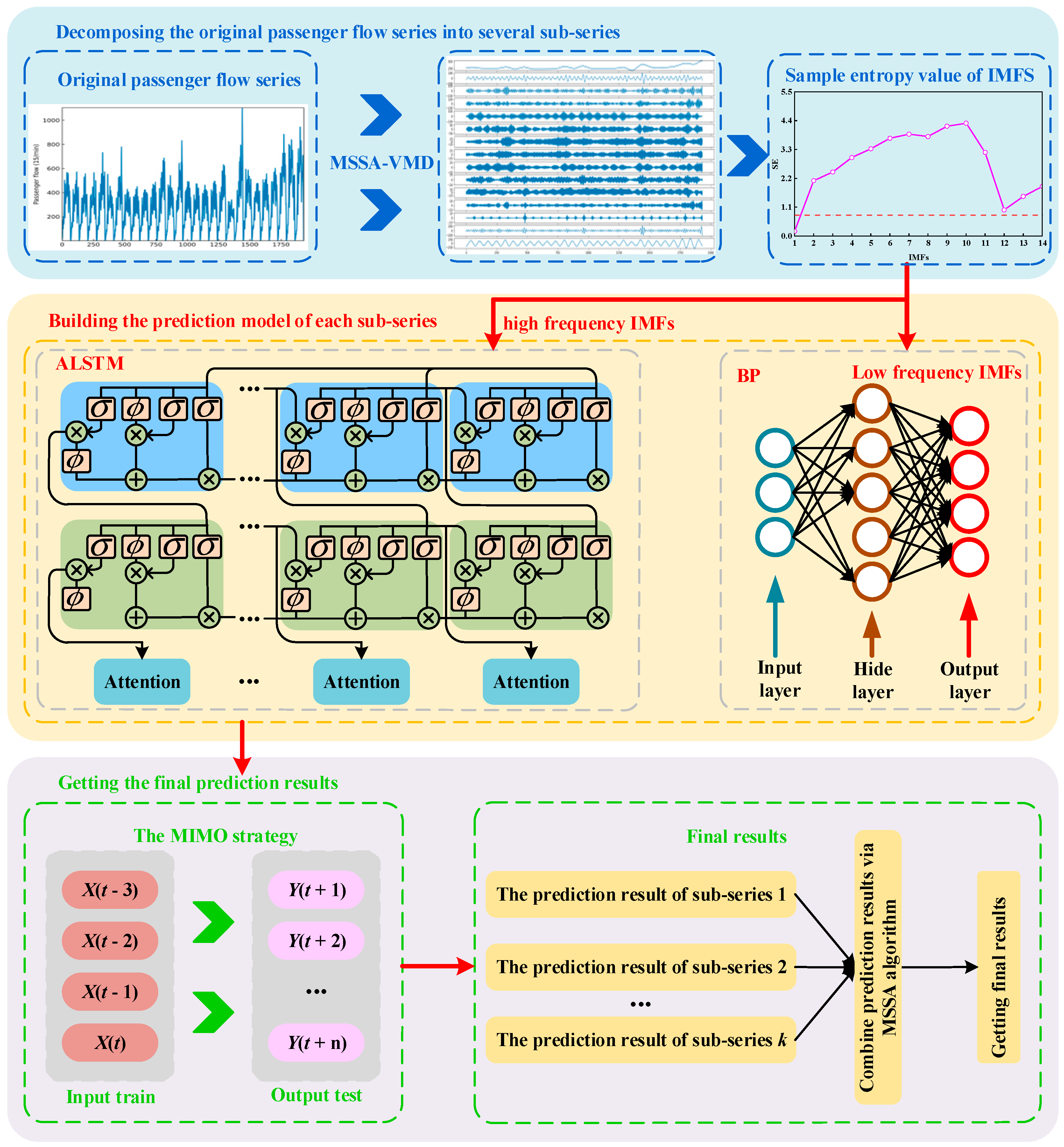
The proposed IVMD-SE-MSSA model architecture is shown in Figure 3. The modeling steps of the whole process are as follows:
Step 1: Taking the minimum envelope entropy as the optimization objective, the MSSA algorithm is used to search for the parameters of VMD.
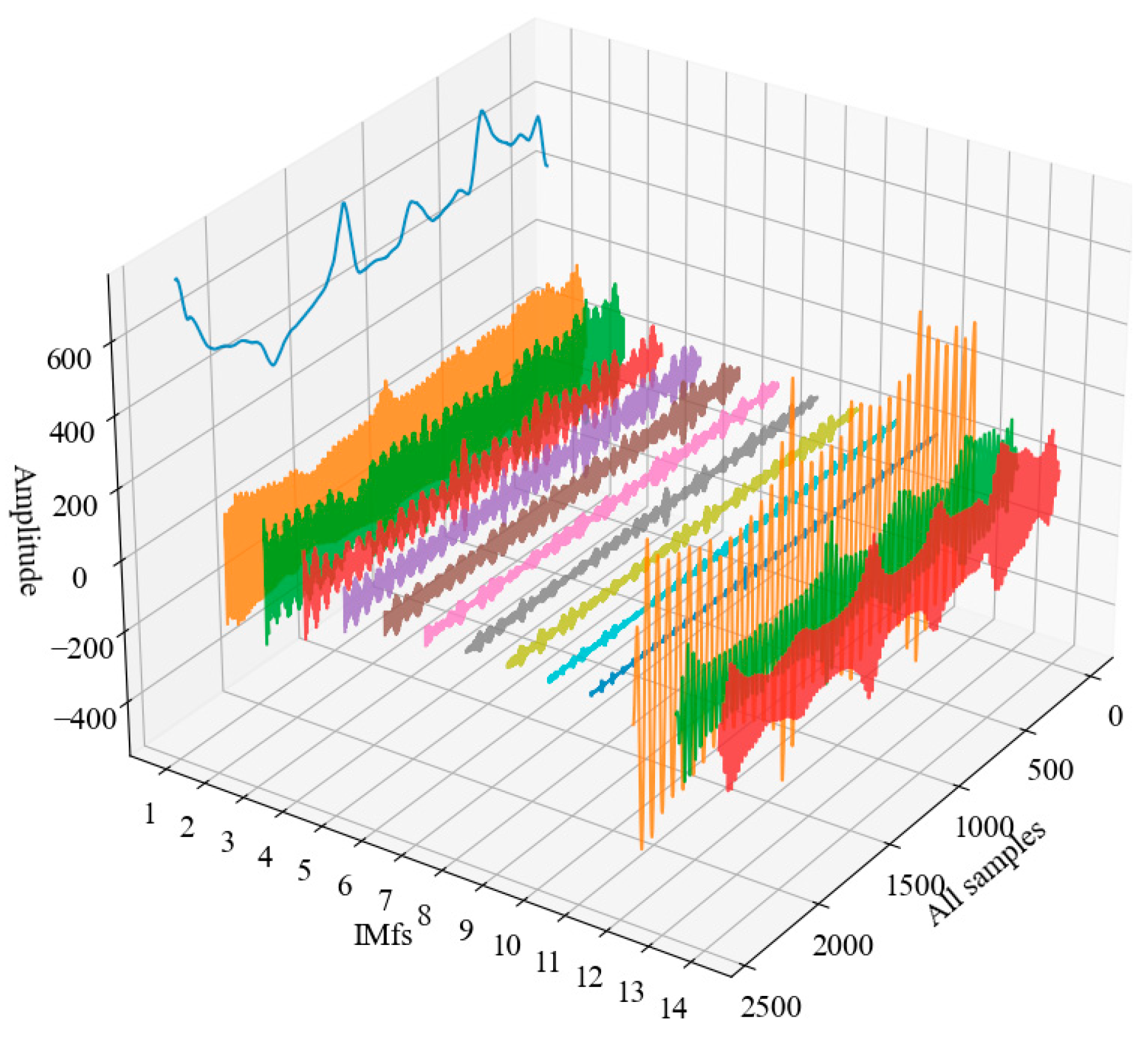
Step 2: After searching for the optimal parameters, the IVMD is used to decompose the passenger flow time series, and k IMF components are obtained.
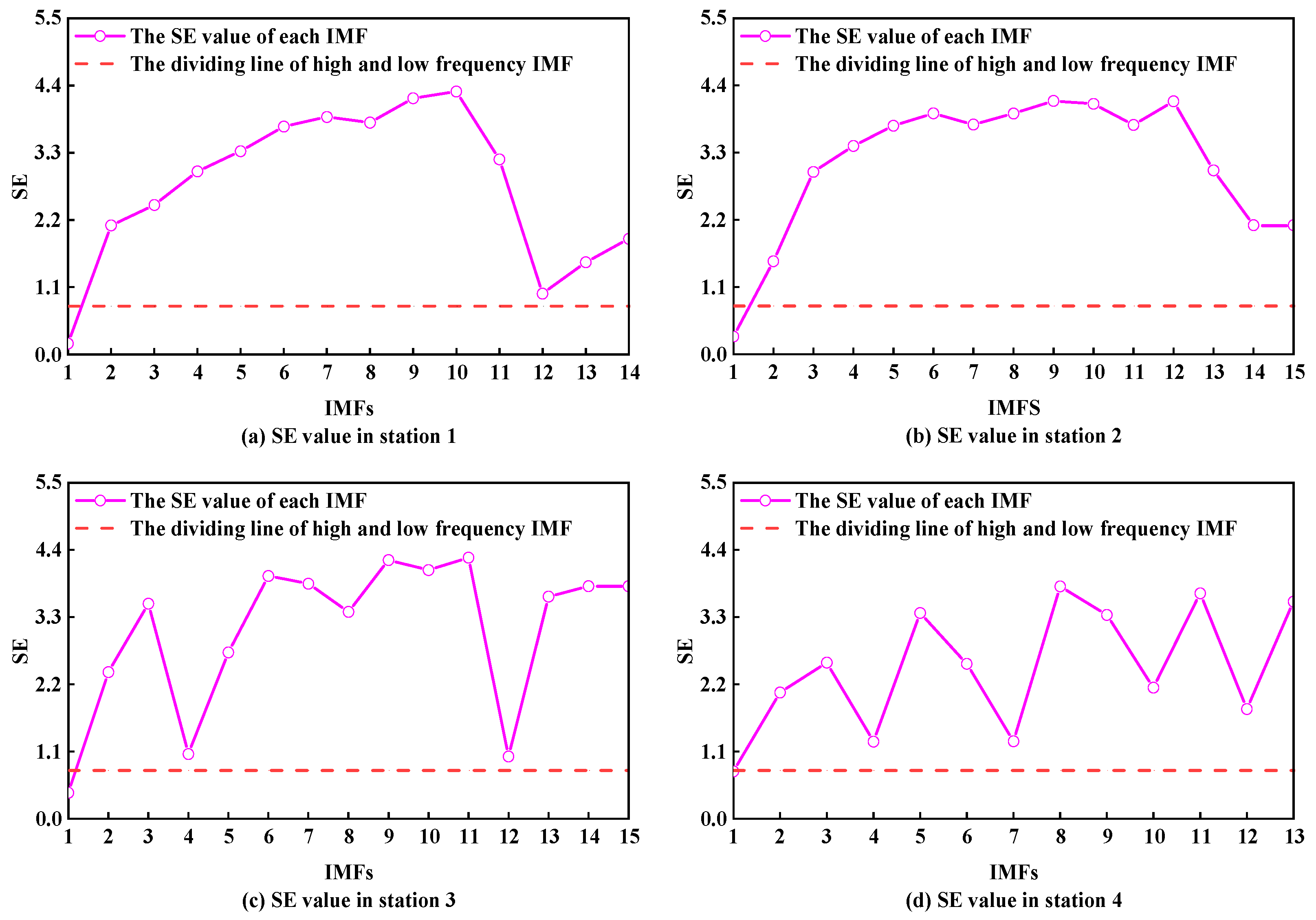
Step 3: Calculate the SE value of each IMF component. The IMF is divided into high-frequency and low-frequency IMFs by SE value.
Step 4: BP is used to predict the low-frequency components, and ALSTM is used to predict the high-frequency components. Besides, in the prediction process, a multi-input multi-output (MIMO) strategy [59] is used for multi-step prediction. In the field of time series prediction, the cumulative error of the MIMO strategy is very small [60].
Step 5: MSSA is used to combine the prediction results of each component to obtain the final prediction results. In the study of pattern decomposition and multi-model combination forecasting methods, the weight of each prediction model is set to 1. This means that all prediction models have the same importance or prediction performance. However, the prediction accuracy of each prediction model is different, and the importance of different models in accumulating final prediction values is also different. Therefore, if each prediction model assigns appropriate weight coefficients according to certain rules, the final prediction accuracy can be improved. Based on the work of Zsuzsa et al. [61], Precup et al. [62], and Sawulski et al. [63], the root mean square error between the actual value and the predicted value is taken as the optimization object, and the MSSA algorithm is introduced to optimize the weight coefficient of each prediction model. The optimization problem can be regarded as a nonlinear constrained optimization problem.
Assuming that yt (t = 1, 2, …, N) is the actual passenger flow time-series data, and N is the number of sample points. y ^ i t is the predicted value of the ith sub-series, and e i t = y t y ^ i t is the prediction error. wi is the weight coefficient of the ith sub-series prediction model. Then, the optimization problem of the combination prediction model can be defined as:
Minimize 1 N t = 1 N ( i = 1 k w i ( y i t + e i t ) i = 1 k w i y ^ i t ) 2 subject to { 2 w i 2 } , i = 1 , 2 , , k
The optimization process stops when the maximum number of iterations is reached, and it can be terminated according to predefined conditions. At this time, the weight coefficient of each subsequence is obtained, and the prediction result of the final model can be expressed as:
y ^ t = i = 1 k w i y ^ i t , t = 1 , 2 , , N
where y ^ t is the prediction result of the combined model, and wi is the weight coefficient of the ith sub-sequence prediction model optimized by the final MSSA.

4. Experiments

In the section, some important information is first introduced, including dataset descriptions, evaluation indicators, and some experimental parameter configurations. Then, the performance of the IVMD-SE-MSSA model is evaluated by experiments. All the experiments in this paper were carried out on a Linux server (CPU: i9-10900X, GPU: RTX 3090). The proposed model was developed by Keras, and the code of the algorithm can be downloaded at https://github.com/wjx-mel/IVMD-SE-MSSA, accessed on 20 March 2023.

4.1. Datasets

The experimental datasets are from Chaoyang Square Station (Station 1), Nanning East Station (Station 2), Nanning Railway Station (Station 3), and Jinhu Square Station (Station 4) of the Nanning Metro Line 1. The selection of these stations is helpful to verify the universality of the proposed model. The AFC data from 2 August to 29 August 2021, are used for experiments in the study. Since the operation time of Nanning Metro Line 1 is 6:30–23:00, the inbound passenger flow data from 6:30 to 23:30 are filtered and retained. Besides, the data are aggregated to 15 min. There are 1932 continuous data points in each dataset time series, of which 1449 data points in the first three weeks are used for training and 483 data points in the fourth week are used for testing. The detailed characteristics of the data are shown in Table 1. The original passenger flow datasets are shown in Figure 4. It can be seen from Figure 4 that Chaoyang Square Station (Station 1) is a transportation hub, and its inbound passenger flow presents bimodal characteristics. This station is located in the urban area of Nanning City and is the subway station with the highest daily passenger flow. Nanning East Station (Station 2) and Nanning Railway Station (Station 3) are close to large high-speed railway stations, and their passenger flows have no obvious regularity and significant differences. Jinhu Square Station (Station 4) is close to the commercial area, and many people commute nearby. Therefore, the passenger flow at the station shows an evening peak on the working day. The obvious evening peak characteristics make the regularity of the passenger flow at the station very significant, which helps to improve the prediction performance. In addition, it can be clearly seen from Figure 4 that the passenger flow data sets of the four stations are strongly nonlinear and non-stationary.

4.2. Evaluating Metric

The mean absolute error (MAE), mean absolute percentage error (MAPE), root mean square error (RMSE), and standard deviation of error (SDE) were used to evaluate the prediction performance of the proposed model. The definitions are listed in Equations (20)–(23):
M A E = 1 N t = 1 N y ^ t y t
M A P E = 1 N t = 1 N y ^ t y t y t
R M S E = 1 N t = 1 N ( y ^ t y t ) 2
S D E = 1 N t = 1 N y t y ^ t 1 N t = 1 N ( y t y ^ t ) 2
where y ^ t and yt represent thepredicted value and actual value, respectively. N denotes the totalamount of the data to be predicted.

4.3. Model Configuration

In the experiment, the model parameters involved in the experiment were selected by reference and control variable method. In the hybrid model IVMD-SE-MSSA, MSSA was used to optimize the k and α of the VMD, searching for k between 1 and 20, and searching for α between 1 and 5000. In MSSA, the proportion of discoverers was set to 0.8, the warning value was set to 0.6, the proportion of alerters was set to 0.8, the search dimension was two-dimensional, the population size was set to 30, and the maximum number of iterations was set to 20. The ALSTM had two hidden layers, and the number of neurons in the hidden layer was 64. The batch size was set to 16, the time step was set to 5, and the prediction step was set to 3. That is, the first five time steps were used to predict the next three time steps. The optimizer used Adam and used mean-square error (MSE) as the loss function. The epochs were set to 250, and the learning rate was set to 0.001. Besides, a dropout layer was added to prevent model overfitting. When combining the prediction results of sub-series, the search dimension of MSSA was set to k, the population size was set to 300, and the maximum number of iterations was set to 1000. The weight coefficients were searched between −2 and 2.

4.4. Results and Discussion

4.4.1. Optimization Result of VMD by MSSA

To prove the effectiveness of the MSSA algorithm, four test functions are selected for simulation analysis. The test functions are shown in Table 2. In addition, in order to prove the optimization ability of the MSSA algorithm, SSA, GWO, PSO, and bat algorithm (BA) [64] were selected for comparative analysis. The population size is set as 30, the maximum number of iterations is 500, and the dimension is 30. The specific parameters of each algorithm are shown in Table 3. F1(x) is a unimodal function. Its global optimal solution is surrounded by local extrema, which makes it difficult to find the optimal solution. F2(x), F3(x), and F4(x) are multimodal functions, where F2(x) and F3(x) have many local extreme values, and the number of local extreme values of F4(x) increases with the increase of dimension. Therefore, these four test functions have a certain difficulty in solving, which makes them suitable for testing the optimization performance of the algorithm. The convergence curves of each algorithm for four functions are shown in Figure 5. It can be seen from Figure 5 that the MSSA always shows a better convergence speed than other optimization algorithms for each test function. This is because the elite opposition strategy makes the group size adaptive to change, and ordinary individuals will accelerate the movement toward elite individuals. Moreover, MSSA can always achieve the theoretical optimal value, which is mainly due to the adaptive T distribution mutation strategy, giving it the ability to jump out of the local optimum. In summary, the proposed MSSA optimization algorithm has a faster convergence speed and stronger global search ability, which gives it greater advantages in optimization performance.
To obtain the best parameter combination of VMD k and α, MSSA is used to get the best parameters of VMD. The optimized convergence curves for the four station datasets are shown in Figure 6. It can be seen from Figure 6 that the MSSA algorithm has reached the optimal value, which proves that the MSSA optimization algorithm has strong optimization ability. Taking station 1 as an example, it can be seen from Figure 6 that MSSA converges after the 6th iteration, and the corresponding fitness value is 2.9501. SSA, GWO, PSO, and BA converge after the 8th, 12th, 12th, and 10th iterations, and the corresponding fitness values are 2.9512, 2.9522, 2.9542, and 2.9571, respectively. At station 2, it can be seen from Figure 6 that MSSA converges after the 3rd iteration, and the corresponding fitness value is 2.9716. SSA, GWO, PSO, and BA converge after the 9th, 12th, 5th, and 12th iterations, and the corresponding fitness values are 2.9728, 2.9739, 2.9745, and 2.9751, respectively. At station 3, it can be seen from Figure 6 that MSSA converges after the 7th iteration, and the corresponding fitness value is 3.0894. SSA, GWO, PSO, and BA converge after the 8th, 10th, 11th, and 10th iterations, and the corresponding fitness values are 3.0963, 3.0978, 3.1028, and 3.104, respectively. At station 4, it can be seen from Figure 6 that MSSA converges after the 9th iteration, and the corresponding fitness value is 2.8945. SSA, GWO, PSO, and BA converge after the 14th, 11th, 6th, and 9th iterations, and the corresponding fitness values are 2.8955, 2.8976, 2.8987, and 2.9, respectively. Compared with other algorithms, MSSA has faster convergence speed and global optimization ability, which proves that the proposed mixed strategy improved SSA is very effective. According to the optimization results, the corresponding k and α values on the four datasets are selected as shown in Table 4.

4.4.2. IVMD Decomposition Results and SE Calculation Results

According to the optimal parameter combination of VMD, the original passenger flow time series is decomposed by IVMD. The decomposition results of the four stations are shown in Figure 7, Figure 8, Figure 9 and Figure 10. Each figure is IMF1 to IMFk from top to bottom. It can be seen from the figures that the sub-series decomposed by IVMD are more stable and regular, which helps to improve the predictability of time series.
IVMD decomposes a finite number of IMF components with different complexity. Using appropriate models for sub-series with different complexity helps to exert the ability of the model itself and improve the prediction performance of the model. The SE calculation results of each IMF component in the four datasets are shown in Figure 11. It can be seen from Figure 11 that SE increases with the increase of model components, which indicates that the complexity of sub-series is gradually increasing. In the study, different values were selected in [0.1, 0.2, 0.3, …, 0.9, 1] to determine the SE threshold. Through many experiments, the SE threshold was set to 0.8, lower than 0.8 for low-frequency components and higher than 0.8 for high-frequency components. In Figure 11, above the red dotted line are the high-frequency components, and below the dotted line are the low-frequency components. It can be seen from Figure 11 that the first component of the four datasets is the low-frequency component, and the rest are the high-frequency components. Therefore, BP is used to predict the low-frequency components, and ALSTM is used to predict the high-frequency components.

4.4.3. Experiment 1: Comparison of Prediction Performance with Different Single Models

The purpose of experiment 1 is to compare the predictive ability of the proposed IVMD-SE-MSSA model with several classic single prediction models, including the BP, LSTM, and ALSTM models. BP has only one hidden layer with a size of 64. The parameter settings of the LSTM are the same as those of the ALSTM. These models consider shallow machine learning methods and deep learning methods to comprehensively compare the proposed model with several classical prediction models. The experimental results are shown in Table 5, where the bold part is the best prediction result.
For station 1, IVMD-SE-MSSA achieves the most satisfactory prediction accuracy in one-step prediction. In the two-step and three-step predictions, the evaluation index of IVMD-SE-MSSA is also the lowest relative to other comparison models. This means that the IVMD-SE-MSSA model is very effective for passenger flow prediction. In the subway station passenger flow prediction, it is necessary to preprocess the original passenger flow time series. After data preprocessing, the prediction accuracy can be significantly improved. For single models, BP is a shallow machine learning model, which is more suitable for predicting stationary time series. For time series with high complexity, its prediction performance is poor, and its one-step prediction MAPE is 0.8734. The MAPE predicted by LSTM in one-step is 0.7358. ALSTM adds attention to better process the input sequences. In one-step prediction, the MAPE of ALSTM is 0.6545. The MAPE of IVMD-SE-MSSA is 0.0328, which is 96.24%, 95.54%, and 94.99% better than that of BP, LSTM, and ALSTM, respectively. Figure 12 shows the predicted values, scatter plots, and evaluation index comparison of the model involved in station 1. It can be seen from Figure 12 that the performance of IVMD-SE-MSSA is significantly better than that of single models.
For station 2, the MAPE values of BP, LSTM, and ALSTM are 5.9772, 3.2528, and 2.6472, respectively, in the two-step prediction. In contrast, the MAPE value of IVMD-SE-MSSA is 0.0698, which has a greater predictive advantage than the above model. In addition, the prediction error of single models increases exponentially with the prediction step size, while IVMD-SE-MSSA does not change as dramatically.
For station 3, based on the four evaluation indices, the proposed model is still superior to other related models. In the three-step prediction, the MAE, MAPE, RMSE, and SDE values of IVMD-SE-MSSA are 6.4835, 0.0417, 7.944, and 7.9443, respectively. In the remaining single models, the prediction accuracy from good to bad is ranked as ALSTM, LSTM, and BP, and the MAPE values are 0.758, 0.5808, and 0.5272, respectively.
For station 4, from one-step prediction to three-step prediction, the MAPE values of IVMD-SE-MSSA are 0.0325, 0.043, and 0.0646, respectively. Compared with the ALSTM with the best MAPE value in the single models, the prediction accuracy of the IVMD-SE-MSSA model improved by 66.9%, 80.32%, and 80.43% from one-step to three-step prediction, respectively.
The prediction results of experiment 1 show that the prediction performance of IVMD-SE-MSSA is significantly different from that of other single models. Specifically, no matter what kind of prediction step, IVMD-SE-MSSA obtain significantly higher satisfactory evaluation index values. Therefore, it can be concluded from experiment 1 that the combined model based on advanced data preprocessing technology has better ability than single models in short-term passenger flow prediction. Data preprocessing techniques can help reduce the nonlinearity and nonstationarity of time series and significantly improve the prediction performance.

4.4.4. Experiment 2: Comparison with Other Combined IVMD Prediction Models

The purpose of experiment 2 is to study the performance of other prediction models after IVMD decomposition. The IVMD-BP, IVMD-ALSTM, and IVMD-SE models are constructed in the experiment. Instead of using SE to divide high-frequency and low-frequency components, IVMD-BP and IVMD-LSTM predict all sub-series directly using BP and ALSTM. IVMD-SE directly superimposes the prediction results of sub-series without using MSSA to combine the prediction results of each sub-series. In addition, the parameters of IVMD, BP, ALSTM, and LSTM are the same as the above settings. The experimental results are shown in Table 6.
For station 1, the predictive performance of IVMD-BP is better than that of IVMD-ALSTM. This is because neither IVMD-BP nor IVMD-ALSTM uses SE to distinguish between high- and low-frequency components but instead uses a model directly for prediction. According to the above IVMD decomposition and SE calculation results, it can be found that IMF1 is always a low-frequency component, and the rest is a high-frequency component. The low-frequency component contains more inherent characteristics of a time series signal, which play an important role in prediction. Therefore, accurate prediction of low-frequency components is particularly important for the prediction performance of the final model. The prediction of low-frequency components by ALSTM is prone to over-fitting, which has a great impact on the final prediction results. BP is more suitable for stationary time series. Thus, the predictive performance of IVMD-BP is better than that of IVMD-ALSTM. This also reflects the importance of using SE to make different models predict different complexity sub-series. In addition, the prediction performance of IVMD-SE is not as good as that of IVMD-SE-MSSA, which indicates that the MSSA algorithm can effectively combine the prediction results of different models and further improve the prediction performance of the model. In the three steps of prediction, the MAPE of IVMD-SE-MSSA is 0.0328, 0.0397, and 0.0519, respectively, which is better than 0.0487, 0.0459, and 0.0779 for IVMD-SE.
For Station 2, IVMD-SE-MSSA obtains the best four evaluation criteria under the three steps prediction. Specifically, in one-step prediction, the MAPE of the IVMD-SE-MSSA is 0.0734, while the MAPE of the IVMD-BP, IVMD-ALSTM, and IVMD-SE is 0.4598, 0.5009, and 0.3253, respectively. Compared with them, the prediction accuracy of the IVMD-SE-MSSA is improved by 84.04%, 85.35%, and 77.44%. Figure 13 shows the prediction results of different prediction models using IVMD decomposition technology in station 2 and compares the corresponding evaluation indicators.
For station 3, it can be seen from Table 5 that IVMD-SE-MSSA has obtained the lowest evaluation metric in the three prediction steps. No matter which prediction steps are taken, IVMD-SE-MSSA can always provide the best prediction results.
For Station 4, the IVMD-SE-MSSA model has the best prediction performance compared with other hybrid models. For example, in the three-step prediction, the MAE, MAPE, RMSE, and SDE of the IVMD-SE-MSSA are 5.1648, 0.0646, 6.8261, and 6.7915, respectively, while the optimal IVMD-SE in the comparison model obtains only 7.0347, 0.0748, 9.6286, and 8.9105.
The prediction results and evaluation indices of experiment 2 show that the complexity analysis of sub-series and the combination of MSSA sub-series prediction results can further improve the prediction accuracy.

4.4.5. Experiment 3: Comparison of Hybrid Models with Different Data Preprocessing Techniques

Experiment 3 aims to compare the prediction performance of the hybrid model based on IVMD decomposition with the prediction performance of the hybrid model based on other data decomposition techniques, including the hybrid strategy of EMD, EEMD, CEEMADAN, and WD. The EMD, EEMD, and CEEMADAN are all based on Python’s PyEMD toolkit to automatically obtain their decomposition results. WD decomposes data according to Python’s pywt toolkit, referring to the research of Yang et al. [26], and Dmeyer is selected as the wavelet function in the experiment, and the decomposition depth is 5. Besides, each decomposition strategy uses the same SE and MSSA combination strategy. The experimental results are shown in Table 7.
Table 7 shows the prediction evaluation index values of the hybrid model composed of various data preprocessing techniques. For Station 1, the hybrid model based on IVMD is more accurate and effective in passenger flow prediction, and its MAPE values in the three steps prediction are 0.0328, 0.0397, and 0.0519, respectively. In contrast, the prediction performance of the hybrid model using WD technology is closely followed by that of IVMD-SE-MSSA, and its MAPE is 0.0604, 0.3195, and 0.4149, respectively. The MAPE of the EMD hybrid model is 0.2499, 0.4267, and 0.4741, respectively. The MAPE of the EEMD hybrid model is 0.2345, 0.3368, and 0.4467, respectively. The MAPE of the CEEMDAN hybrid model is 0.2538, 0.444, and 0.7221, respectively. These have a big gap with the IVMD decomposition strategy. Besides, with the increase of prediction steps, the prediction performance of the hybrid model based on EMD, EEMD, and CEEMDAN is very poor. The more prediction steps, the greater the error of the combined model. This shows that the hybrid model based on EMD has very unstable prediction ability.
For Station 2, IVMD-SE-MSSA also achieves the best prediction performance in the three steps prediction. In the three-step prediction, the MAPE of IVMD-SE-MSSA is 0.2221, while the MAPE of the hybrid model based on EMD, EEMD, CEEMDAN, and WD is 1.66, 0.976, 1.478, and 0.8509, respectively. Compared with them, the prediction accuracy of IVMD-SE-MSSA is improved by 86.62%, 77.24%, 84.97%, and 73.9%, respectively.
For Station 3, IVMD-SE-MSSA also has the best prediction performance. In the three-step prediction, the MAE, MAPE, RMSE, and SDE of IVMD-SE-MSSA are 6.4835, 0.0417, 7.9444, and 7.9443, respectively, while the best WD-SE-MSSA in the comparison model achieves only 13.3639, 0.0928, 17.35, and 17.3492. Figure 14 shows the prediction results of different data preprocessing hybrid models in station 3 and compares the corresponding evaluation indices.
For Station 4, it can be observed from Table 6 that the IVMD hybrid strategy has significant advantages, and this advantage is continuously amplified as the prediction step size increases. In the three steps of prediction, the MAPE of IVMD-SE-MSSA is 0.0325, 0.043, and 0.0646, respectively, and the optimal WD-SE-MSSA in the comparison model is 0.0494, 0.0846, and 0.1104, respectively. The worst EMD-SE-MSSA values are 0.0904, 0.1895, and 0.2527, respectively. The decomposition strategy based on IVMD has stable advantages.
The prediction results and evaluation indicators of experiment 3 show that the decomposition strategy based on IVMD is always superior to the decomposition strategy based on other data preprocessing techniques. Moreover, the decomposition strategy based on IVMD has very stable prediction ability.

4.4.6. Experiment 4: Comparison with Models Using Different Optimization Algorithms

The purpose of experiment 4 is to compare the model based on MSSA combined sub-series prediction results with the model based on other optimization algorithms. Similarly, the SSA, GWO, PSO, and BA are used for comparison in this section. The parameters of these algorithms are consistent with those in Table 3 above. Table 8 shows the evaluation index values for each combination strategy. It can be seen from the table that the prediction performance of the combination model is closely related to the optimization performance of the optimization algorithm. The better the optimization performance of the optimization algorithm, the better the final prediction performance of the combined model. The proposed MSSA has the best optimization ability, so IVMD-SE-MSSA has the best prediction performance. Figure 15 compares the prediction performance of various optimization algorithm combination models at station 4.
In addition, for the four station datasets and all prediction steps, the model based on the MSSA optimization algorithm has the most satisfactory MAE, MAPE, RMSE, and SSE values. In other words, the proposed model has remarkable adaptability for short-term subway passenger flow prediction. It is worth noting that the MSSA algorithm has lower prediction error and higher prediction accuracy, which is significantly better than the simple SSA algorithm.

4.5. Improvements from Proposed IVMD-SE-MSSA Model

In this section, four indicators (PMAE, PMAPE, PRMSE, and PSDE) are used to discuss in detail the accuracy and effectiveness of the proposed IVMD-SE-MSSA model. PMAE, PMAPE, PRMSE, and PSDE represent the percentage improvement of MAE, MAPE, RMSE, and SSE, respectively. The mathematical formulas of the indicators involved are shown in Table 9. In Table 9, MAE1, MAPE1, RMSE1, and SDE1 are the values of the proposed model prediction accuracy evaluation index, and MAE2, MAPE2, RMSE2, and SDE2 are the values of the compared model. On this basis, the detailed percentage of error improvement compared to all comparison methods is calculated, as shown in Table 10. With the increase in the improved percentage value, the prediction accuracy of the IVMD-SE-MSSA model is also improved compared with the baseline method. According to the calculation results in Table 10, compared with other baseline models, the developed IVMD-SE-MSSA model greatly improves prediction accuracy. The percentage of improvement relative to all comparison models and all stations is very prominent.

4.6. Statistical Test

In order to further evaluate the significance of the proposed IVMD-SE-MSSA method compared with other methods, the Diebold-Mariano (DM) [65] test is used to test whether there are significant differences between IVMD-SE-MSSA and the comparison method used in this paper. The three-step predicted DM values for the four datasets are shown in Table 11. It can be seen from Table 11 that, except for IVMD-SE-SSA, IVMD-SE-MSSA is significantly different from all other comparison models at the 1% significance level. Compared with IVMD-SE-SSA, IVMD-SE-MSSA can still significantly improve the prediction performance at a 5% or 10% significance level. Therefore, based on the analysis of all cases, it can be concluded that there are significant differences between the established IVMD-SE-MSSA method and other related models. This verifies the advantages of the proposed short-term passenger flow prediction model.

5. Conclusions

Aiming at the nonlinear and nonstationary interference of subway passenger flow time series, it is difficult to improve the accuracy of short-term passenger flow prediction. A hybrid prediction method IVMD-SE-MSSA is proposed. Specifically, IVMD technology is used to decompose the original passenger flow series to improve the predictability of the sequence. Then, the complexity of sub-series is divided by SE, and sub-series with different complexity are predicted, respectively. Finally, the MSSA is applied to combine the prediction results of each sub-series to get the final prediction results. In addition, some comparative models are designed to verify the performance of the proposed model. The main conclusions are summarized as follows:
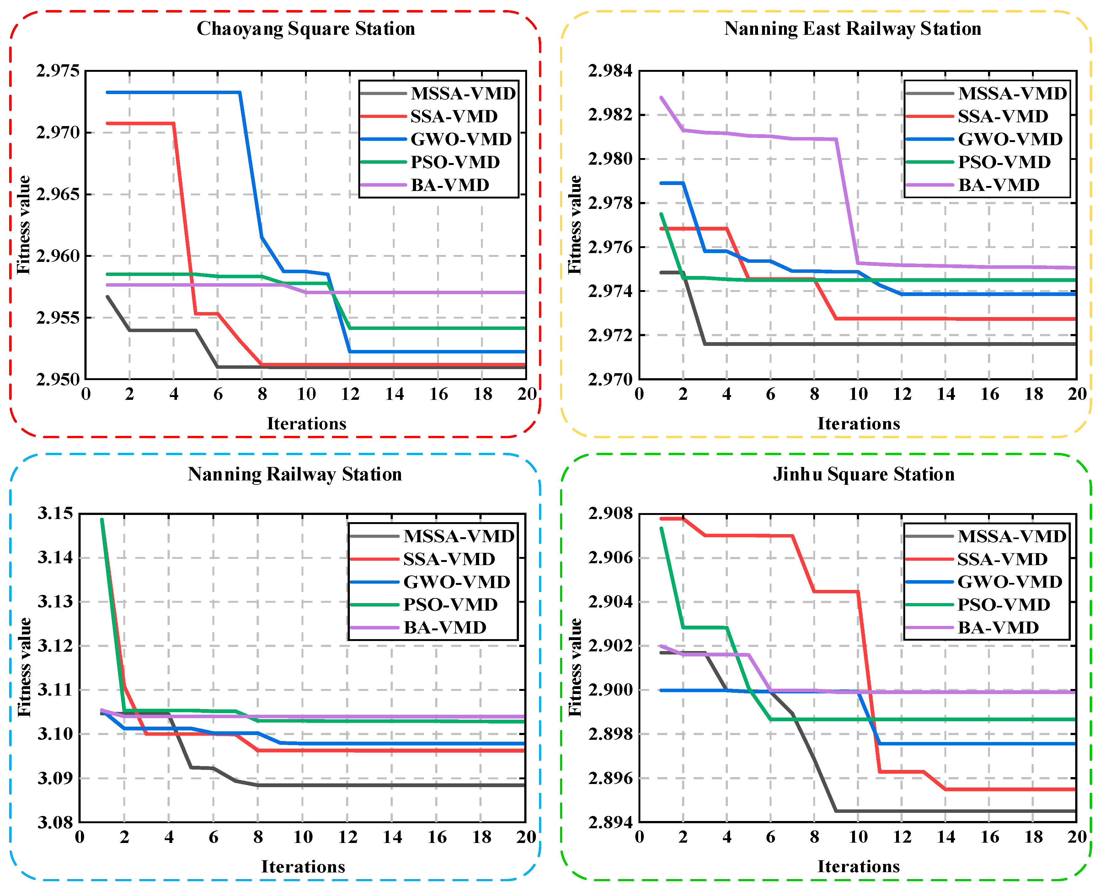
(1) The elite opposition strategy, the new position update method, and the adaptive T distribution mutation are introduced into SSA, and MSSA is proposed to optimize VMD. Compared with other optimization algorithms, MSSA has a faster convergence speed and higher optimization accuracy.
(2) The optimized adaptive VMD is used to decompose the original passenger flow time series. The experimental results showed that IVMD has a more stable prediction effect than other data preprocessing methods.
(3) The sub-series are divided by SE, and the prediction results of the sub-series are combined by MSSA. Experimental results show that both of them can further improve the prediction accuracy.
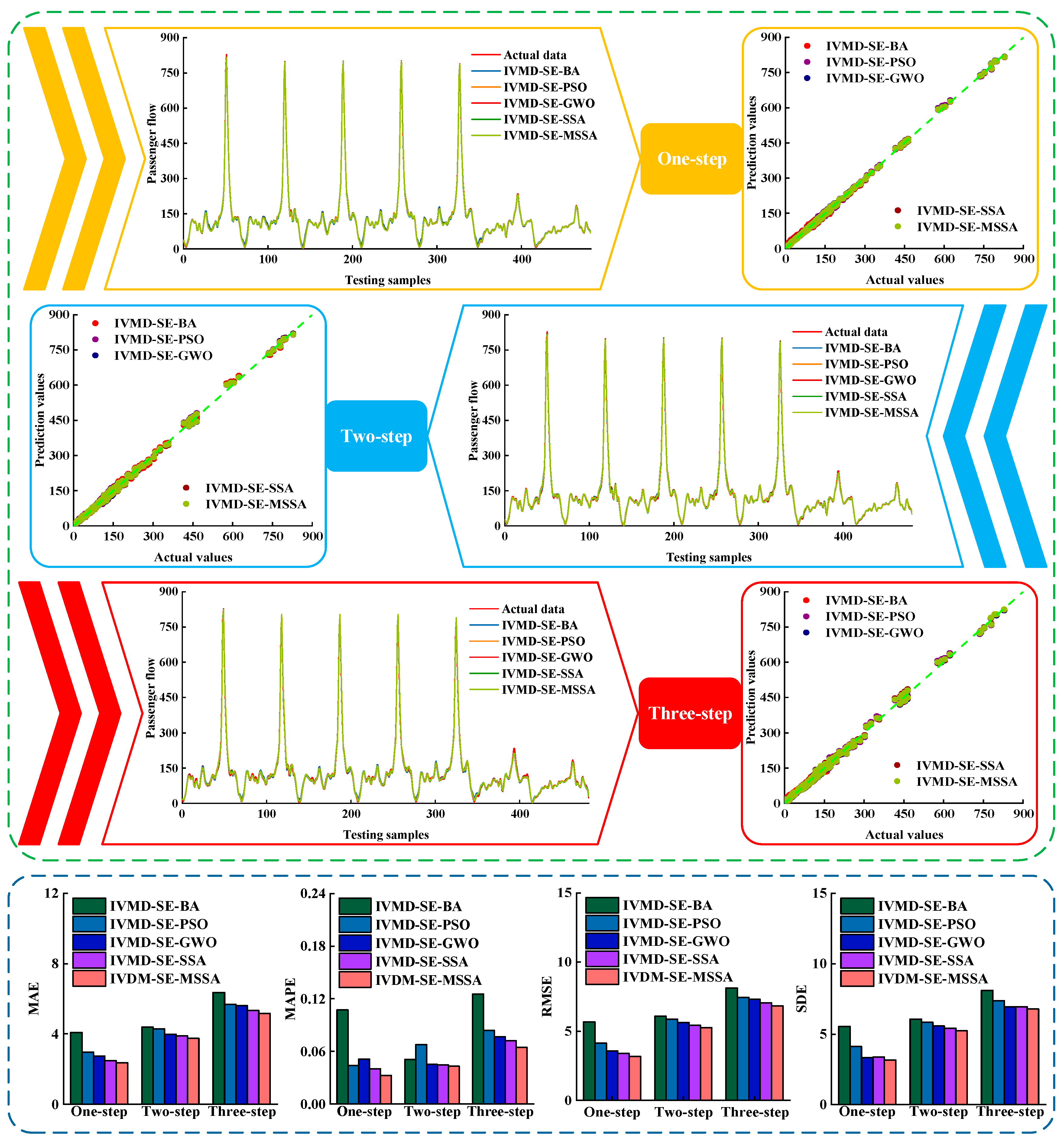
(4) Experiments are carried out on four subway station passenger flow datasets. The experimental results show that IVMD-SE-MSSA has the best prediction accuracy. This method has good applicability for different types of stations.
However, this study also has some limitations. Although IVMD-SE-MSSA has good prediction accuracy, the impact of weather conditions on passenger flow is not explicitly considered in the study. Moreover, although MSSA is used to combine sub-series prediction results, it is essentially a linear combination. How to adopt a better nonlinear combination method while considering the influence of weather is also a problem to be solved in future research.

Author Contributions

Conceptualization and methodology, X.L.; writing—original draft preparation, X.L.; investigation, X.L., Z.H. and S.L.; resources and supervision Z.H. and Y.Z.; data curation, J.W.; project administration, X.L. All authors have read and agreed to the published version of the manuscript.

Funding

This research was funded by Guangxi Key Laboratory of Manufacturing System & Advanced Manufacturing Technology, grant number 19-050-44-S006.

Institutional Review Board Statement

This study does not involve human or animal studies.

Informed Consent Statement

This study does not involve human research.

Data Availability Statement

The authors confirm that the data supporting the findings of this study are available upon request.

Acknowledgments

We thank Guangxi Key Laboratory of Manufacturing Systems and Advanced Manufacturing Technology for supporting this research.

Conflicts of Interest

The authors declare that they have no known competing financial interest or personal relationships that could have appeared to influence the work reported in this paper.

References

  1. Lu, K.; Han, B.M.; Lu, F.; Wang, Z.J. Urban Rail Transit in China: Progress Report and Analysis (2008–2015). Urban Rail Transit 2016, 2, 93–105. [Google Scholar] [CrossRef]
  2. Ma, X.L.; Zhang, J.Y.; Du, B.W.; Ding, C.; Sun, L.L. Parallel Architecture of Convolutional Bi-Directional LSTM Neural Networks for Network-Wide Metro Ridership Prediction. IEEE Trans. Intell. Transp. Syst. 2019, 20, 2278–2288. [Google Scholar] [CrossRef]
  3. Wei, Y.; Chen, M.C. Forecasting the Short-Term Metro Passenger Flow with Empirical Mode Decomposition and Neural Networks. Transp. Res. Part C Emerg. Technol. 2012, 21, 148–162. [Google Scholar] [CrossRef]
  4. Jiao, P.P.; Li, R.M.; Sun, T.; Hou, Z.H.; Ibrahim, A. Three Revised Kalman Filtering Models for Short-Term Rail Transit Passenger Flow Prediction. Math. Probl. Eng. 2016, 2016, 9717582. [Google Scholar] [CrossRef]
  5. Bezuglov, A.; Comert, G. Short-Term Freeway Traffic Parameter Prediction: Application of Grey System Theory Models. Expert. Syst. Appl. 2016, 62, 284–292. [Google Scholar] [CrossRef]
  6. Smith, B.L.; Demetsky, M.J. Traffic Flow Forecasting: Comparison of Modeling Approaches. J. Transp. Eng. 1997, 123, 261–266. [Google Scholar] [CrossRef]
  7. Ding, C.; Duan, J.X.; Zhang, Y.R.; Wu, X.K.; Yu, G.Z. Using an ARIMA-GARCH Modeling Approach to Improve Subway Short-Term Ridership Forecasting Accounting for Dynamic Volatility. IEEE Trans. Intell. Transp. Syst. 2017, 19, 1054–1064. [Google Scholar] [CrossRef]
  8. Milenkovic, M.; Svadlenka, L.; Melichar, V.; Bojovic, N.; Avramovic, Z. SARIMA Modelling Approach for Railway Passenger Flow Forecasting. Transport 2018, 33, 1113–1120. [Google Scholar] [CrossRef]
  9. Yu, B.; Wang, H.Z.; Shan, W.X.; Yao, B.Z. Prediction of Bus Travel Time Using Random Forests Based on Near Neighbors. Comput.-Aided Civ. Inf. 2018, 33, 333–350. [Google Scholar] [CrossRef]
  10. Azeez, O.S.; Pradhan, B.; Shafri, H.Z.M. Vehicular CO Emission Prediction Using Support Vector Regression Model and GIS. Sustainability 2018, 10, 3434. [Google Scholar] [CrossRef]
  11. Qu, W.R.; Li, J.H.; Yang, L.; Li, D.L.; Liu, S.S.; Zhao, Q.; Qi, Y. Short-Term Intersection Traffic Flow Forecasting. Sustainability 2020, 12, 8158. [Google Scholar] [CrossRef]
  12. Roos, J.; Bonnevay, S.; Gavin, G. Dynamic Bayesian Networks with Gaussian Mixture Models for Short-Term Passenger Flow Forecasting. In Proceedings of the 12th International Conference on Intelligent Systems and Knowledge Engineering, Nanjing, China, 24–26 November 2017; pp. 1–8. [Google Scholar]
  13. Chen, C.; Wang, H.; Yuan, F.; Jia, H.Z.; Yao, B.Z. Bus Travel Time Prediction Based on Deep Belief Network with Back-Propagation. Neural. Comput. Appl. 2020, 32, 10435–10449. [Google Scholar] [CrossRef]
  14. Ma, X.L.; Yu, H.Y.; Wang, Y.P.; Wang, Y.H. Large-Scale Transportation Network Congestion Evolution Prediction Using Deep Learning Theory. PLoS ONE 2015, 10, e0119044. [Google Scholar] [CrossRef]
  15. Ma, X.L.; Tao, Z.M.; Wang, Y.H.; Yu, H.Y.; Wang, Y.P. Long Short-Term Memory Neural Network for Traffic Speed Prediction Using Remote Microwave Sensor Data. Transp. Res. Part C Emerg. Technol. 2015, 54, 187–197. [Google Scholar] [CrossRef]
  16. Qiu, B.; Zhao, Y. Research on Improved Traffic Flow Prediction Network Based on CapsNet. Sustainability 2022, 14, 15996. [Google Scholar] [CrossRef]
  17. Xu, Z.J.; Hou, L.Y.; Zhang, Y.Y.; Zhang, J.Q. Passenger Flow Prediction of Scenic Spot Using a GCN-RNN Model. Sustainability 2022, 14, 3295. [Google Scholar] [CrossRef]
  18. Cai, L.R.; Lei, M.Q.; Zhang, S.Y.; Yu, Y.D.; Zhou, T.; Qin, J. A Noise-Immune LSTM Network for Short-Term Traffic Flow Forecasting. Chaos 2020, 30, 023135. [Google Scholar] [CrossRef]
  19. Chen, X.Q.; Lu, J.Q.; Zhao, J.S.; Qu, Z.J.; Yan, Y.S.; Xian, J.F. Traffic Flow Prediction at Varied Time Scales Via Ensemble Empirical Mode Decomposition and Artificial Neural Network. Sustainability 2020, 12, 3678. [Google Scholar] [CrossRef]
  20. Shen, L.; Lu, J.; Geng, D.D.; Deng, L. Peak Traffic Flow Predictions: Exploiting Toll Data from Large Expressway Networks. Sustainability 2021, 13, 260. [Google Scholar] [CrossRef]
  21. Li, Y.P.; Ma, C.X. Short-Time Bus Route Passenger Flow Prediction Based on a Secondary Decomposition Integration Method. J. Transp. Eng. Part A Syst. 2023, 149, 04022132. [Google Scholar] [CrossRef]
  22. Wu, Z.; Huang, N. Ensemble Empirical Mode Decomposition: A Noise-Assisted Data Analysis Method. Adv. Adapt. Data Anal. 2009, 1, 1–41. [Google Scholar] [CrossRef]
  23. Liu, J.; Wu, N.Q.; Qiao, Y.; Li, Z.W. Short-Term Traffic Flow Forecasting Using Ensemble Approach Based on Deep Belief Networks. IEEE Trans. Intell. Transp. Syst. 2022, 23, 404–417. [Google Scholar] [CrossRef]
  24. Cao, Y.; Hou, X.L.; Chen, N. Short-Term Forecast of OD Passenger Flow Based on Ensemble Empirical Mode Decomposition. Sustainability 2022, 14, 8562. [Google Scholar] [CrossRef]
  25. Yeh, J.R.; Shieh, J.S.; Huang, N. Complementary Ensemble Empirical Mode Decomposition: A Novel Noise Enhanced Data Analysis Method. Adv. Adapt. Data Anal. 2010, 2, 135–156. [Google Scholar] [CrossRef]
  26. Jiang, Y.; Han, L.; Gao, Y. Artificial Intelligence-Enabled Smart City Construction. J. Supercomput. 2022, 78, 19501–19521. [Google Scholar] [CrossRef]
  27. Torres, M.E.; Colominas, M.A.; Schlotthauer, G.; Flandrin, P. A Complete Ensemble Empirical Mode Decomposition with Adaptive Noise. In Proceedings of the IEEE International Conference on Acoustics, Speech, and Signal Processing, Prague Congress Ctr, Prague, Czech Republic, 22–27 May 2011; pp. 4144–4147. [Google Scholar]
  28. Li, G.X.; Zhong, X. Parking Demand Forecasting Based on Improved Complete Ensemble Empirical Mode Decomposition and GRU Model. Eng. Appl. Artif. Intell. 2023, 119, 105717. [Google Scholar] [CrossRef]
  29. Huang, H.; Mao, J.N.; Lu, W.K.; Hu, G.J.; Liu, L. DEASeq2Seq: An Attention Based Sequence to Sequence Model for Short-Term Metro Passenger Flow Prediction within Decomposition-Ensemble Strategy. Transp. Res. Part C Emerg. Technol. 2023, 146, 103965. [Google Scholar] [CrossRef]
  30. Huang, H.C.; Chen, J.Y.; Huo, X.T.; Qiao, Y.F.; Ma, L. Effect of Multi-Scale Decomposition on Performance of Neural Networks in Short-Term Traffic Flow Prediction. IEEE Access 2021, 9, 50994–51004. [Google Scholar] [CrossRef]
  31. Sun, Y.X.; Leng, B.; Guan, W. A Novel Wavelet-SVM Short-Time Passenger Flow Prediction in Beijing Subway System. Neurocomputing 2015, 166, 109–121. [Google Scholar] [CrossRef]
  32. Yang, X.; Xue, Q.C.; Yang, X.X.; Yin, H.D.; Qu, Y.C.; Li, X.; Wu, J.J. A Novel Prediction Model for the Inbound Passenger Flow of Urban Rail Transit. Inf. Sci. 2021, 566, 347–363. [Google Scholar] [CrossRef]
  33. Ozger, M.; Basakin, E.E.; Ekmekcioglu, O.; Hacisuleyman, V. Comparison of Wavelet and Empirical Mode Decomposition Hybrid Models in Drought Prediction. Comput. Electron. Agric. 2020, 179, 105851. [Google Scholar] [CrossRef]
  34. Dragomiretskiy, K.; Zosso, D. Variational Mode Decomposition. IEEE Trans. Signal Process. 2014, 62, 531–544. [Google Scholar] [CrossRef]
  35. Sharma, V.; Parey, A. Extraction of Weak Fault Transients Using Variational Mode Decomposition for Fault Diagnosis of Gearbox Under Varying Speed. Eng. Fail. Anal. 2019, 107, 104204. [Google Scholar] [CrossRef]
  36. Zhang, Y.Y.; Zhu, C.F.; Wang, Q.R. LightGBM-Based Model for Metro Passenger Volume Forecasting. IET Intell. Transp. Syst. 2021, 14, 1815–1823. [Google Scholar] [CrossRef]
  37. Zhou, T.Q.; Wu, W.T.; Peng, L.Q.; Zhang, M.Y.; Li, Z.X.; Xiong, Y.B.; Bai, Y.L. Evaluation of Urban Bus Service Reliability on Variable Time Horizons Using a Hybrid Deep Learning Method. Reliab. Eng. Syst. Saf. 2022, 217, 108090. [Google Scholar] [CrossRef]
  38. Rayi, V.K.; Mishra, S.P.; Naik, J.; Dash, P.K. Adaptive VMD Based Optimized Deep Learning Mixed Kernel ELM Autoencoder for Single and Multistep Wind Power Forecasting. Energy 2022, 244, 122585. [Google Scholar] [CrossRef]
  39. Moreno, S.R.; da Silva, R.G.; Mariani, V.C.; Coelho, L.D. Multi-Step Wind Speed Forecasting Based on Hybrid Multi-Stage Decomposition Model and Long Short-Term Memory Neural Network. Energy. Convers. Manag. 2020, 213, 112869. [Google Scholar] [CrossRef]
  40. Wang, J.J.; Chen, Y.; Zhu, S.Z.; Xu, W.J. Depth Feature Extraction-Based Deep Ensemble Learning Framework for High Frequency Futures Price Forecasting. Digit. Signal Process. 2022, 127, 103567. [Google Scholar] [CrossRef]
  41. Shi, F.; Yang, X.Q.; Hu, X.L.; Xu, G.M.; Wu, R.F. A VMD-GA-BP Method for Predicting Non-Holiday Passenger Flow of High Speed Railway Based on Data Replacement Correction. China Railw. Sci. 2019, 40, 129–136. [Google Scholar]
  42. Fu, W.L.; Wang, K.; Li, C.S.; Tan, J.W. Multi-Step Short-Term Wind Speed Forecasting Approach Based on Multi-Scale Dominant Ingredient Chaotic Analysis, Improved Hybrid GWO-SCA Optimization and ELM. Energy Convers. Manag. 2019, 189, 356–377. [Google Scholar] [CrossRef]
  43. Huang, Y.S.; Gao, Y.L.; Gan, Y.; Ye, M. A New Financial Data Forecasting Model Using Genetic Algorithm and Long Short-Term Memory Network. Neurocomputing 2021, 425, 207–218. [Google Scholar] [CrossRef]
  44. Liu, Q.; Liu, M.; Zhou, H.L.; Yan, F. A Multi-Model Fusion Based Non-Ferrous Metal Price Forecasting. Resour. Policy 2022, 77, 102714. [Google Scholar] [CrossRef]
  45. Li, G.H.; Zheng, C.F.; Yang, H. Carbon Price Combination Prediction Model Based on Improved Variational Mode Decomposition. Energy Rep. 2022, 8, 1644–1664. [Google Scholar] [CrossRef]
  46. Yang, K.; Wang, B.F.; Qiu, X.; Li, J.H.; Wang, Y.Z.; Liu, Y.L. Multi-Step Short-Term Wind Speed Prediction Models Based on Adaptive Robust Decomposition Coupled with Deep Gated Recurrent Unit. Energies 2022, 15, 4221. [Google Scholar] [CrossRef]
  47. Xue, J.K.; Shen, B. A novel Swarm Intelligence Optimization Approach: Sparrow Search Algorithm. Syst. Sci. Control. Eng. 2020, 8, 22–34. [Google Scholar] [CrossRef]
  48. Song, J.M.; Li, S.P. Elite Opposition Learning and Exponential Function Steps-Based Dragonfly Algorithm for Global Optimization. In Proceedings of the 2017 IEEE International Conference on Information and Automation, Macau, China, 18–20 July 2017; pp. 1178–1183. [Google Scholar]
  49. Arora, S.; Singh, S. Butterfly Optimization Algorithm: A Novel Approach for Global Optimization. Soft Comput. 2019, 23, 715–734. [Google Scholar] [CrossRef]
  50. Zhou, F.J.; Wang, X.J.; Zhang, M. Evolutionary Programming Using Mutations Based on the T Probability Distribution. Acta Electron. Sin. 2008, 36, 667–671. [Google Scholar]
  51. Duan, J.d.; Peng, W.; Ma, W.T.; Shuai, F.; Hou, Z.Q. A Novel Hybrid Model Based on Nonlinear Weighted Combination for Short-Term Wind Power Forecasting. Int. J. Electr. Power Energy Syst. 2022, 134, 107452. [Google Scholar] [CrossRef]
  52. Liu, H.; Zhang, X.Y. AQI Time Series Prediction Based on a Hybrid Data Decomposition and Echo State Networks. Environ. Sci. Pollut. Res. 2021, 28, 51160–51182. [Google Scholar] [CrossRef]
  53. Li, H.T.; Jin, F.; Sun, S.L.; Li, Y.W. A New Secondary Decomposition Ensemble Learning Approach for Carbon Price Forecasting. Knowl. Based Syst. 2021, 214, 106686. [Google Scholar] [CrossRef]
  54. Jin, Z.Z.; He, D.Q.; Ma, R.; Zou, X.Y.; Chen, Y.J.; Shan, S. Fault Diagnosis of Train Rotating Parts Based on Multi-Objective VMD Optimization and Ensemble Learning. Digit. Signal Process. 2022, 121, 103312. [Google Scholar] [CrossRef]
  55. Gai, J.B.; Shen, J.X.; Hu, Y.F.; Wang, H. An Integrated Method Based on Hybrid Grey Wolf Optimizer Improved Variational Mode Decomposition and Deep Neural Network for Fault Diagnosis of Rolling Bearing. Measurement 2020, 162, 107901. [Google Scholar] [CrossRef]
  56. Xie, B.L.; Sun, Y.; Huang, X.L.; Yu, L.; Xu, G.Y. Travel Characteristics Analysis and Passenger Flow Prediction of Intercity Shuttles in the Pearl River Delta on Holidays. Sustainability 2020, 12, 7249. [Google Scholar] [CrossRef]
  57. Hochreiter, S.; Schmidhuber, J. Long Short-Term Memory. Neural. Comput. 1997, 9, 1735–1780. [Google Scholar] [CrossRef]
  58. Luong, M.T.; Pham, H.; Manning, C.D. Effective Approaches to Attention-Based Neural Machine Translation. arXiv 2015, arXiv:1508.04025. [Google Scholar]
  59. Bontempi, G.; Ben Taieb, S. Conditionally Dependent Strategies for Multiple-Step-Ahead Prediction in Local Learning. Int. J. Forecast. 2011, 27, 689–699. [Google Scholar] [CrossRef]
  60. Bontempi, G. Long Term Time Series Prediction with Multi-Input Multi-Output Local Learning. In Proceedings of the 2nd European Symposium on Time Series Prediction (TSP), Helsinki, Finland; 2008; pp. 145–154. Available online: https://citeseerx.ist.psu.edu/document?repid=rep1&type=pdf&doi=c28782ed6d0be1d29f98c9018462d3eafac4d558 (accessed on 24 March 2023).
  61. Zsuzsa, P.; Radu-Emil, P.; Tar, J.K.; Marta, T. Use of Multi-parametric Quadratic Programming in Fuzzy Control Systems. Acta Polytech. Hung. 2006, 3, 29. [Google Scholar]
  62. Precup, R.E.; David, R.C.; Roman, R.C.; Petriu, E.M.; Szedlak-Stinean, A.I. Slime Mould Algorithm-Based Tuning of Cost-Effective Fuzzy Controllers for Servo Systems. Int. J. Comput. Intell. Syst. 2021, 14, 1042–1052. [Google Scholar] [CrossRef]
  63. Sawulski, J.; Lawrynczuk, M. Optimization of Control Strategy for A Low Fuel Consumption Vehicle Engine. Inf. Sci. 2019, 493, 192–216. [Google Scholar] [CrossRef]
  64. Yang, X.S. A New Metaheuristic Bat-Inspired Algorithm. In Proceedings of the International Workshop on Nature Inspired Cooperative Strategies for Optimization, Tenerife, Spain. 2008, pp. 65–74. Available online: https://link.springer.com/book/10.1007/978-3-642-03211-0 (accessed on 24 March 2023).
  65. Chen, J.; Liu, H.; Chen, C.; Duan, Z. Wind Speed Forecasting Using Multi-Scale Feature Adaptive Extraction Ensemble Model with Error Regression Correction. Expert. Syst. Appl. 2022, 207, 117358. [Google Scholar] [CrossRef]
Figure 1. Basic structure of the LSTM network.
Sustainability 15 07949 g001
Figure 2. The attention mechanism.
Sustainability 15 07949 g002
Figure 3. The process of the proposed short-term passenger flow prediction model.
Sustainability 15 07949 g003
Figure 4. Four original station passenger flow datasets.
Sustainability 15 07949 g004
Figure 5. Comparison of convergence curves of each optimization algorithm.
Sustainability 15 07949 g005
Figure 6. Comparison of convergence curves of VMD optimized by each algorithm.
Sustainability 15 07949 g006
Figure 7. Decomposition results of IVMD on station 1.
Sustainability 15 07949 g007
Figure 8. Decomposition results of IVMD on station 2.
Sustainability 15 07949 g008
Figure 9. Decomposition results of IVMD on station 3.
Sustainability 15 07949 g009
Figure 10. Decomposition results of IVMD on station 4.
Sustainability 15 07949 g010
Figure 11. The SE calculation results for each IMF component of four station datasets.
Sustainability 15 07949 g011
Figure 12. Comparison of multi-step prediction performance of each model in experiment 1 at station 1.
Sustainability 15 07949 g012
Figure 13. Comparison of multi-step prediction performance of each model in experiment 2 at station 2.
Sustainability 15 07949 g013
Figure 14. Comparison of multi-step prediction performance of different data preprocessing techniques in experiment 3 at station 3.
Sustainability 15 07949 g014
Figure 15. Comparison of multi-step prediction performance of each models inexperiment 4 at station 4.
Sustainability 15 07949 g015
Table 1. Characteristics of passenger flow datasets of four stations.
AreaDatasetsNumbersMeanStdMaxMin
Passenger/15 minPassenger/15 minPassenger/15 minPassenger/15 min
Station 1All Samples193249731718921
Training144948731518921
Testing48352932115051
Station 2All Samples193229017711031
Training144927016011031
Testing4833512109451
Station 3All Samples19322691337522
Training14492541257522
Testing4833111506833
Station 4All Samples19321371358591
Training14491371378591
Testing4831351278282
Table 2. Benchmark test functions.
FunctionDimRange
F 1 ( x ) = i = 1 n x i + i = 1 n x i 30[−100, 100]
F 2 ( x ) = 1 + 1 4000 i = 1 n x i 2 i = 1 n cos ( x i i ) 30[−600, 600]
F 3 ( x ) = 20 + e 20 exp ( 0.2 1 n i = 1 n x i 2 ) exp [ 1 n i = 1 n cos ( 2 π x i ) ] 30[−32, 32]
F 4 ( x ) = i = 1 n [ x i 2 10 cos ( 2 π x i ) + 10 ] + 10 d 30[−5.12, 5.12]
Table 3. Parameter settings of the optimization algorithm.
AlgorithmParameter Settings
SSASame as the ISSA algorithm.
GWOThe convergence factor a = 2 t ( 2 / i t e r max ) , r1 and r2 are random values between 0 and 1.
PSOThe inertia weight w is 0.6, learning factor c1 = c2 = 2, r1 and r2 are random values between 0 and 1.
BAThe loudness is set to 0.5, the pulse rate is set to 0.5, and the maximum and minimum frequencies are 2 and 0, respectively.
Table 4. VMD parameters of four stations generated by MSSA algorithm.
DatasetsParameters
kα
Chaoyang Square Station14229
Nanning East Railway Station15261
Nanning Railway Station1528
Jinhu Square Station1344
Table 5. Comparison of prediction performance between IVMD-SE-MSSA and single models.
DatasetsModelOne-StepTwo-StepThree-Step
MAEMAPERMSESDEMAEMAPERMSESDEMAEMAPERMSESDE
Station 1BP27.65460.873437.756137.75461.11381.165589.924289.858287.13822.4289131.1663131.1583
LSTM24.57660.735833.142631.634451.18830.805677.643776.129676.94061.2357119.2811117.2727
ALSTM22.18110.654529.748329.667850.23350.713373.695673.368774.93351.1901113.3697113.3469
IVMD-SE-MSSA3.6770.03284.66344.06175.76970.03977.70137.6998.18810.051910.889810.8884
Station 2BP32.22021.326244.884644.839777.27775.9772107.9911106.809499.98319.3231137.2924137.3857
LSTM30.53841.295342.298742.722968.9553.2528102.9544102.583895.97776.8783134.9631134.7885
ALSTM28.92390.7740.004740.224665.27832.647299.304899.818993.57334.9698130.038130.7334
IVMD-SE-MSSA2.68220.07343.47763.47294.69140.06986.23046.22097.8480.222110.693810.6887
Station 3BP27.25710.244234.926234.880163.00220.563982.605382.394286.39950.758109.4136108.3756
LSTM24.6570.194433.603632.946754.24490.321475.397874.732175.5310.5808103.3296101.262
ALSTM23.1590.14631.964531.962654.11190.294974.645473.293572.95040.527299.423696.3957
IVMD-SE-MSSA1.56460.011.96261.96263.72270.02254.6594.65826.48350.04177.94447.9443
Station 4BP15.61060.161420.113220.219724.9890.252943.58443.154342.06550.430569.626369.301
LSTM14.03350.141419.658418.678223.48730.234641.837640.428933.32660.354466.936566.5205
ALSTM9.58880.098215.578115.547222.74520.218540.472440.368232.4460.330165.690765.0133
IVMD-SE-MSSA2.3470.03253.16463.16233.74770.0435.24965.24715.16480.06466.82616.7915
Table 6. Comparison of prediction performance of different prediction models after using IVMD.
DatasetsModelOne-StepTwo-StepThree-Step
MAEMAPERMSESDEMAEMAPERMSESDEMAEMAPERMSESDE
Station 1IVMD-BP6.88480.05098.64838.16467.98750.05599.79468.524412.27440.084115.545915.5284
IVMD-ALSTM10.61550.060318.710617.117611.19980.067919.084218.627613.23240.085420.776820.6281
IVMD-SE4.73710.04876.08146.08097.21240.04598.76148.522410.28750.077913.339612.8593
IVMD-SE-MSSA3.6770.03284.66344.06175.76970.03977.70137.6998.18810.051910.889810.8884
Station 2IVMD-BP14.91940.459822.572622.571215.36030.373522.875822.872116.47450.403123.725123.7185
IVMD-ALSTM24.5090.500934.747134.69824.76510.424735.73435.689225.69120.462736.163736.11
IVMD-SE5.31230.32536.30664.08376.47420.21088.11626.55019.54970.354212.272811.313
IVMD-SE-MSSA2.68220.07343.47763.47294.69140.06986.23046.22097.8480.222110.693810.6887
Station 3IVMD-BP3.71250.03755.83815.83694.21030.04036.18126.18079.07220.05149.29489.6261
IVMD-ALSTM8.50390.05310.739510.73838.97260.054611.43211.430710.05110.061612.726912.7258
IVMD-SE2.36590.01212.97252.80425.56240.0386.95656.02475.48390.05077.67717.677
IVMD-SE-MSSA1.56460.011.96261.96263.72270.02254.6594.65826.48350.04177.94447.9443
Station 4IVMD-BP3.42410.03655.53654.96674.75910.04987.34897.31147.23110.07489.70068.9286
IVMD-ALSTM3.68430.0455.59355.15257.51290.074511.897211.274710.27790.169116.884716.8558
IVMD-SE3.20650.03385.31725.12094.68190.04717.33567.25387.03470.07489.62868.9105
IVMD-SE-MSSA2.3470.03253.16463.16233.74770.0435.24965.24715.16480.06466.82616.7915
Table 7. Comparison of prediction performance of different data preprocessing techniques hybrid models.
DatasetsModelOne-StepTwo-StepThree-Step
MAEMAPERMSESDEMAEMAPERMSESDEMAEMAPERMSESDE
Station 1EMD-SE-MSSA12.26020.249916.200316.199424.10570.426732.773332.7734.26020.474145.655845.6496
EEMD-SE-MSSA11.02630.234514.88714.886517.4760.336824.330824.330327.29320.446739.446339.4459
CEEMDAN-SE-MSSA14.30150.253820.623320.61927.6110.44440.044940.044137.0360.722151.892351.8911
WD-SE-MSSA8.28630.060411.087710.961513.91810.319518.47718.411517.11470.414922.098422.0447
IVMD-SE-MSSA3.6770.03284.66344.06175.76970.03977.70137.6998.18810.051910.889810.8884
Station 2EMD-SE-MSSA26.55250.693738.734438.728335.7370.92550.751950.750142.25621.6658.198758.1962
EEMD-SE-MSSA17.62250.332326.788726.771324.1160.548235.27335.270635.04260.97650.43750.426
CEEMDAN-SE-MSSA17.83990.579924.775424.767929.6280.776641.681141.67940.4951.47856.044356.0418
WD-SE-MSSA14.910.212124.116624.031222.20910.427331.148731.121721.98170.850931.700131.6977
IVMD-SE-MSSA2.68220.07343.47763.47294.69140.06986.23046.22097.8480.222110.693810.6887
Station 3EMD-SE-MSSA19.41010.12728.00928.00734.51380.180548.820948.819342.98730.239558.193658.1931
EEMD-SE-MSSA9.72870.06913.54613.537915.47280.097921.097521.097424.99140.176732.753932.7534
CEEMDAN-SE-MSSA25.41290.15836.191436.191337.92620.20654.157554.157143.89990.230461.129461.1283
WD-SE-MSSA7.67120.058511.139611.139113.50750.087717.906917.906313.36390.092817.3517.3492
IVMD-SE-MSSA1.56460.011.96261.96263.72270.02254.6594.65826.48350.04177.94447.9443
Station 4EMD-SE-MSSA7.26070.090411.455511.455416.9480.189529.930329.9321.88990.252735.142735.142
EEMD-SE-MSSA5.13740.07617.51257.51217.34880.11089.82919.823110.69420.124216.639416.9331
CEEMDAN-SE-MSSA7.59580.085612.6512.649317.06560.186431.957531.956222.45470.246439.724939.7248
WD-SE-MSSA3.38220.04944.45244.37656.64330.08469.33929.29668.49730.110411.061710.973
IVMD-SE-MSSA2.3470.03253.16463.16233.74770.0435.24965.24715.16480.06466.82616.7915
Table 8. Comparison of prediction performance proposed model and combined models using different optimization algorithms.
DatasetsModelOne-StepTwo-StepThree-Step
MAEMAPERMSESDEMAEMAPERMSESDEMAEMAPERMSESDE
Station 1IVMD-SE-BA9.7240.232313.2613.255111.27870.130414.591714.591612.74190.154816.135716.13
IVMD-SE-PSO6.14090.18468.8978.89648.41540.069210.899210.898910.08660.139512.977912.9778
IVMD-SE-GWO5.05270.04717.16636.49546.18340.04728.09758.01099.22450.067111.846111.346
IVMD-SE-SSA4.85110.04076.32116.31955.93020.04057.91297.91238.51370.055411.272411.2717
IVMD-SE-MSSA3.6770.03284.66344.06175.76970.03977.70137.6998.18810.051910.889810.8884
Station 2IVMD-SE-BA6.30930.21487.77977.75847.51940.20859.62689.583610.59420.52413.987413.9828
IVMD-SE-PSO5.20160.20046.07216.60096.72380.16198.74028.73419.13160.378612.091712.081
IVMD-SE-GWO4.26440.16845.68775.67866.44310.12897.92026.3119.04570.354811.775510.8409
IVMD-SE-SSA2.78540.10183.62333.61734.79020.08626.32346.2347.98930.270510.843210.7362
IVMD-SE-MSSA2.68220.07343.47763.47294.69140.06986.23046.22097.8480.222110.693810.6887
Station 3IVMD-SE-BA3.65120.02174.5514.55096.12660.03577.47117.47049.00110.056310.899510.8957
IVMD-SE-PSO2.76220.01853.42493.42485.55220.03476.98836.98818.21090.04939.99039.9901
IVMD-SE-GWO1.93840.01472.35672.10435.11370.036.00044.75869.41350.05111.26868.198
IVMD-SE-SSA1.75880.01082.18862.18843.96080.0244.87944.87796.70370.04298.14248.1422
IVMD-SE-MSSA1.56460.011.96261.96263.72270.02254.6594.65826.48350.04177.94447.9443
Station 4IVMD-SE-BA4.08630.10735.65845.54694.38090.05086.07886.0716.3580.12548.11778.1176
IVMD-SE-PSO2.9580.04394.12644.12614.27730.06775.85125.84945.68160.08387.43767.3873
IVMD-SE-GWO2.73930.0513.56823.33043.97880.04515.61595.5885.61390.07657.29666.9438
IVMD-SE-SSA2.47380.04013.37983.37363.88670.04465.43465.42985.33850.07227.03516.9563
IVMD-SE-MSSA2.3470.03253.16463.16233.74770.0435.24965.24715.16480.06466.82616.7915
Table 9. Four improvement percentages of criteria adopted to discuss prediction performance.
MetricDefinitionEquation
PMAEImprovement percentages of MAE. P M A E = M A E 1 M A E 2 M A E 2 × 100 %
PMAPEImprovement percentages of MAPE. P M A P E = M A P E 1 M A P E 2 M A P E 2 × 100 %
PRMSEImprovement percentages of RMSE. P R M S E = R M S E 1 R M S E 2 R M S E 2 × 100 %
PSDEImprovement percentages of SDE. P S D E = S D E 1 S D E 2 S D E 2 × 100 %
Table 10. Improvement percentages of proposed model compared with each related model.
ModelStation 1Station 2Station 3Station 4
PMAEPMAPEPRMSEPSDEPMAEPMAPEPRMSEPSDEPMAEPMAPEPRMSEPSDEPMAEPMAPEPRMSEPSDE
BP89.9797.2291.0291.2592.7397.892.9792.9593.3495.2693.5893.5586.3883.4288.5788.54
LSTM88.4595.5289.8989.9492.2196.892.7292.7292.3893.2393.1493.0384.1180.8288.1387.9
ALSTM88.0395.1489.2789.5391.8995.6492.4392.4792.1692.3492.9392.7882.6278.3487.4887.43
IVMD-BP35.0434.8331.5829.767.4470.4570.5170.5330.7442.5731.6632.7126.9513.0432.5228.32
IVMD-ALSTM49.6841.7660.359.8279.773.6980.8780.8657.2456.1558.2658.2647.5751.4655.6754.33
IVMD-SE20.727.8817.4917.5328.6658.9723.587.1312.2426.3917.2711.7624.5510.0231.628.58
EMD-SE-MSSA75.0389.1975.4376.0685.4488.8686.1986.287.8586.4489.2189.2175.5873.780.0980.14
EEMD-SE-MSSA68.3987.7870.4471.2180.1880.3281.8681.8876.5578.4178.3978.3951.4354.9755.1555.64
CEEMDAN-SE-MSSA77.6691.2479.3479.8882.787.1183.3583.3689.0287.5290.3890.3876.172.9781.9381.97
WD-SE-MSSA55.1584.3554.9955.9574.2475.4976.5476.5365.9268.9568.6168.6139.2142.6838.6838.32
IVMD-SE-BA47.7475.9647.1348.537.6761.4435.0134.9337.3234.7436.4536.4424.0550.5823.2422.98
IVMD-SE-PSO28.4468.3729.0530.8927.7150.724.1725.6528.7727.6128.6128.6112.8328.312.4912.45
IVMD-SE-GWO13.8122.9214.2212.3922.9443.9819.6310.7228.5122.4725.783.298.718.837.534.17
IVMD-SE-SSA8.68.938.8311.192.2120.331.870.995.254.54.244.233.7610.713.843.55
Table 11. Diebold-Mariano test results.
ModelStation 1Station 2Station 3Station 4
1-Step2-Step3-Step1-Step2-Step3-Step1-Step2-Step3-Step1-Step2-Step3-Step
BP10.895 *8.753 *9.18 *9.818 *10.025 *11.054 *13.95 *12.797 *15.681 *7.285 *5.326 *6.281 *
LSTM9.516 *6.786 *7.616 *8.358 *9.179 *10.286 *10.96 *11.668 *12.057 *8.112 *4.199 *3.609 *
ALSTM11.542 *8.122 *7.837 *9.508 *9.319 *9.648 *11.722 *10.728 *11.303 *6.961 *3.357 *3.523 *
IVMD-BP10.731 *9.412 *10.058 *8.841 *8.489 *8.243 *5.344 *2.983 *11.053 *4.975 *5.168 *6.451 *
IVMD-ALSTM5.93 *5.53 *5.689 *8.191 *7.791 *8.022 *13.934 *12.285 *9.144 *5.393 *5.809 *5.72 *
IVMD-SE5.247 *3.445 *4.919 *12.26 *7.642 *5.56 *10.194 *10.259 *3.645 *4.497 *4.658 *5.936 *
EMD-SE-MSSA11.548 *10.353 *9.948 *8.053 *10.265 *10.976 *6.731 *8.851 *9.908 *5.181 *4.363 *5.853 *
EEMD-SE-MSSA9.991 *9.941 *8.601 *5.662 *7.41 *9.455 *10.498 *9.967 *11.951 *5.405 *7.586 *4.985 *
CEEMDAN-SE-MSSA7.97 *8.956 *8.572 *9.974 *9.883 *10.764 *8.376 *8.552 *9.937 *3.987 *3.202 *4.046 *
WD-SE-MSSA6.246 *8.857 *10.077 *7.807 *10.308 *8.777 *6.499 *10.782 *9.229 *5.319 *6.41 *7.759 *
IVMD-SE-BA10.016 *10.716 *9.672 *13.543 *9.413 *7.434 *12.862 *11.292 *9.244 *10.069 *3.968 *6.578 *
IVMD-SE-PSO6.29 *7.926 *6.169 *13.204 *8.573 *5.136 *11.006 *9.611 *7.953 *5.828 *4.29 *3.444 *
IVMD-SE-GWO6.381 *2.98 *4.552 *7.921 *7.954 *4.848 *7.203 *9.22 *10.695 *5.772 *3.667 *3.756 *
IVMD-SE-SSA5.941 *2.258 **3.044 *2.537 **1.97 **1.495 ***4.976 *3.45 *2.574 **3.497 *2.216 **1.801 ***
Note: * indicates the 1% significance level, ** indicates the 5% significance level, and *** indicates the 10% significance.
Disclaimer/Publisher’s Note: The statements, opinions and data contained in all publications are solely those of the individual author(s) and contributor(s) and not of MDPI and/or the editor(s). MDPI and/or the editor(s) disclaim responsibility for any injury to people or property resulting from any ideas, methods, instructions or products referred to in the content.

