Article

Thermal Transfer Analysis for Sports Footwear, for Performance Athletes, during Volleyball Training

by
Paul Florian Dragoș
1,*,
Marius Darius Șuteu
2,*,
Rareș Pancu
3 and
Sorin Dacian Buhaș
1
1
Department of Physical Education, Sport and Physical Therapy, Faculty of Geography, Tourism and Sport, 1st University Street, 410087 Oradea, Romania
2
Department of Textiles-Leather and Industrial Management, Faculty of Energy Engineering and Industrial Management, University of Oradea, 1st University Street, 410087 Oradea, Romania
3
Department of Engineering and Management, Faculty of Management and Technological Engineering, University of Oradea, 1st University Street, 410087 Oradea, Romania
*
Authors to whom correspondence should be addressed.
Sustainability 2023, 15(1), 652; https://doi.org/10.3390/su15010652
Submission received: 20 November 2022 / Revised: 20 December 2022 / Accepted: 24 December 2022 / Published: 30 December 2022

Abstract

:
The purpose of this paper is a social one, to present various experimental thermal analyses of sports footwear to identify the areas that ensure the best foot ventilation for comfort in movement. The mechanical properties of the analyzed footwear were determined on the Nano Indenter Agilent G200, with the help of which Young’s modulus was determined according to ISO 14577. Thermography measurements were performed at the Oradea University Sports Club. The FLIR SC 640 thermal imaging camera was used, which is a portable thermographic scanning equipment. The measurements were performed on eight athletes (subjects) in a volleyball training session, wearing sports footwear (Asics and Mizuno). Thermographic recordings were made during training at five different times: moment zero (before the start of training), moment one (2 min of training), moment two (5 min of training), moment three (15 min of training), and moment four (at the end of the volleyball training session). For the other three subjects, although having different models of the same sports footwear, the analysis of the thermal distribution values shows they are within the minimum and maximum limits of the five subjects analyzed in the paper. Based on the thermographic recording values obtained, a mathematical model was determined using polynomial regression to predict temperature values outside the range of the experimental data. In the present paper, research was carried out in order to identify the thermal variations of indoor sports shoes used in volleyball training so as to detect the heat exchange between the foot and the outdoor environment. Whether we are talking about winter sports or sports that take place in other atmospheric conditions, the comfort given by the optimal temperature at the level of each body segment is certainly reflected in the level of performance achieved.

1. Introduction

The growing concern of consumers about the comfort of footwear has motivated manufacturers to design footwear with optimal thermal comfort [1,2].
Although the legs represent only 7% of the body surface [3], their exposure to extreme environments can cause discomfort, fatigue, and decreased performance [4,5].
Many of the problems that arise in the foot are directly related to footwear, so it is very important to choose the right footwear [6,7,8].
Regarding the scientific studies based on thermography, a series of papers has been published that analyzes various important aspects regarding heat transfer; this research was conducted with the help of the infrared thermal imaging camera [9,10,11,12].
There is not much research on how, when, and where sports footwear are heated during sports training; there are only a few results regarding the fact that shoe temperatures can rise up to 50 °C during exercise in the summer [13], and the temperature of the footwear must be maintained between 27 °C and 30 °C for optimal thermal comfort [14]. An extreme microclimate inside the footwear contributes to discomfort during wear and decreased performance [15].
In sports, and especially in elite sports, these aspects can have significant effects on the performance obtained by athletes; in their involvement in training and competitions, the superior comfort offered by a quality product is a favorable premise for the aforementioned aspects [16,17,18,19].
The shape of the foot can also affect the comfort degree of the footwear, with high levels of friction in some parts that can lead to increased discomfort due to rising temperatures at the points of contact, with a direct effect on the skin and wounds that may occur at this level. Thus, the structure of the footwear can be brought into discussion, along with its assembly, how foot ventilation is attained, but also the quality of the materials used in the manufacturing process.
Depending on the specific characteristics of the diversity of indoor sports disciplines [20,21,22], the footwear is adapted according to the type of sport practiced; in this case, the athletic setting is volleyball training [23,24,25,26,27,28,29]. In view of this, there are specialized and renowned companies for the manufacture of indoor volleyball footwear that do studies and research in this direction [30,31,32,33].
Lately, however, more and more sports equipment manufacturers who were well-known and recognized for being familiar with a particular sport have begun to diversify in several directions (handball, football, volleyball, fashion, etc.).
Hummel, Mikasa, Craft, Kempa, Nike, New Balance, and Armani are just a few companies that strengthen the idea mentioned above.
In this sense, this study aims to analyze the way and establish the extent to which heat transfers between the foot and the external environment during the training of athletes who practice volleyball, equipped with some models of sports shoes produced for the details of this sport and used by a large majority of players.
The research hypothesis is in line with this goal and seeks to clarify to some extent the influence of materials used in shoe manufacturing on the comfort of athletes, with a direct effect on the level of performance achieved in training and competitions.

2. Materials and Methods

Experimental Research on Footwear Temperature

The infrared thermography examination method [34,35,36] has recently entered the practice of non-destructive examinations, being a method of measuring the thermal field by recording infrared radiation and visualizing the temperature distribution on the observed surfaces [37,38,39].
Thermography measurements were performed at the University Sports Club in Oradea. The FLIR SC 640 thermal imaging camera was used, which is a piece of portable thermographic scanning equipment, ”without cooling”, which has the strongest existing IR detector, with a resolution of 640 × 480 pixels and with a thermal sensitivity encountered so far only by cameras with cooling systems (<0.04 °C).
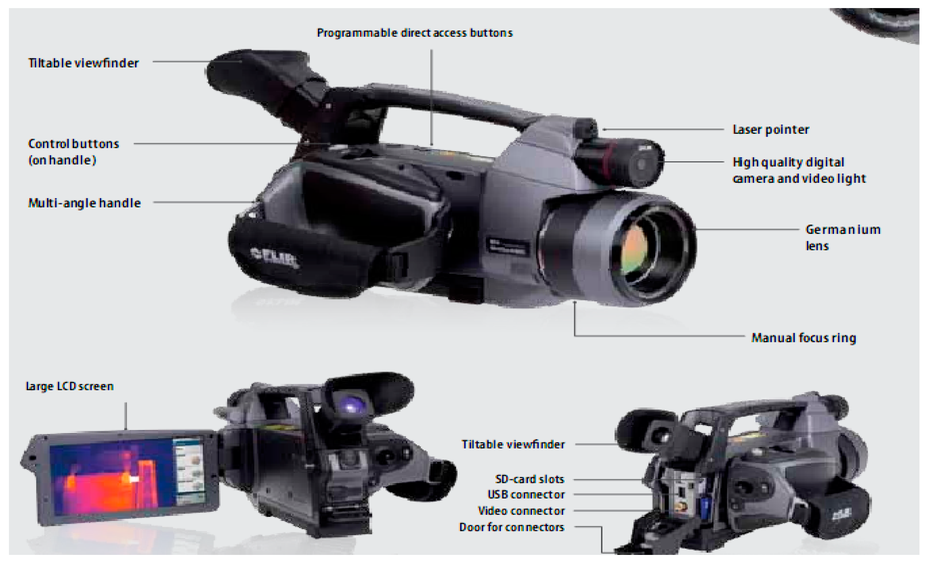
As can be seen from Figure 1, the thermal imaging camera is equipped with a laser pointer, germanium lens, SD card, USB, and video connector.
A great advantage of the FLIR SC 640 thermal imaging camera is that it allows scanning objects remotely, with no contact, the testing being non-destructive for the objects to be measured; it ensures predictive maintenance of equipment and the detection of defects in the early stages to reduce costs. FLIR RESEARCH IR MAX 4.40 software is used for research and development, allowing real-time analysis of the video sequence.
It is well-known that research in the field has led to the emergence of new materials used in sports, footwear with higher elasticity, and optimal forms of footwear that offer customized aerodynamic heel sock lining for the best possible pressure distribution and the insertion of attractive colors, to induce different emotional states, using knowledge of chromotherapy [40,41].
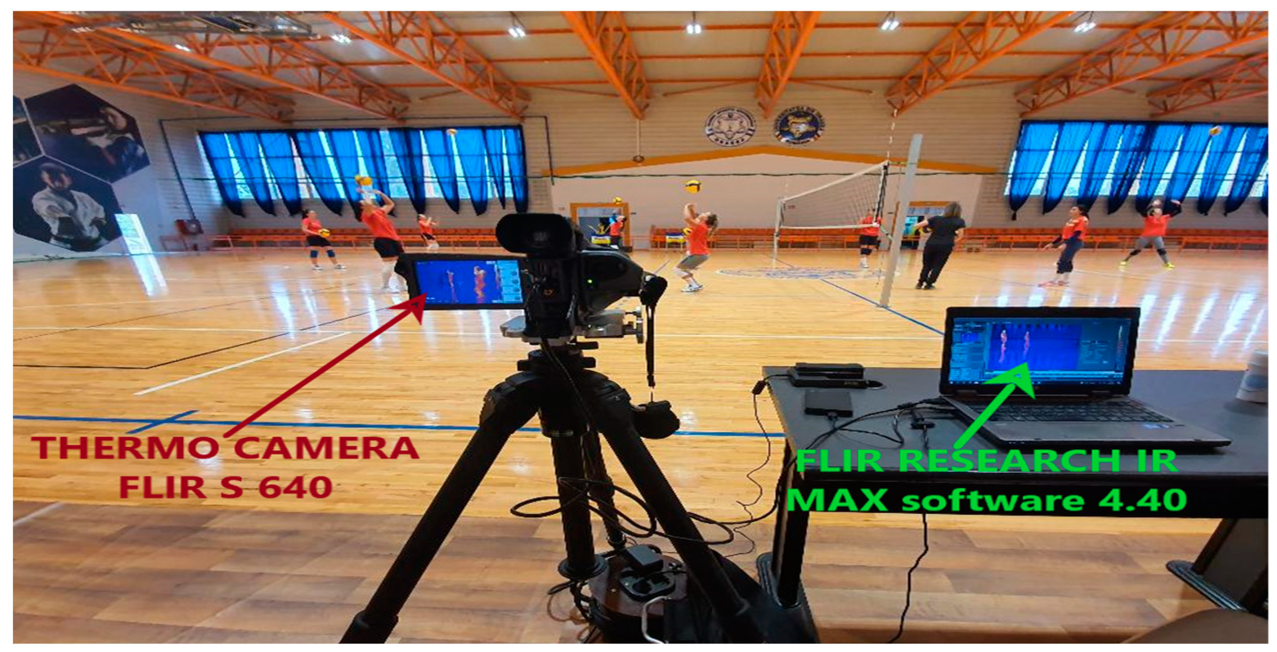
Thermal analysis of sports footwear was performed on 8 subjects during volleyball training, as shown in Figure 2.
In this paper the data for the 5 subjects presented are relevant because they represent the values of the minimum and maximum thermal distribution in the 2 types of sports footwear (Asics and Mizuno) chosen as the most representative of the 8 subjects analyzed participating in volleyball training.
Analysis of the other 3 subjects, although having different models of the same sports footwear, shows that the thermal distribution values are within the minimum and maximum limits of the 5 subjects analyzed in the paper.
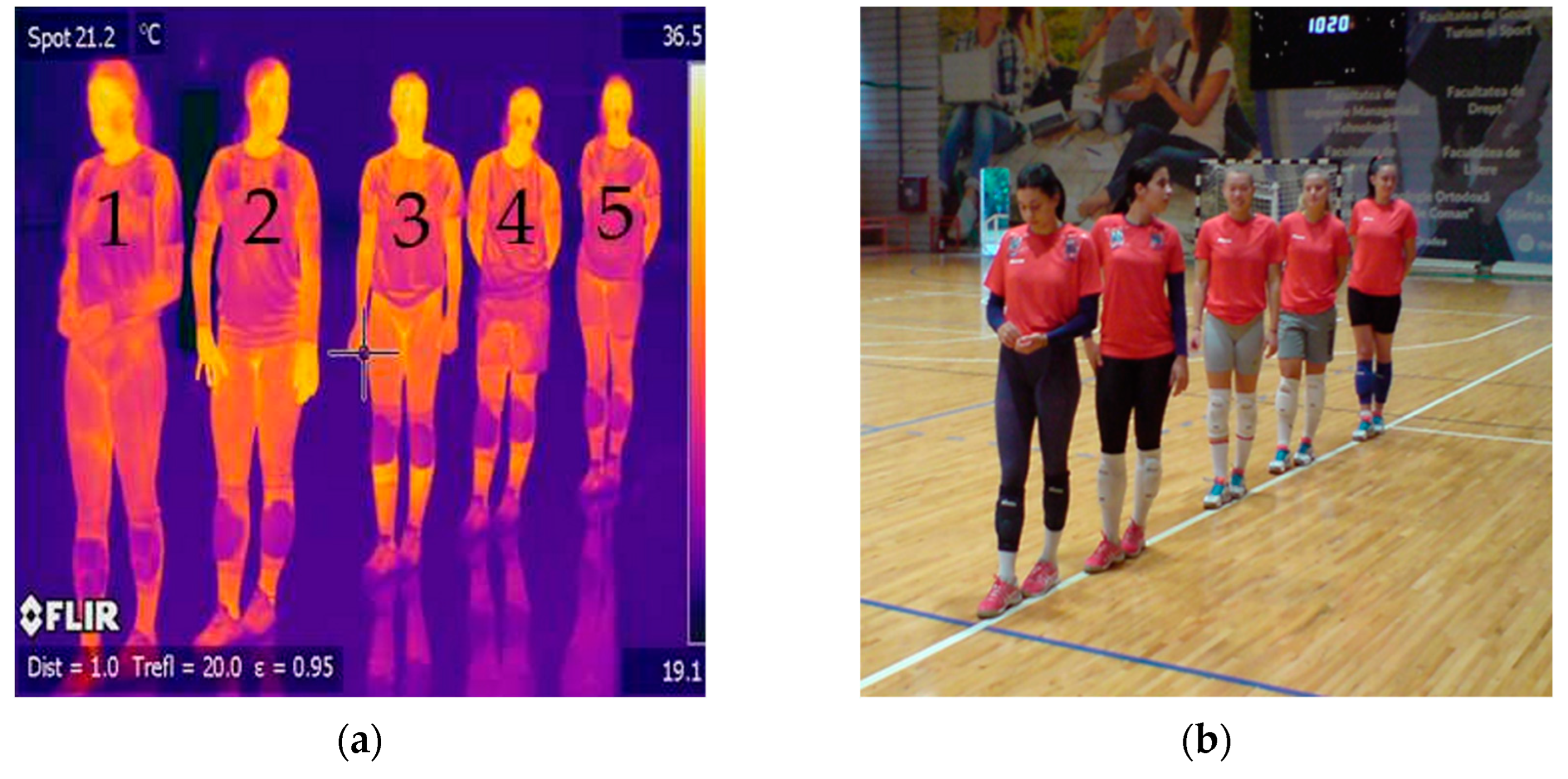
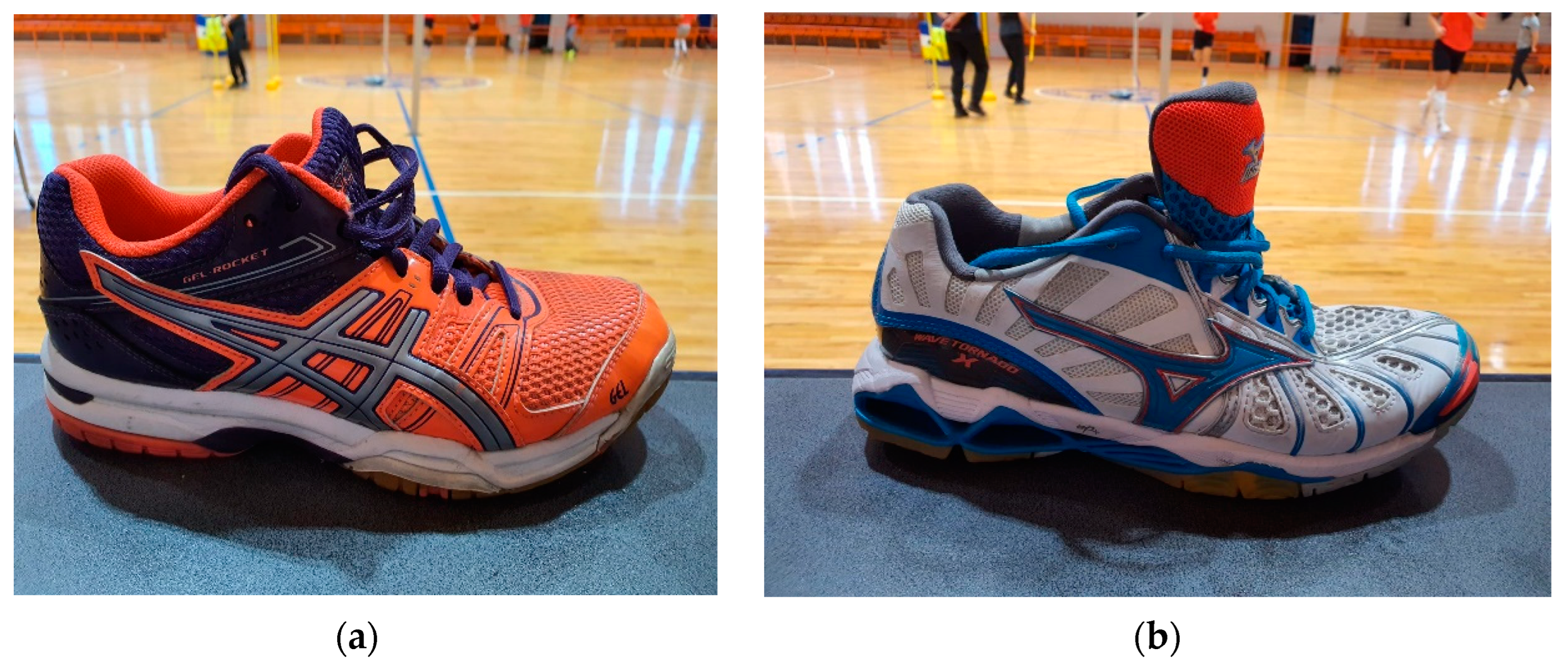
Thermography measurements were performed on five athletes (subjects) who wore Asics (subjects 1 and 2) and Mizuno (subjects 3, 4, and 5) sports shoes in a volleyball training session, as shown in Figure 3; footwear image and material characteristics for Asics and Mizuno shoes are shown in Figure 4. Polynomial regression is used to create a mathematical model and to predict temperature values outside the range of the experimental data.
The mechanical properties of the analyzed footwear were determined on the Nano Indenter Agilent G200, with the help of which Young’s modulus, Hardness at Maximum Load, Displacement at Maximum Load, Drift Correction, and Load at Max Load were determined according to ISO 14577 [42]. The external synthetic leather layer was analyzed (exposed to stress). Among the mechanical and thermal methods suffered, the Young’s modulus is modified. For future research, variation in Young’s modulus can be examined at other temperatures analyzed in the present article, both on synthetic leather and on synthetic fibers. The two pairs of footwear were exposed to the same temperature variations; one of the reasons why the heat transfer is different between the two models is due to mechanical properties of the two materials, which are differentiated by their different Young’s modulus values, shown in Table 1 for Asics and in Table 2 for Mizuno.
Based on the determined Young’s Modulus, it can be seen that the increase in the temperature in the range of 23.1 °C–32.7 °C on the shoe surface influences the increase in Young’s modulus linearly with the increase in the temperature in the range of 40 °C–100 °C [43]. In the research reviewed in the paper [43] on textile fibers, temperature has an influence on Young’s modulus; it can be observed that increasing temperature in the range of 40 °C–100 °C on textile fibers influences the increase in Young’s modulus. With increasing temperature, the structure of the material changes, influencing its mechanical properties.
In the research carried out in the present work on the textile material of the two types of footwear, it can be observed that the increase in temperature in the range 23.1 °C–32.7 °C influences the increase in Young’s modulus.
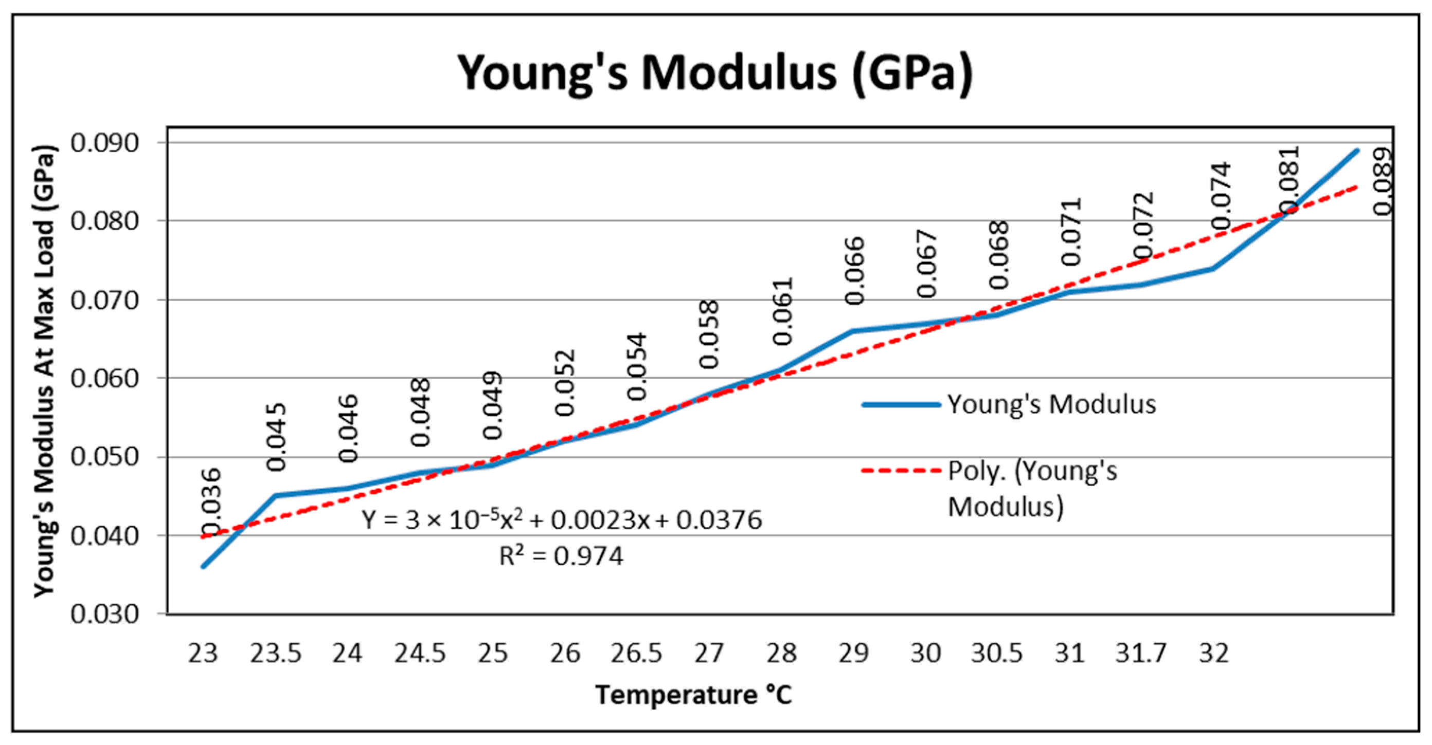
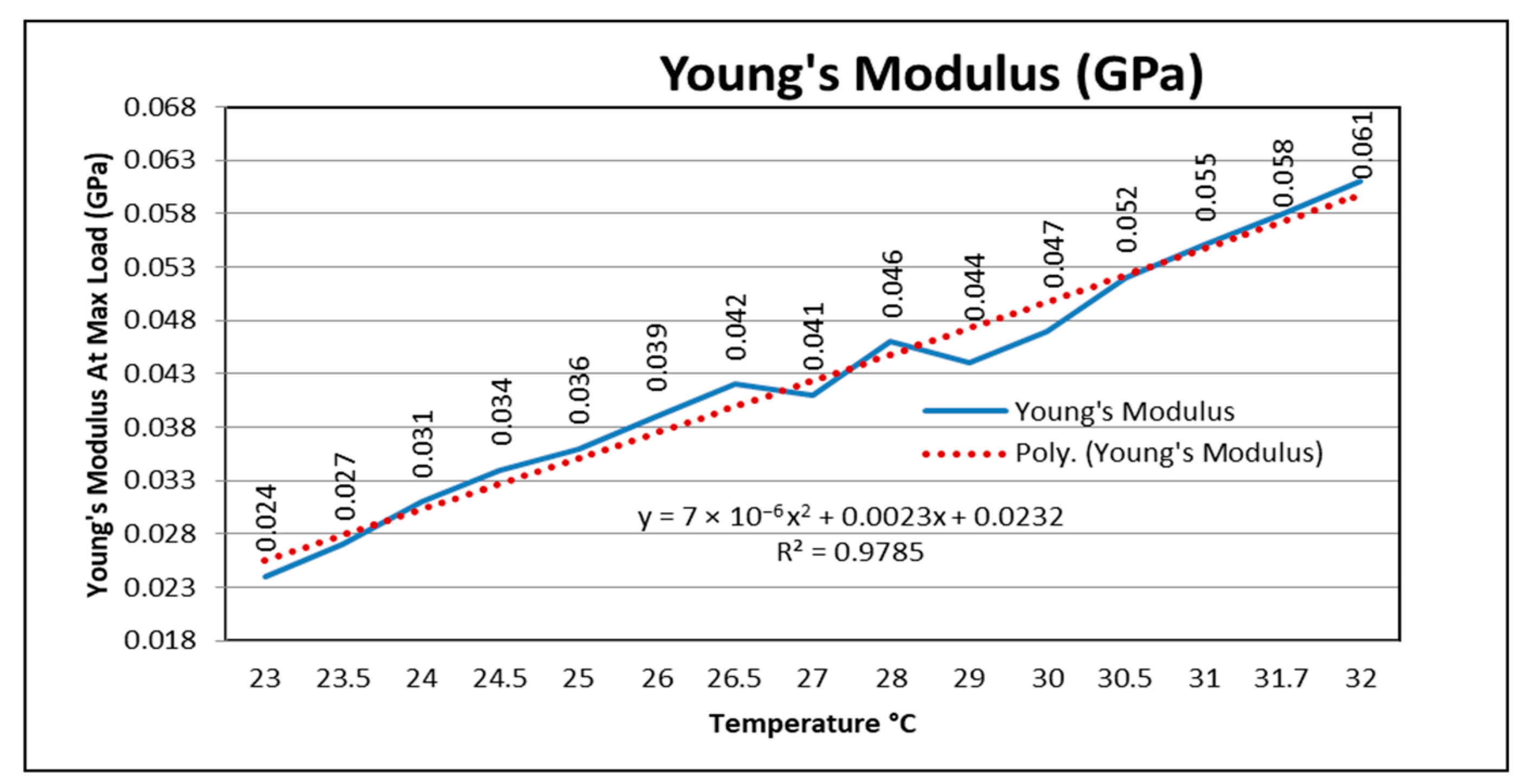
The Young’s modulus values shown in Table 1 and Table 2 are average values; Figure 5 and Figure 6 show the evolution of Young’s modulus for Asics footwear and Mizuno footwear as a function of temperature for the 23.1 °C–32.7 °C range.
The relationship obtained between temperature and Young’s modulus in the range 23.1 °C–32.7 °C as shown in Figure 5 for Asics footwear is a polynomial function of degree two (1).
y = 3 × 10⁻⁵x2 + 0.0023x + 0.0376
The coefficient of determining R2 established by the regression procedure is:
R2 = 0.974
The relationship obtained between temperature and Young’s modulus in the range 23.1 °C–32.7 °C as shown in Figure 6 for Mizuno footwear is a polynomial function of degree two (3).
y = 7 × 10−6x2 + 0.0023x + 0.0232
The coefficient of determining R2 established by the regression procedure is:
R2 = 0.9785

3. Results and Discussion

Thermographic recordings on sports shoes were made during training at five different times: moment zero (before starting the training), moment one at 2 min of training, moment two at 5 min of training, moment three at 15 min of training, and moment four at the end of the volleyball training. These recordings were made to identify the areas that ensure the best ventilation of the foot for comfort in movement.
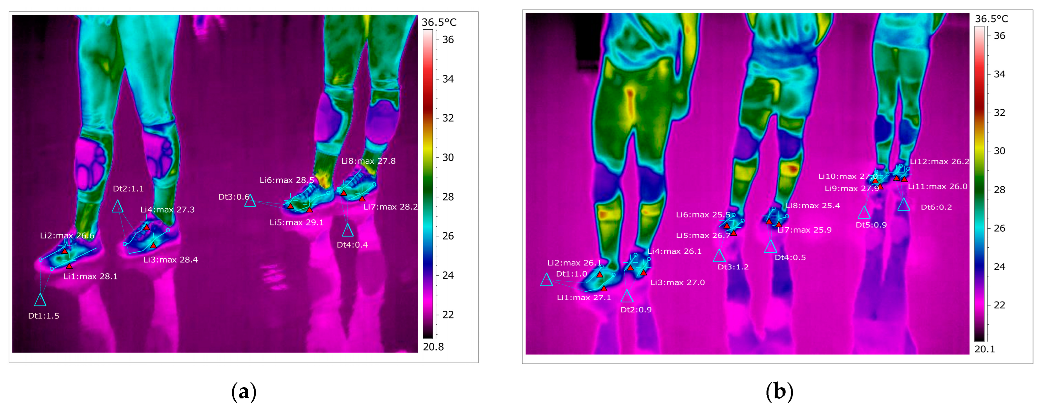
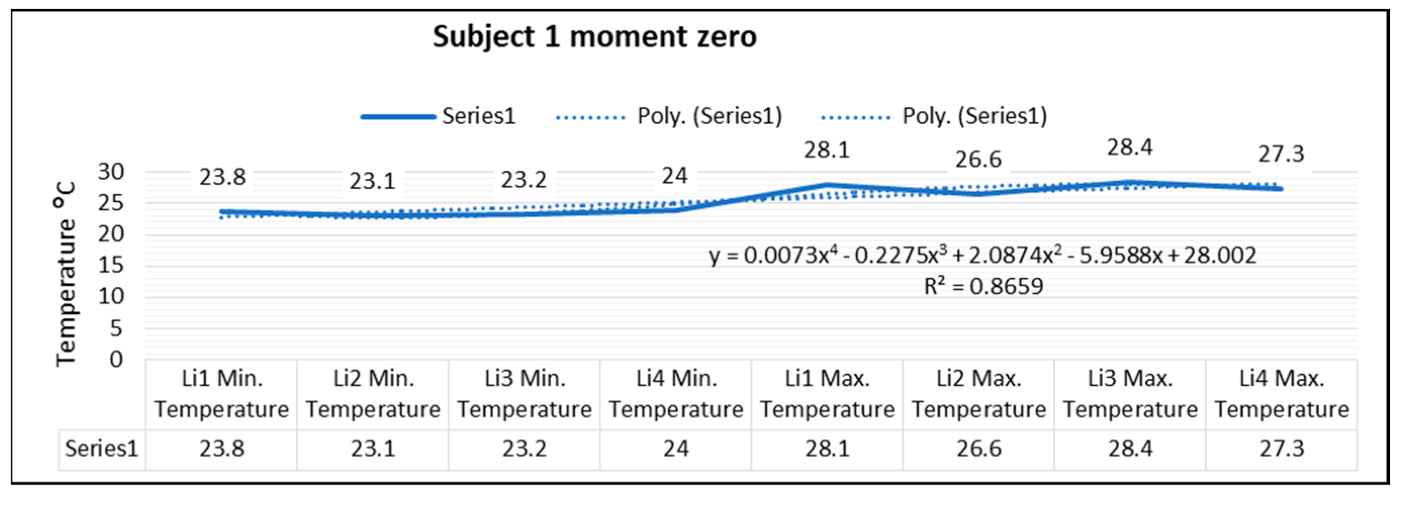
As shown in Figure 7 for the right foot of subject 1 at time zero (before the start of volleyball training), the maximum temperature along the line Li1, which is positioned on the central part of the foot, is 28.1 °C, and the minimum temperature is 23.8 °C.
The temperature variation along the Li1 line is 4.3 °C, and the emissivity is 0.83, at time zero for subject 1.
On the side along the Li2 line, the maximum temperature is 26.6 °C, and the minimum temperature is 23.1 °C, at time zero for subject 1. The temperature variation along the Li2 line is 3.5 °C, and the emissivity is 0.86 at time zero for subject 1.
For the left foot of subject 1 at time zero, the maximum temperature along the Li3 line positioned on the central side is 28.4 °C, and the minimum temperature is 23.2 °C.
The temperature variation along the Li3 line is 5.2 °C, and the emissivity is 0.81, at time zero for subject 1.
On the side along the Li4 line, the maximum temperature is 27.3 °C, and the minimum temperature is 24.0 °C, at time zero for subject 1.
The temperature variation along the line Li4 is 3.3 °C, and the emissivity is 0.83, at time zero for subject 1.
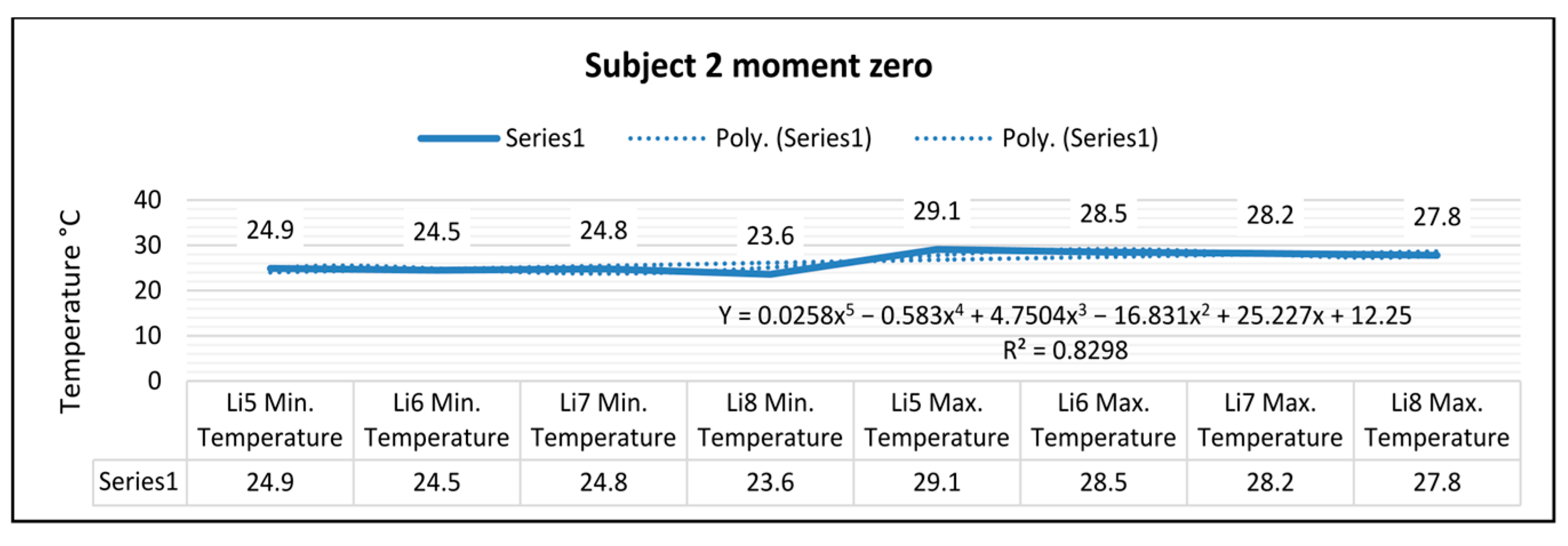
In Figure 7, for the right foot of subject 2 at time zero (before starting the volleyball training), the maximum temperature along the line Li5, which is positioned on the central part of the leg, is 29.1 °C, and the minimum temperature is 24.9 °C.
The temperature variation along the Li5 line is 4.2 °C, and the emissivity is 0.83, at time zero for subject 2.
On the side along the Li6 line, the maximum temperature is 28.5 °C, and the minimum temperature is 24.5 °C, at time zero for subject 2.
The temperature variation along the line Li6 is 4.0 °C, and the emissivity is 0.83, at time zero for subject 2.
For the left foot of subject 2 at time zero, the maximum temperature along the Li7 line positioned on the central side is 28.2 °C, and the minimum temperature is 24.8 °C.
The temperature variation along the Li7 line is 3.4 °C, and the emissivity is 0.83, at time zero for subject 2.
On the side along the Li8 line, the maximum temperature is 27.8 °C, and the minimum temperature is 23.6 °C, at time zero for subject 2.
The temperature variation along the line Li8 is 4.2 °C, and the emissivity is 0.83, at time zero for subject 2.
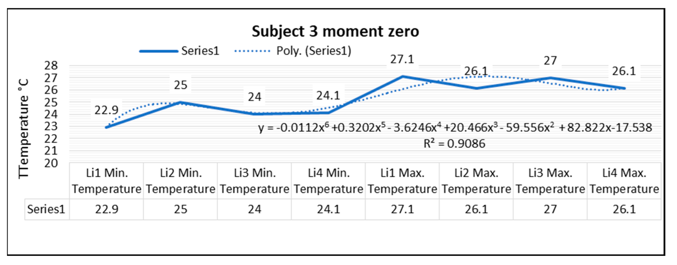
Thermography measurements for subject 3 for the right foot at time zero (before starting the volleyball training) show that the maximum temperature along the Li1 line, which is positioned on the center of the foot, is 27.1 °C, and the minimum temperature is 22.9 °C. The temperature variation along the Li1 line is 4.2 °C, and the emissivity is 0.83, at time zero for subject 3. On the side along the Li2 line, the maximum temperature is 26.1 °C, and the minimum temperature is 25.0 °C, at moment zero for subject 3. The temperature variation along the Li2 line is 1.1 °C, and the emissivity is 0.83, at moment zero for subject 3. For the left foot of subject 3 at time zero, the maximum temperature along the Li3 line positioned on the central side is 27.0 °C, and the minimum temperature is 24.0 °C. The temperature variation along the Li3 line is 3.0 °C, and the emissivity is 0.83, at time zero for subject 3. On the side along the Li4 line, the maximum temperature is 26.1 °C, and the minimum temperature is 24.1 °C, at time zero for subject 3.
The temperature variation along the line Li4 is 2.0 °C, and the emissivity is 0.83, at time zero for subject 3.
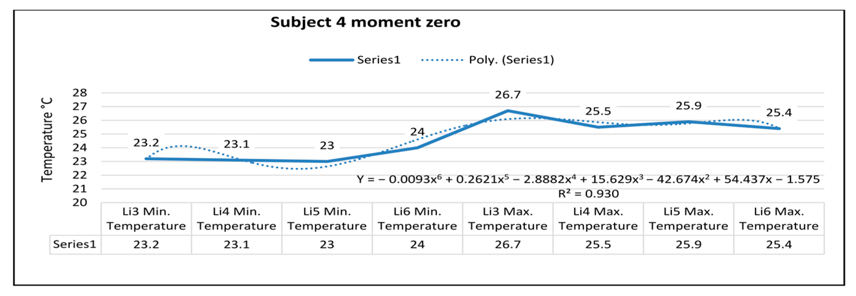
In Figure 7, for the right foot of subject 4 at time zero (before starting the volleyball training), the maximum temperature along the Li5 line, which is positioned on the center of the foot, is 26.7 °C, and the minimum temperature is 23.2 °C. The temperature variation along the Li5 line is 3.5 °C, and the emissivity is 0.83, at time zero for subject 4. On the side along the Li6 line, the maximum temperature is 25.5 °C, and the minimum temperature is 23.1 °C, at time zero for subject 4.
The temperature variation along the line is 2.4 °C, and the emissivity is 0.83, at time zero for subject 4.
For the left foot of subject 4 at time zero, the maximum temperature along the Li7 line positioned on the central side is 25.9 °C, and the minimum temperature is 23.0 °C.
The temperature variation along the Li7 line is 2.9 °C, and the emissivity is 0.83, at time zero for subject 4. On the side along the Li8 line, the maximum temperature is 25.4 °C, and the minimum temperature is 24.0 °C, at time zero for subject 4. The temperature variation along the line Li8 is 1.4 °C, and the emissivity is 0.83, at time zero for subject 4.
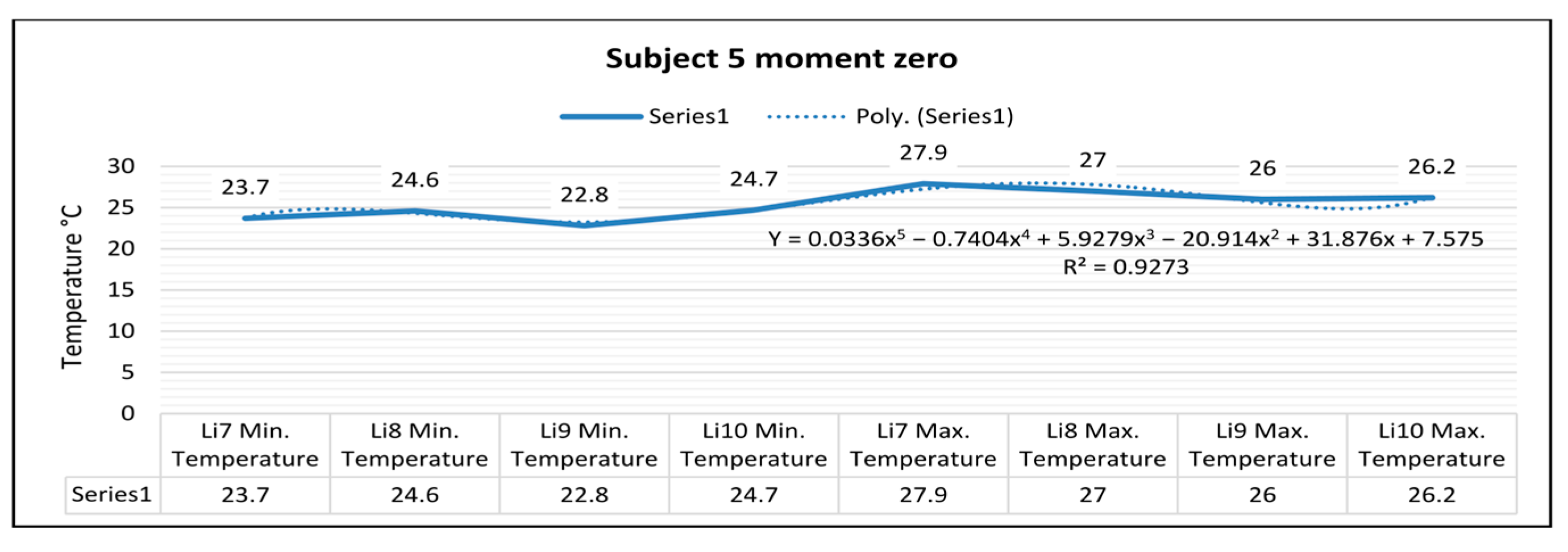
In Figure 7, for the right foot of subject 5 at time zero (before starting the volleyball training), the maximum temperature along the line Li9, which is positioned on the center of the foot, is 27.9 °C, and the minimum temperature is 23.7 °C. The temperature variation along the Li9 line is 4.2 °C, and the emissivity is 0.83, at time zero for subject 5. On the side along the Li10 line, the maximum temperature is 27.0 °C, and the minimum temperature is 24.6 °C, at time zero for subject 5. The temperature variation along the line Li10 is 2.4 °C, and the emissivity is 0.83, at time zero for subject 5. For the left foot of subject 5 at time zero, the maximum temperature along the Li11 line positioned on the central side is 26.0 °C, and the minimum temperature is 22.8 °C.
The temperature variation along the Li11 line is 3.2 °C, and the emissivity is 0.83, at time zero for subject 5. On the side along the Li12 line, the maximum temperature is 26.2 °C, and the minimum temperature is 24.7 °C, at zero time for subject 5. The temperature variation along the Li12 line is 1.4 °C, and the emissivity is 0.83, at zero time for subject 5. (Figure 8) shows the temperature variation along the subject lines on each footwear at time zero.
In the case of subject 1 at time zero, as shown in Figure 9, the relation obtained is a polynomial function of degree four (5).
Y = 0.0073x4 − 0.2275x3 + 2.0874x2 − 5.9588x + 28.002
The coefficient of determining R2 established by the regression procedure is:
R2 = 0.8659
In the case of subject 2 at time zero as shown in Figure 10, the relation obtained is a polynomial function of degree five (7).
Y = 0.0258x5 − 0.583x4 + 4.7504x3 − 16.831x2 + 25.227x + 12.25
The coefficient of determining R2 established by the regression procedure is:
R2 = 0.8298
In the case of subject 3 at time zero, as shown in Figure 11, the relation obtained is a polynomial function of degree six (9).
Y= −0.0112x6 + 0.3202x5 − 3.6246x4 + 20.466x3 − 59.556x2 + 82.822x − 17.538
The coefficient of determining R2 established by the regression procedure is:
R2 = 0.9086
In the case of subject 4 at time zero, as shown in Figure 12, the relation obtained is a polynomial function of degree six (11).
Y = −0.0093x6 + 0.2621x5 − 2.8882x4 + 15.629x3 − 42.674x2 + 54.437x − 1.575
The coefficient of determining R2 established by the regression procedure is:
R2 = 0.930
In the case of subject 5 at time zero, as shown in Figure 13, the relation obtained is a polynomial function of degree five (13).
Y = 0.0336x5 − 0.7404x4 + 5.9279x3 − 20.914x2 + 31.876x + 7.575
The coefficient of determining R2 established by the regression procedure is:
R2 = 0.9273
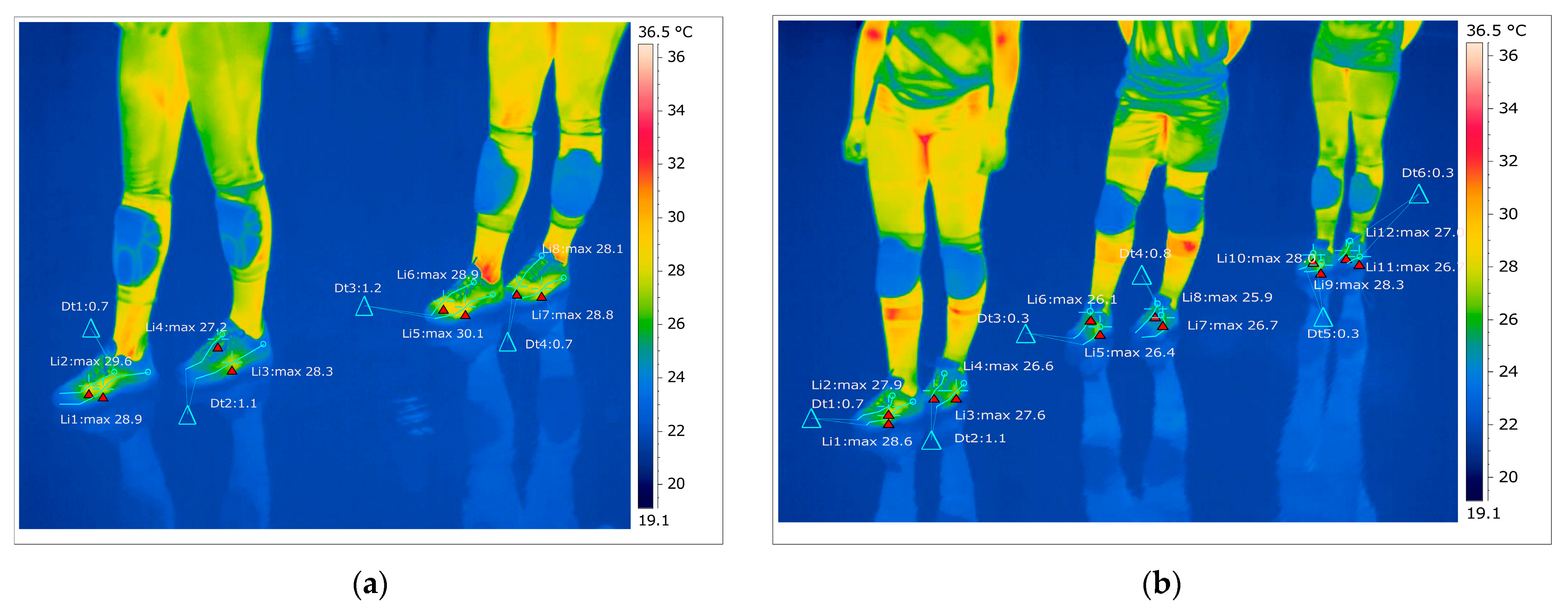
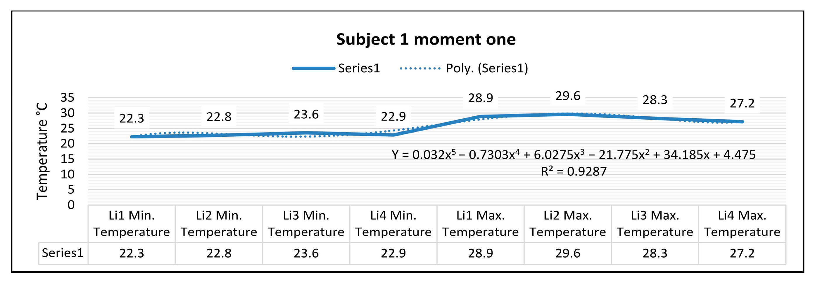
As shown in Figure 14, for the right foot of subject 1 at time one (two minutes of training), the maximum temperature along the line Li1, which is positioned on the center of the foot, is 28.9 °C, and the minimum temperature is 22.3 °C. The temperature variation along the Li1 line is 6.6 °C, and the emissivity is 0.83 at time one. On the side along the Li2 line, the maximum temperature is 29.6 °C, and the minimum temperature is 22.8 °C at time one. The temperature variation along the Li2 line is 6.9 °C, and the emissivity is 0.83 at time one.
For the left foot of subject 1 at time one, the maximum temperature along the Li3 line positioned on the central side is 28.3 °C, and the minimum temperature is 23.6 °C. The temperature variation along the Li3 line is 4.6 °C, and the emissivity is 0.83, for subject 1 at time one. On the side along the Li4 line, the maximum temperature is 27.2 °C, and the minimum temperature is 22.9 °C, for subject 1 at time one. The temperature variation along the Li4 line is 4.2 °C, and the emissivity is 0.83, for subject 1 at time one.
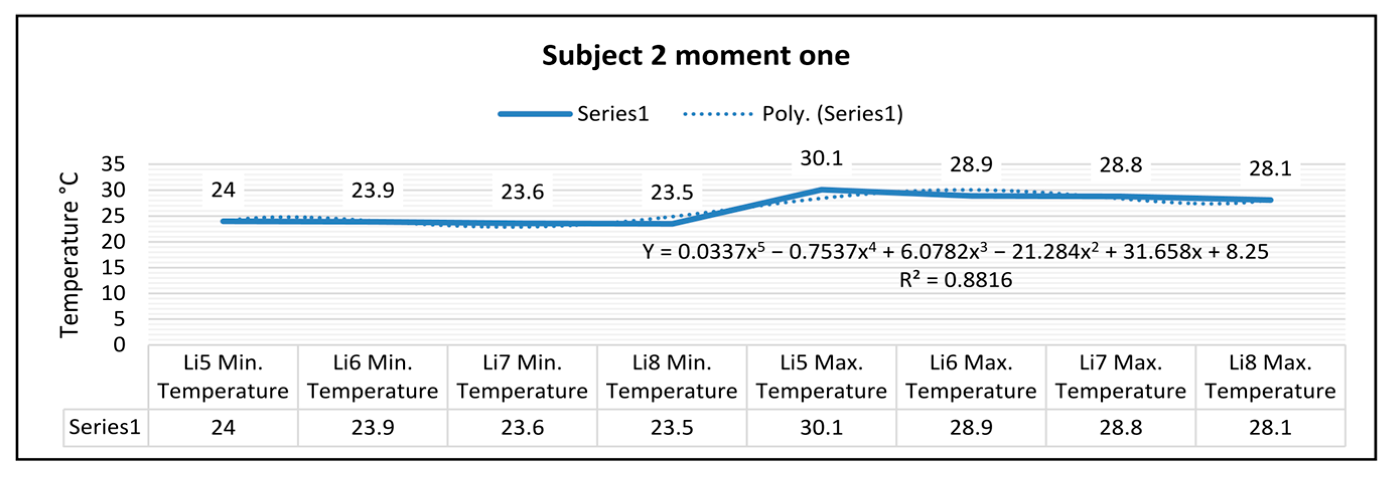
In Figure 14, for the right foot of subject 2 at time one (two minutes of training), the maximum temperature along the line Li5, which is positioned on the central part of the leg, is 30.1 °C, and the minimum temperature is 24.0 °C. The temperature variation along the Li5 line is 6.2 °C, and the emissivity is 0.83 at time one. On the side along the Li6 line, the maximum temperature is 28.9 °C, and the minimum temperature is 23.9 °C at time one. The temperature variation along the Li6 line is 4.9 °C, and the emissivity is 0.83 at time one.
For the left leg of subject 2 at time one, the maximum temperature along the Li7 line positioned on the central side is 28.8 °C, and the minimum temperature is 23.6 °C. The temperature variation along the Li7 line is 5.2 °C, and the emissivity is 0.83 at time one. On the side along the Li8 line, the maximum temperature is 28.1 °C, and the minimum temperature is 23.5 °C at time one. The temperature variation along the Li8 line is 4.6 °C, and the emissivity is 0.83 at time one.
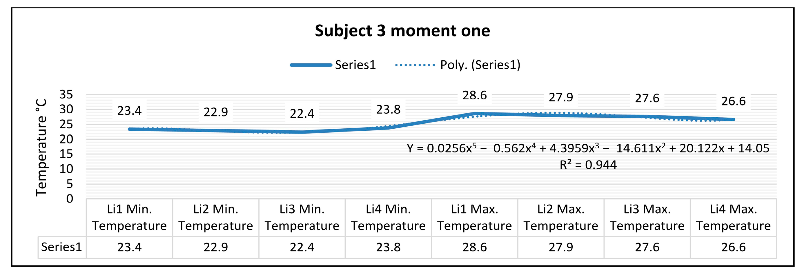
Thermography measurements afferent for subject 3 for the right foot at time one (two minutes of training) show that the maximum temperature along the Li1 line, which is positioned on the center of the foot, is 28.6 °C, and the minimum temperature is 23.4 °C. The temperature variation along the Li1 line is 5.2 °C, and the emissivity is 0.83 at time one. On the side along the Li2 line, the maximum temperature is 27.9 °C, and the minimum temperature is 22.9 °C, at time one. The temperature variation along the Li2 line is 4.9 °C, and the emissivity is 0.83 at time one.
For the left foot of subject 3 at time one, the maximum temperature along the Li3 line positioned on the central side is 27.6 °C, and the minimum temperature is 22.4 °C. The temperature variation along the Li3 line is 5.2 °C, and the emissivity is 0.83 at time one.
On the side along the Li4 line, the maximum temperature is 26.6 °C, and the minimum temperature is 23.8 °C, at time one. The temperature variation along the Li4 line is 2.8 °C, and the emissivity is 0.83 at time one.
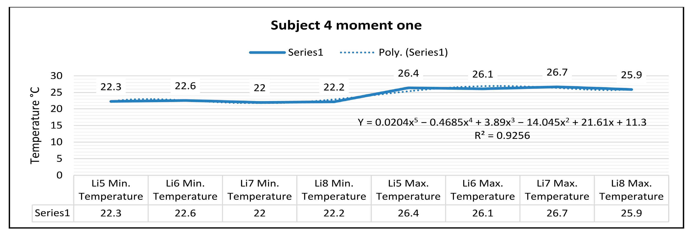
In Figure 14, for the right foot of subject 4 at time one (two minutes of training), the maximum temperature along the Li5 line, which is positioned on the center of the foot, is 26.4 °C, and the minimum temperature is 22.3 °C.
The temperature variation along the Li5 line is 4.1 °C, and the emissivity is 0.83 at time one.
On the side along the Li6 line, the maximum temperature is 26.1 °C, and the minimum temperature is 22.6 °C, at time one.
The temperature variation along the line is 3.6 °C, and the emissivity is 0.83, at time one.
For the left foot of subject 4 at time one, the maximum temperature along the Li7 line positioned on the central side is 26.7 °C, and the minimum temperature is 22.0 °C.
The temperature variation along the Li7 line is 4.6 °C, and the emissivity is 0.83 at time one. On the side along the Li8 line, the maximum temperature is 25.9 °C, and the minimum temperature is 22.2 °C at time one.
The temperature variation along the Li8 line is 3.7 °C, and the emissivity is 0.83 at time one.
In Figure 14, for the right foot of subject 5 at time one (two minutes of training), the maximum temperature along the line Li9, which is positioned on the central part of the foot, is 28.3 °C, and the minimum temperature is 23.0 °C.
The temperature variation along the Li9 line is 5.2 °C, and the emissivity is 0.83 at time one. On the side along the Li10 line, the maximum temperature is 28.0 °C, and the minimum temperature is 23.0 °C, at time one. The temperature variation along the Li10 line is 5.0 °C, and the emissivity is 0.83 at time one.
For the left foot of subject 5 at time one, the maximum temperature along the Li11 line positioned on the central side is 26.7 ° C, and the minimum temperature is 22.9 °C.
The temperature variation along the Li11 line is 3.8 °C, and the emissivity is 0.83 at time one. On the side along the Li12 line, the maximum temperature is 27.0 °C, and the minimum temperature is 23.3 °C, at moment one. The temperature variation along the Li12 line is 3.6 °C, and the emissivity is 0.83 at time one.
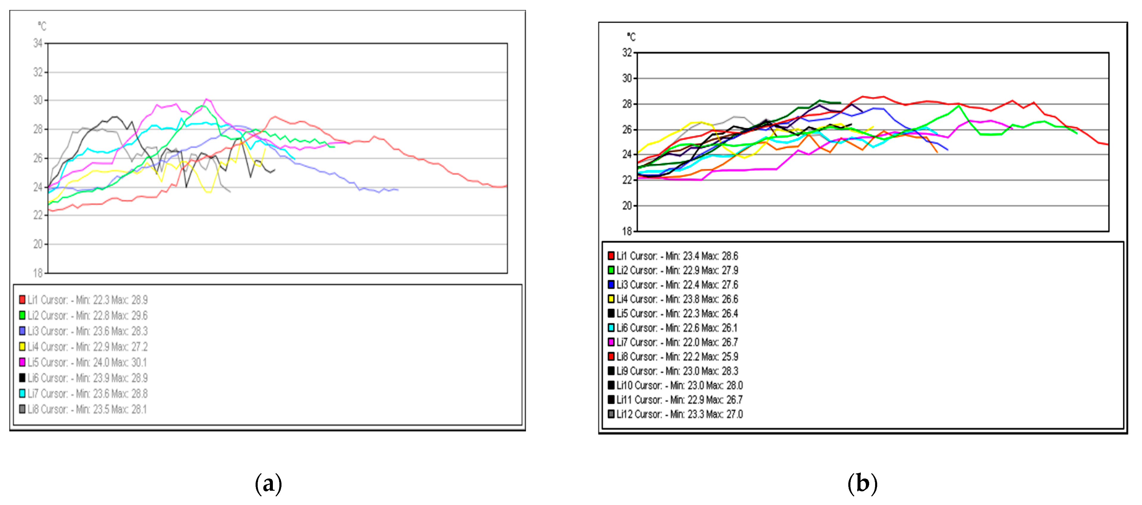
Figure 15 shows the temperature variation along the subject lines on each footwear at time one.
In the case of subject 1 at time one, as shown in Figure 16, the relation obtained is a polynomial function of degree five (15).
Y = 0.032x5 − 0.7303x4 + 6.0275x3 − 21.775x2 + 34.185x + 4.475
The coefficient of determining R2 established by the regression procedure is:
R2 = 0.9287
In the case of subject 2 at time one, as shown in Figure 17, the relation obtained is a polynomial function of degree five (17).
Y = 0.0337x5 − 0.7537x4 + 6.0782x3 − 21.284x2 + 31.658x + 8.25
The coefficient of determining R2 established by the regression procedure is:
R2 = 0.8816
In the case of subject 3 at time one, as shown in Figure 18, the relation obtained is a polynomial function of degree five (19).
Y = 0.0256x5 − 0.562x4 + 4.3959x3 − 14.611x2 + 20.122x + 14.05
The coefficient of determining R2 established by the regression procedure is:
R2 = 0.944
In the case of subject 4 at time one as shown in (Figure 19), the relation obtained is a polynomial function of degree five (21).
Y = 0.0204x5 − 0.4685x4 + 3.89x3 − 14.045x2 + 21.61x + 11.3
The coefficient of determining R2 established by the regression procedure is:
R2 = 0.9256
In the case of subject 5 at time one, as shown in Figure 20, the relation obtained is a polynomial function of degree five (23).
Y = 0.0335x5 − 0.7396x4 + 5.8882x3 − 20.439x2 + 30.4x + 7.825
The coefficient of determining R2 established by the regression procedure is:
R2 = 0.9431
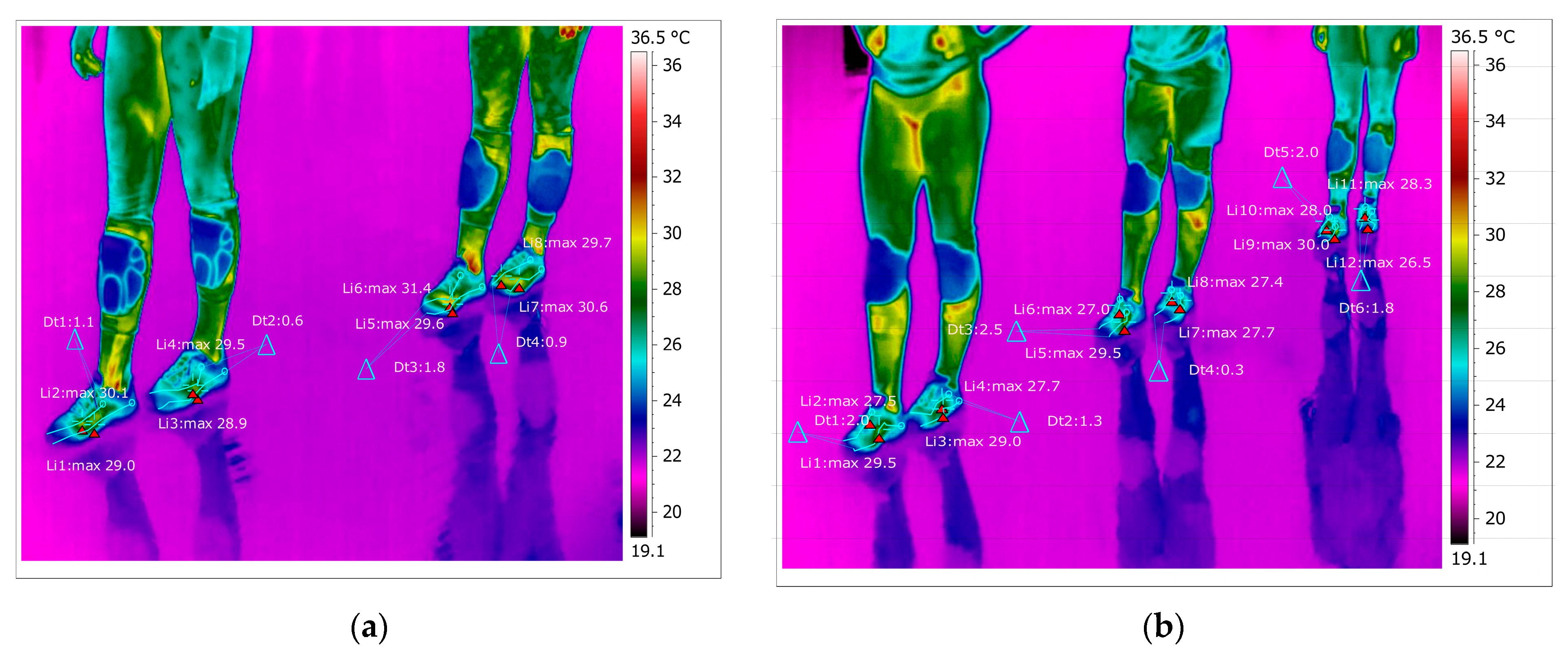
As shown in Figure 21, for the right foot of subject 1 at time two (five minutes of training), the maximum temperature along the line Li1, which is positioned on the center of the foot, is 29.0 °C, and the minimum temperature is 22.1 °C. The temperature variation along the Li1 line is 6.9 °C, and the emissivity is 0.83 at time two. On the side along the Li2 line, the maximum temperature is 30.1 °C, and the minimum temperature is 22.5 °C at time two. The temperature variation along the Li2 line is 7.6 °C, and the emissivity is 0.83 at time two. For the left foot of subject 1 at time two, the maximum temperature along the Li3 line positioned on the central side is 28.9 °C, and the minimum temperature is 23.5 °C.
The temperature variation along the Li3 line is 5.5 °C, and the emissivity is 0.83, for subject 1 at time two. On the side along the Li4 line, the maximum temperature is 29.5 °C, and the minimum temperature is 23.0 °C, for subject 1 at time two. The temperature variation along the Li4 line is 6.5 °C, and the emissivity is 0.83, for subject 1 at time two.
In Figure 21, for the right foot of subject 2 at time two (five minutes of training), the maximum temperature along the Li5 line, which is positioned on the center of the foot, is 29.6 °C, and the minimum temperature is 23.3 °C. The temperature variation along the Li5 line is 6.2 °C, and the emissivity is 0.83 at time two. On the side along the Li6 line, the maximum temperature is 31.4 °C, and the minimum temperature is 25.8 °C at time two.
The temperature variation along the Li6 line is 5.6 °C, and the emissivity is 0.83 at time two. For the left foot of subject 2 at time two, the maximum temperature along the Li7 line positioned on the central side is 30.6 °C, and the minimum temperature is 25.5 °C.
The temperature variation along the Li7 line is 5.1 °C, and the emissivity is 0.83 at time two. On the side along the Li8 line, the maximum temperature is 29.7 °C, and the minimum temperature is 24.9 °C, at time two. The temperature variation along the Li8 line is 4.8 °C, and the emissivity is 0.83 at the second moment. Thermography measurements afferent for subject 3 for the right foot at time two (five minutes of training) show that the maximum temperature along the Li1 line, which is positioned on the central part of the foot, is 29.5 °C, and the minimum temperature is 23.0 °C. The temperature variation along the Li1 line is 6.6 °C, and the emissivity is 0.83 at time two. On the side along the Li2 line, the maximum temperature is 27.5 °C, and the minimum temperature is 22.5 °C at time two. The temperature variation along the Li2 line is 5.0 °C, and the emissivity is 0.83 at time two. For the left leg of subject 3 at time two, the maximum temperature along the Li3 line positioned on the central side is 29.0 °C, and the minimum temperature is 23.5 °C. The temperature variation along the Li3 line is 5.5 °C, and the emissivity is 0.83 at time two. On the side along the Li4 line, the maximum temperature is 27.7 °C, and the minimum temperature is 25.2 °C, at time two. The temperature variation along the Li4 line is 2.5 °C, and the emissivity is 0.83 at the second moment.
In Figure 21, for the right foot of subject 4 at time two (five minutes of training), the maximum temperature along the Li5 line, which is positioned on the central part of the foot, is 29.5 °C, and the minimum temperature is 23.6 °C. The temperature variation along the Li5 line is 5.9 °C, and the emissivity is 0.83 at time two. On the side along the Li6 line, the maximum temperature is 27.0 °C, and the minimum temperature is 23.2 °C, at time two. The temperature variation along the line is 3.7 °C, and the emissivity is 0.83 at time two. For the left foot of subject 4 at time two, the maximum temperature along the Li7 line positioned on the central side of the foot is 27.7 °C, and the minimum temperature is 22.6 °C. The temperature variation along the Li7 line is 5.1 °C, and the emissivity is 0.83 at time two. On the side along the Li8 line, the maximum temperature is 27.4 °C, and the minimum temperature is 22.5 °C, at time two. The temperature variation along the Li8 line is 4.9 °C, and the emissivity is 0.83 at time two.
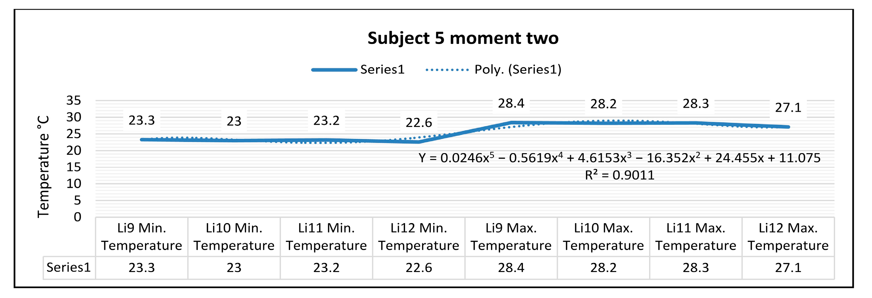
In Figure 21, for the right foot of subject 5 at time two (five minutes of training), the maximum temperature along the line Li9, which is positioned on the central part of the foot, is 30.0 °C, and the minimum temperature is 23.3 °C. The temperature variation along the Li9 line is 6.8 °C, and the emissivity is 0.83 at time two. On the side along the Li10 line, the maximum temperature is 28.0 °C, and the minimum temperature is 23.0 °C, at time two. The temperature variation along the Li10 line is 5.0 °C, and the emissivity is 0.83 at time two. For the left foot of subject 5 at time two, the maximum temperature along the Li11 line positioned on the central side of the foot is 28.3 °C, and the minimum temperature is 23.2 °C. The temperature variation along the Li11 line is 5.1 °C, and the emissivity is 0.83 at time two. On the side along the Li12 line, the maximum temperature is 26.5 °C, and the minimum temperature is 22.6 °C at time two. The temperature variation along the Li12 line is 3.9 °C, and the emissivity is 0.83 at time two.
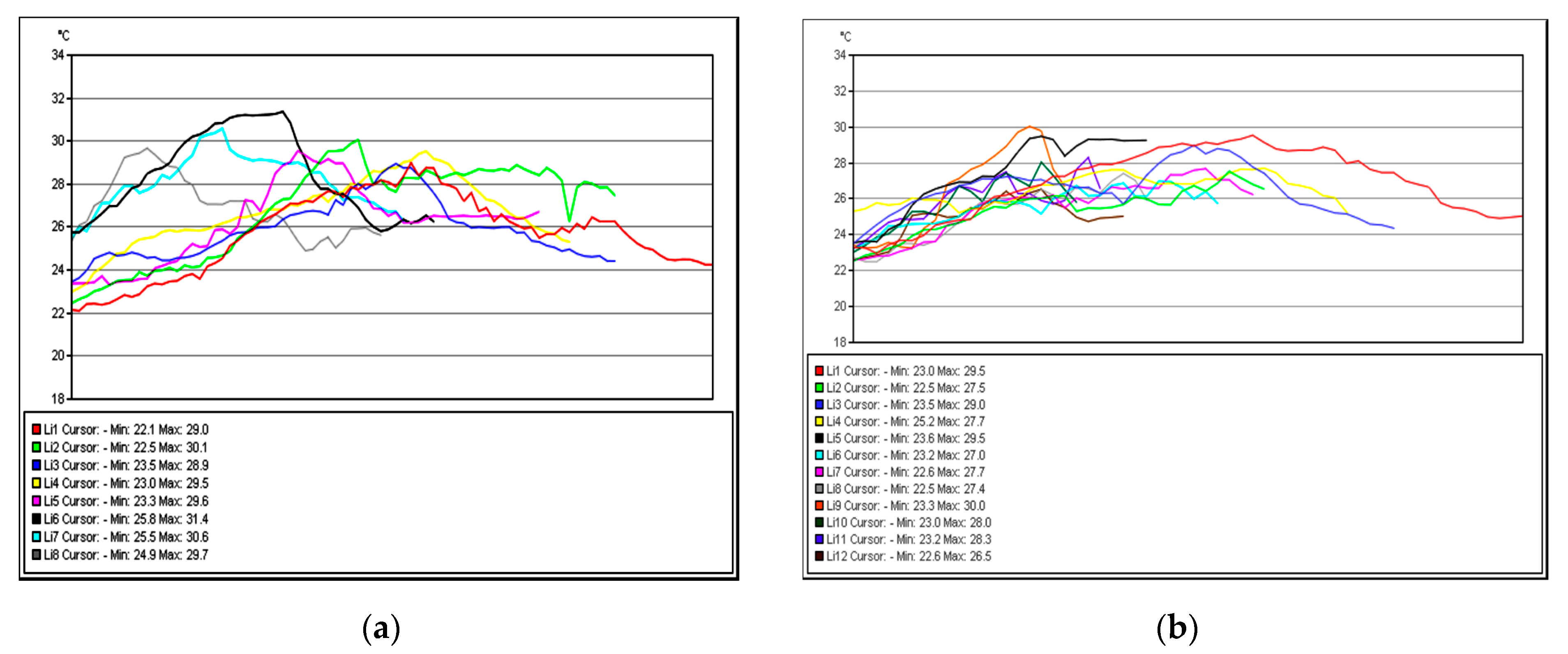
Figure 22 shows the temperature variation along the subject lines on each footwear at time two.
The graphs in Figure 23 show the temperature variation along the subject lines on each shoe at time two.
In the case of subject 1 at time two, as shown in Figure 23, the relation obtained is a polynomial function of degree five (25).
Y = 0.0342x5 − 0.77x4 + 6.2742x3 − 22.391x2 + 34.781x + 4.075
The coefficient of determining R2 established by the regression procedure is:
R2 = 0.949
In the case of subject 2 at time two, as shown in Figure 24, the relation obtained is a polynomial function of degree five (23).
Y = 0.0337x5 − 0.7988x4 + 6.9294x3 − 26.798x2 + 45.724x − 1.85
The coefficient of determining R2 established by the regression procedure is:
R2 = 0.973
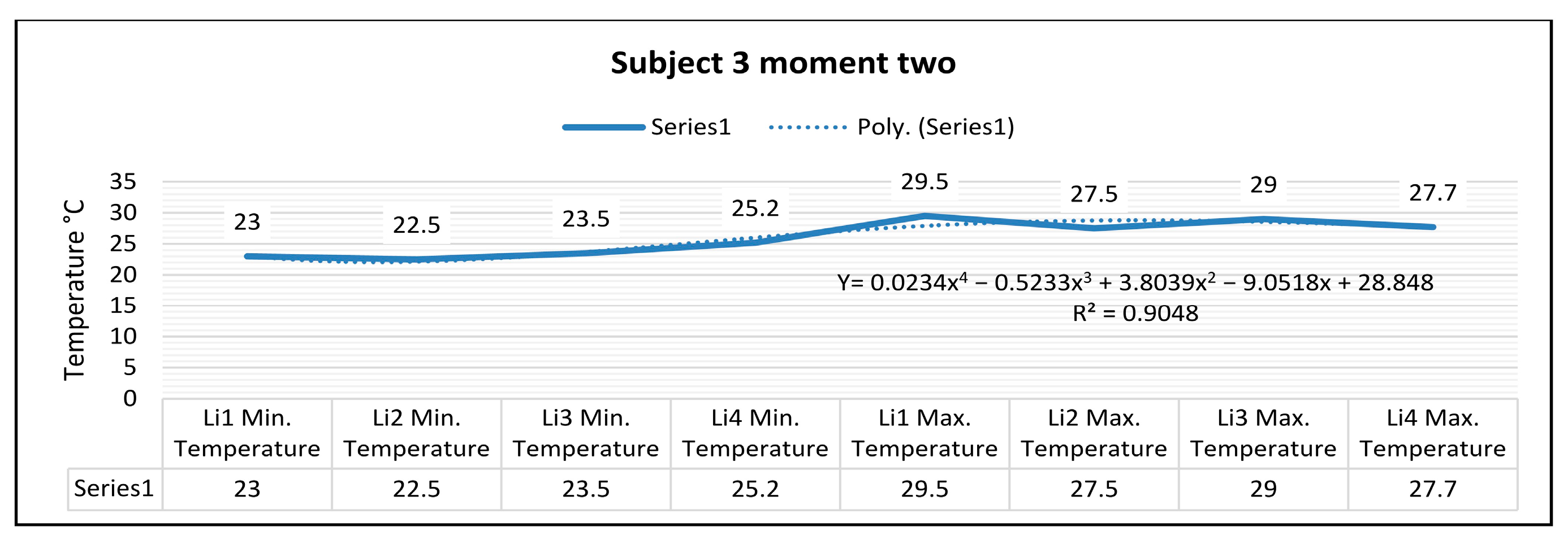
In the case of subject 3 at time two, as shown in Figure 25, the relation obtained is a polynomial function of degree four (29).
Y = 0.0234x4 − 0.5233x3 + 3.8039x2 − 9.0518x + 28.848
The coefficient of determining R2 established by the regression procedure is:
R2 = 0.9048
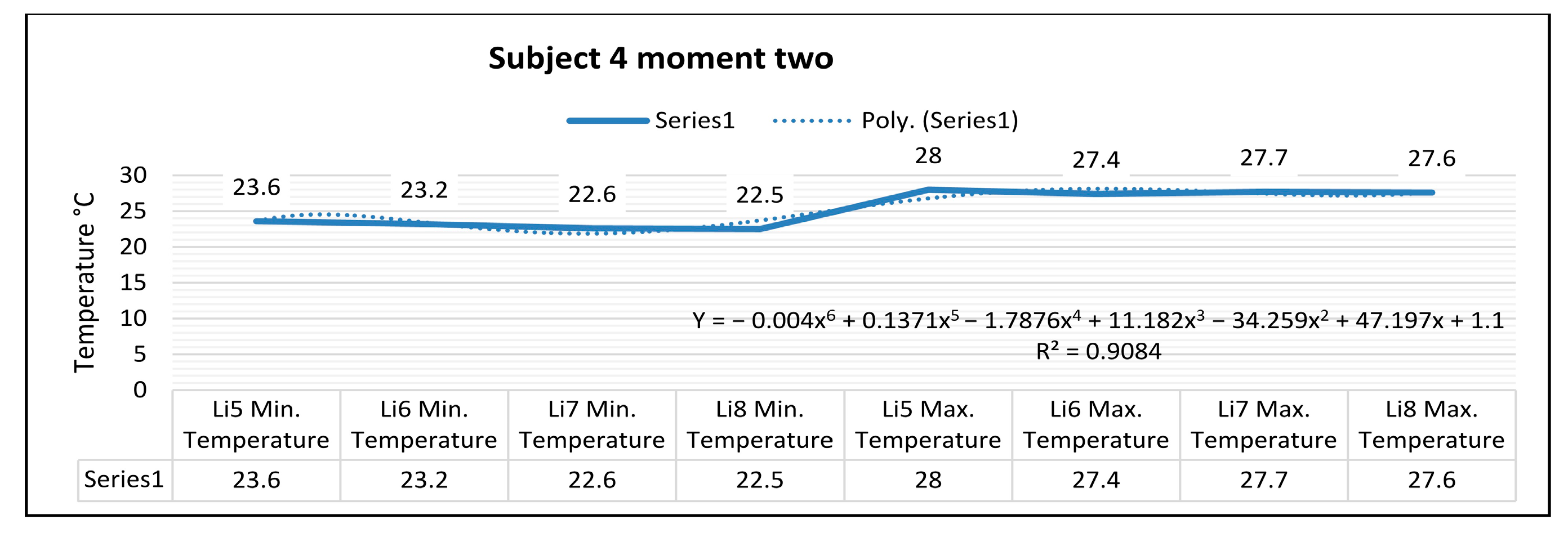
In the case of subject 4 at time two, as shown in Figure 26, the relation obtained is a polynomial function of degree six (31).
Y = −0.004x6 + 0.1371x5 − 1.7876x4 + 11.182x3 − 34.259x2 + 47.197x + 1.1
The coefficient of determining R2 established by the regression procedure is:
R2 = 0.9084
In the case of subject 5 at time two, as shown in Figure 27, the relation obtained is a polynomial function of degree five (33).
Y = 0.0246x5 − 0.5619x4 + 4.6153x3 − 16.352x2 + 24.455x + 11.075
The coefficient of determining R2 established by the regression procedure is:
R2 = 0.9011
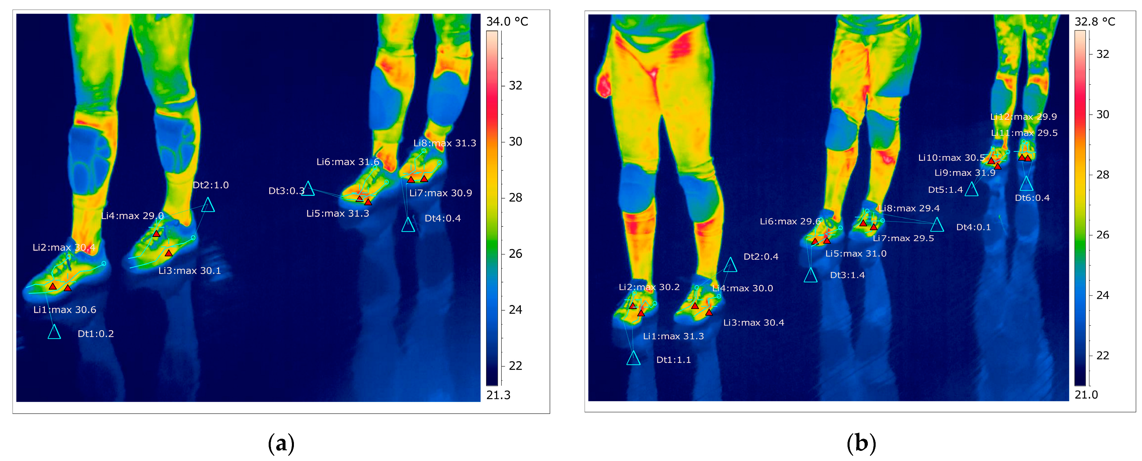
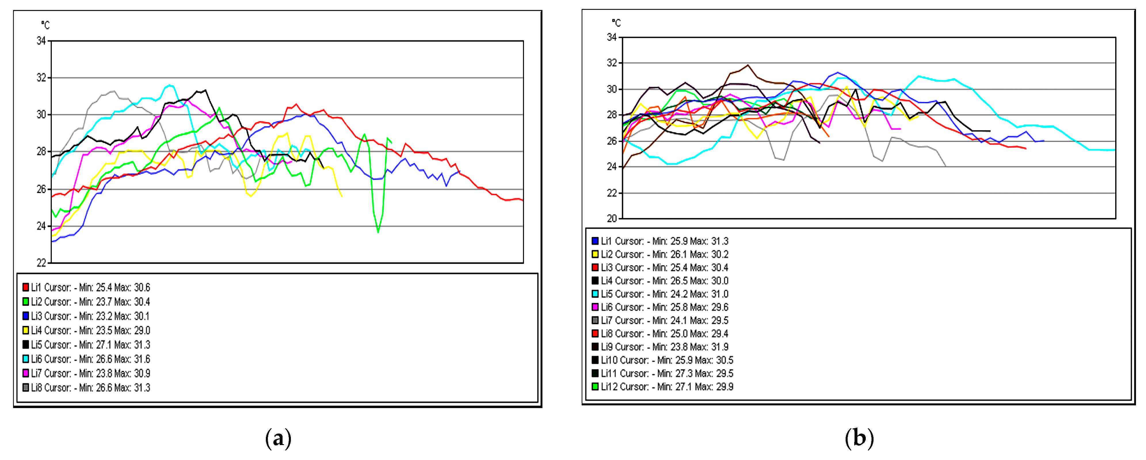
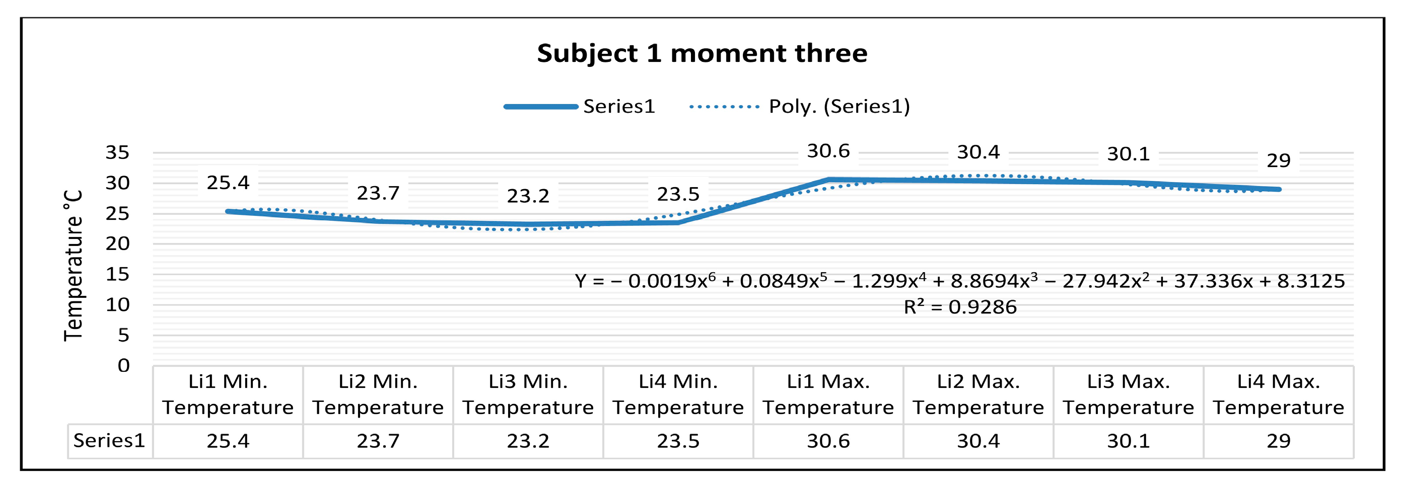
As shown in Figure 28, for the right foot of subject 1 at time three (15 min of training), the maximum temperature along the line Li1, which is positioned on the center of the foot, is 30.6 °C, and the minimum temperature is 25.4 °C.
The temperature variation along the Li1 line is 5.2 °C, and the emissivity is 0.83 at time three. On the side along the Li2 line, the maximum temperature is 30.4 °C, and the minimum temperature is 23.7 °C, at time three. The temperature variation along the Li2 line is 6.7 °C, and the emissivity is 0.83 at time three. For the left foot of subject 1 at time three, the maximum temperature along the Li3 line positioned on the central side is 30.1 °C, and the minimum temperature is 23.2 °C. The temperature variation along the Li3 line is 6.9 °C, and the emissivity is 0.83, for subject 1 at time three. On the side along the Li4 line, the maximum temperature is 29.0 °C, and the minimum temperature is 23.5 °C, for subject 1 at time three. The temperature variation along the Li4 line is 5.6 °C, and the emissivity is 0.83, for subject 1 at time three.
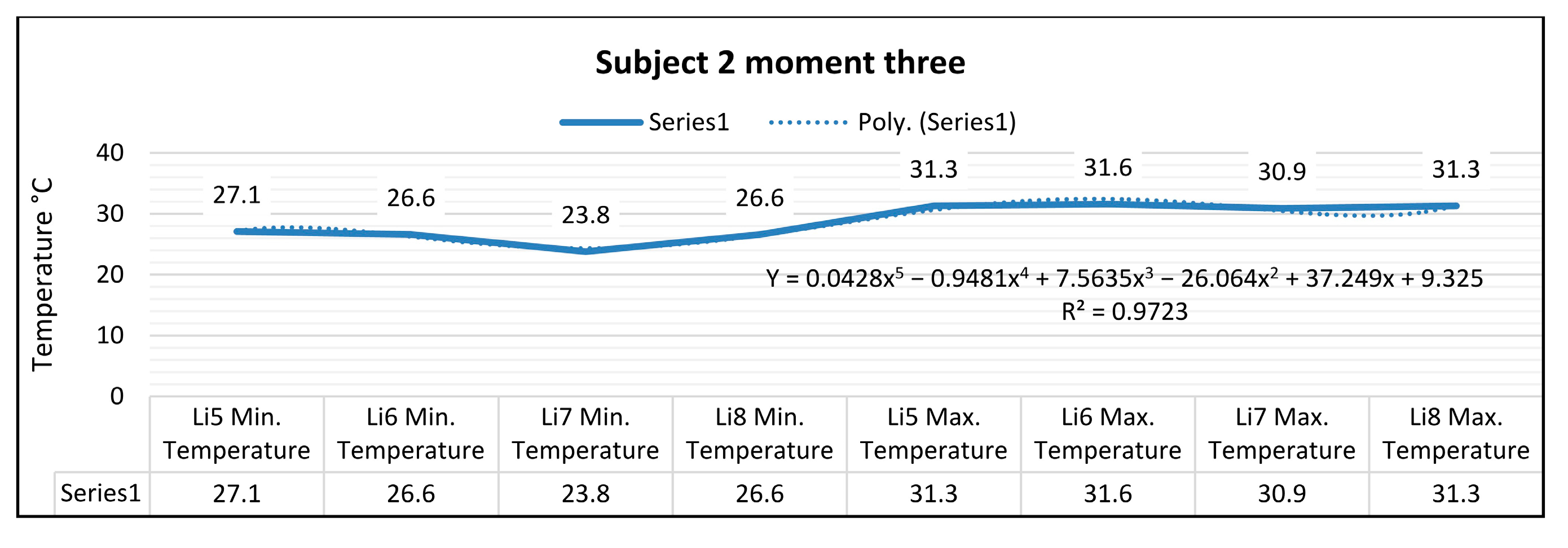
In Figure 28, for the right foot of subject 2 at time three (15 min of training), the maximum temperature along the Li5 line, which is positioned on the center of the leg, is 31.3 °C, and the minimum temperature is 27.1 °C. The temperature variation along the Li5 line is 4.2 °C, and the emissivity is 0.83 at time three. On the side along the Li6 line, the maximum temperature is 31.6 °C, and the minimum temperature is 26.6 °C at time three.
The temperature variation along the Li6 line is 5.0 °C, and the emissivity is 0.83 at time three. For the left foot of subject 2 at time three, the maximum temperature along the Li7 line positioned on the central side is 30.9 °C, and the minimum temperature is 23.8 °C. The temperature variation along the Li7 line is 7.1 °C, and the emissivity is 0.83 at time three.
On the side along the Li8 line, the maximum temperature is 31.3 °C, and the minimum temperature is 26.6 °C at time three. The temperature variation along the Li8 line is 4.7 °C, and the emissivity is 0.83 at time three.
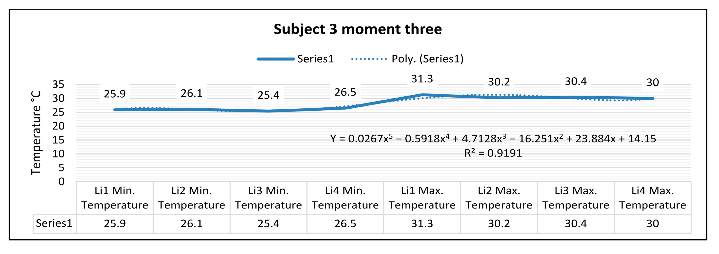
Thermography measurements for subject 3 for the right foot at time three (15 min of training) show that the maximum temperature along the Li1 line, which is positioned on the center of the foot, is 31.3 °C, and the minimum temperature is 25.9 °C.
The temperature variation along the Li1 line is 5.4 °C, and the emissivity is 0.83 at time three.
On the side along the Li2 line, the maximum temperature is 30.2 °C, and the minimum temperature is 26.1 °C at time three. The temperature variation along the Li2 line is 4.1 °C, and the emissivity is 0.83 at time three.
For the left foot of subject 3 at time three, the maximum temperature along the Li3 line positioned on the central side is 30.4 °C, and the minimum temperature is 25.4 °C. The temperature variation along the Li3 line is 5.0 °C, and the emissivity is 0.83 at time three.
On the side along the Li4 line, the maximum temperature is 30.2 °C, and the minimum temperature is 26.5 °C at time three. The temperature variation along the Li4 line is 3.5 °C, and the emissivity is 0.83 at time three.
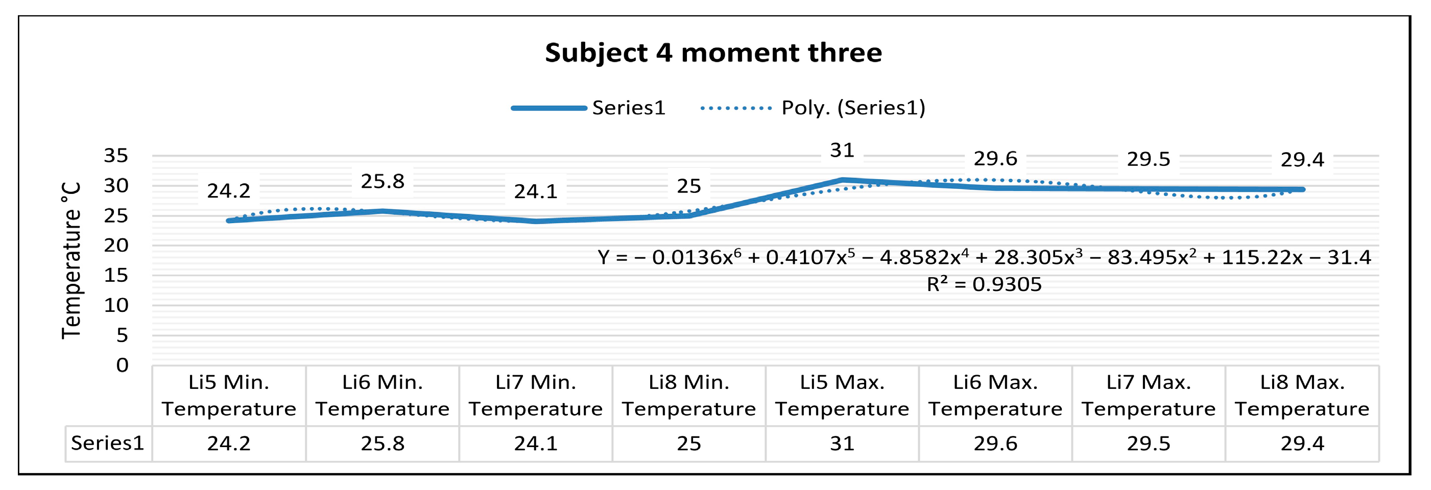
In Figure 28, for the right foot of subject 4 at time three (15 min of training), the maximum temperature along the Li5 line, which is positioned on the central part of the leg, is 31.0 °C, and the minimum temperature is 24.2 °C.
The temperature variation along the Li5 line is 6.8 °C, and the emissivity is 0.83 at time three. On the side along the Li6 line, the maximum temperature is 29.6 °C, and the minimum temperature is 25.8 °C, at time three. The temperature variation along the line is 3.8 °C, and the emissivity is 0.83, at time three.
For the left foot of subject 4 at time three, the maximum temperature along the Li7 line positioned on the central side is 29.5 °C, and the minimum temperature is 24.1 °C. The temperature variation along the Li7 line is 5.4 °C, and the emissivity is 0.83 at time three.
On the side along the Li8 line, the maximum temperature is 29.4 °C, and the minimum temperature is 25.0 °C, at time three. The temperature variation along the Li8 line is 4.5 °C, and the emissivity is 0.83 at time three.
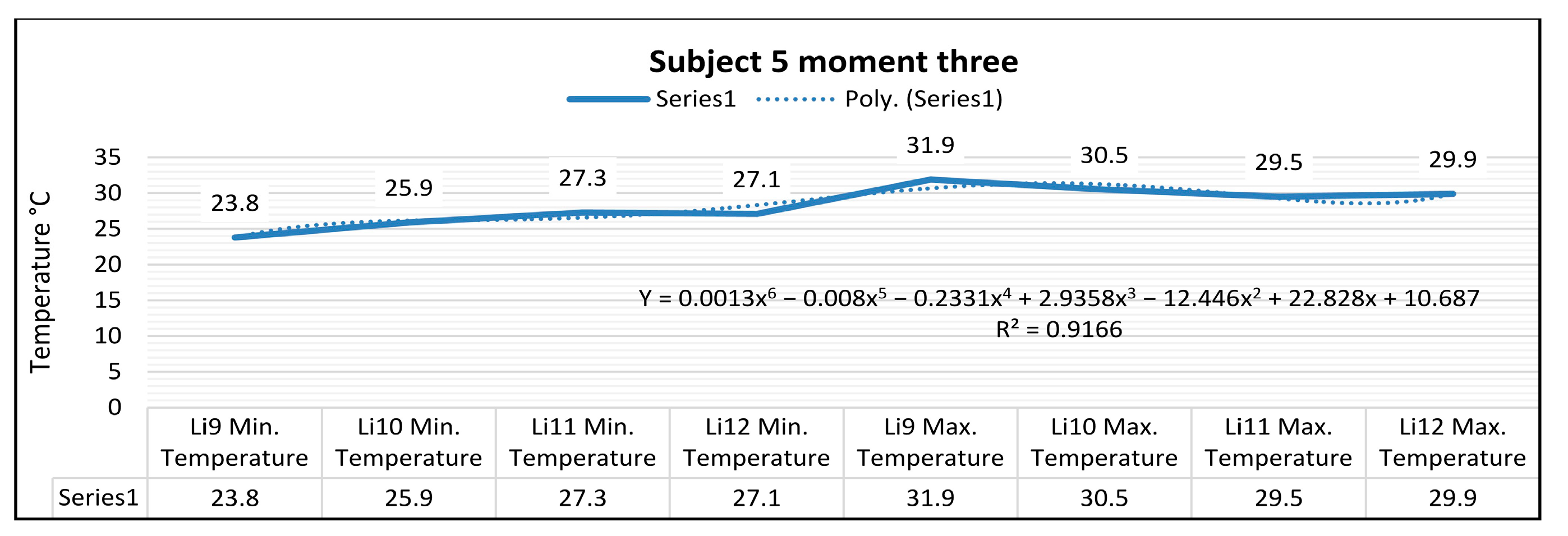
In Figure 28, for the right foot of subject 5 at time three (15 min of training), the maximum temperature along the Li9 line, which is positioned on the center of the leg, is 31.9 °C, and the minimum temperature is 23.8 °C.
The temperature variation along the Li9 line is 8.0 °C, and the emissivity is 0.83 at time three. On the side along the Li10 line, the maximum temperature is 30.5 °C, and the minimum temperature is 25.9 °C at time three. The temperature variation along the Li10 line is 4.6 °C, and the emissivity is 0.83 at time three.
For the left foot of subject 5 at time three, the maximum temperature along the Li11 line positioned on the central side is 29.5 °C, and the minimum temperature is 27.3 °C. The temperature variation along the Li11 line is 2.2 °C, and the emissivity is 0.83 at time three.
On the side along the Li12 line, the maximum temperature is 29.9 °C, and the minimum temperature is 27.1 °C, at time three. The temperature variation along the Li12 line is 2.7 °C, and the emissivity is 0.83 at time three.
Figure 29 shows the temperature variation along the subject lines on each shoe at time three.
In the case of subject 1 at time three, as shown in Figure 30, the relation obtained is a polynomial function of degree six (35).
Y = −0.0019x6 + 0.0849x5 − 1.299x4 + 8.8694x3 − 27.942x2 + 37.336x + 8.3125
The coefficient of determining R2 established by the regression procedure is:
R2 = 0.9286
In the case of subject 2 at time three, as shown in Figure 31, the relation obtained is a polynomial function of degree five (37).
Y = 0.0428x5 − 0.9481x4 + 7.5635x3 − 26.064x2 + 37.249x + 9.325
The coefficient of determining R2 established by the regression procedure is:
R2 = 0.9723
In the case of subject 3 at time three as shown in Figure 32, the relation obtained is a polynomial function of degree five (39).
Y = 0.0267x5 − 0.5918x4 + 4.7128x3 − 16.251x2 + 23.884x + 14.15
The coefficient of determining R2 established by the regression procedure is:
R2 = 0.9191
In the case of subject 4 at time three, as shown in Figure 33, the relation obtained is a polynomial function of degree six (41).
Y = −0.0136x6 + 0.4107x5 − 4.8582x4 + 28.305x3 − 83.495x2 + 115.22x − 31.4
The coefficient of determining R2 established by the regression procedure is:
R2 = 0.9305
In the case of subject 5 at time three, as shown in Figure 34, the relation obtained is a polynomial function of degree six (43).
Y = 0.0013x6 − 0.008x5 − 0.2331x4 + 2.9358x3 − 12.446x2 + 22.828x + 10.687
The coefficient of determining R2 established by the regression procedure is:
R2 = 0.9166
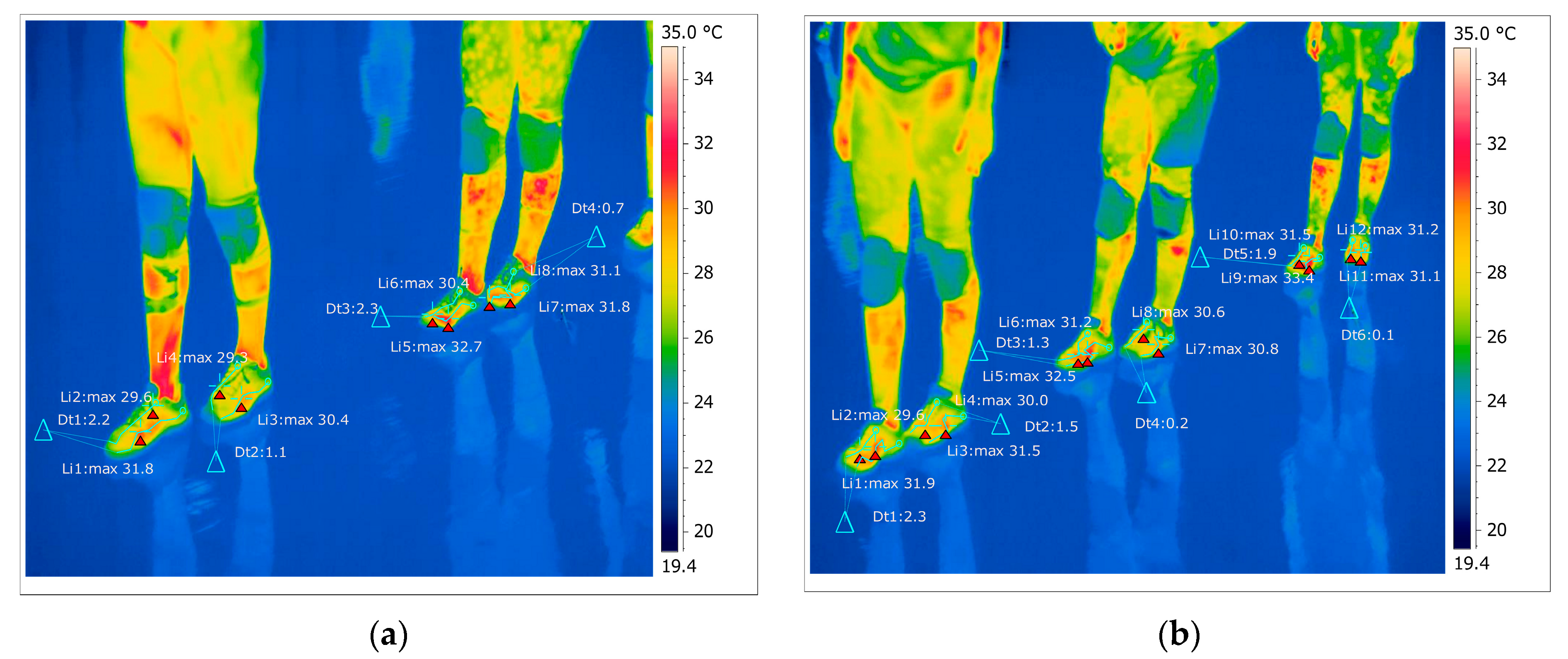
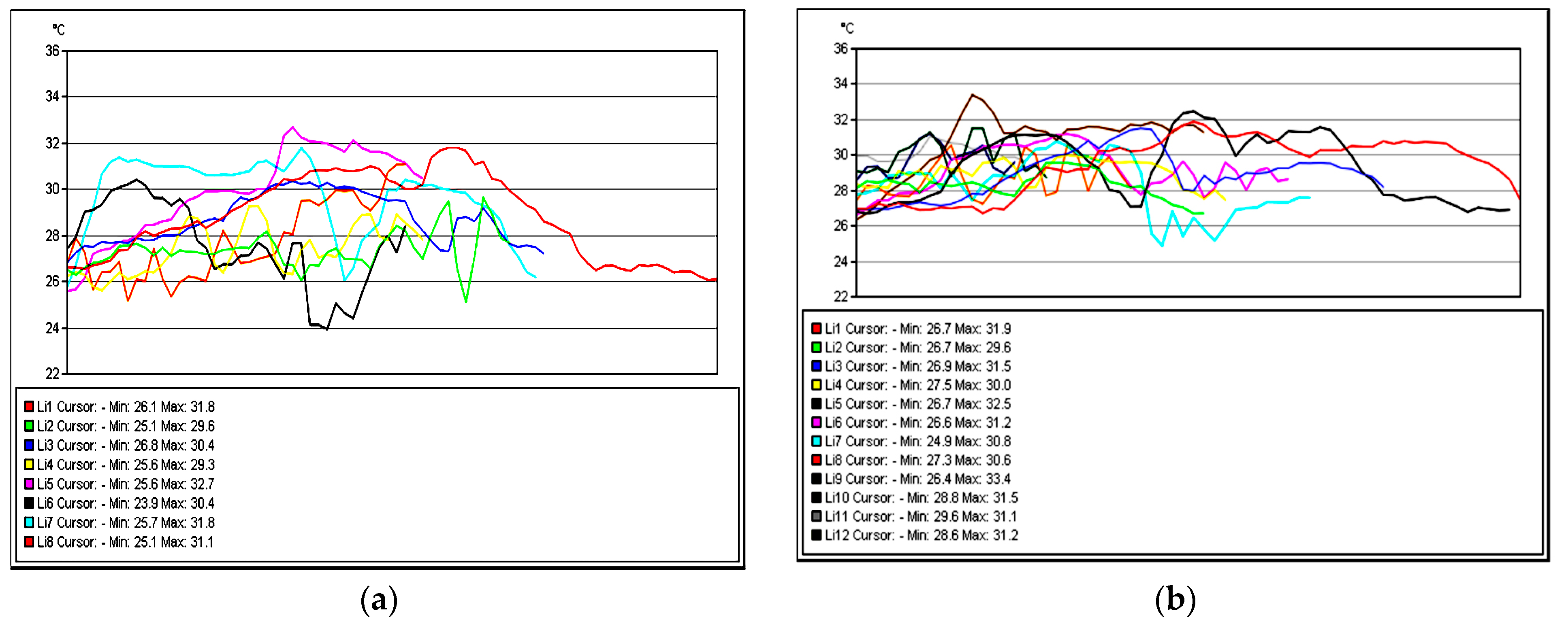
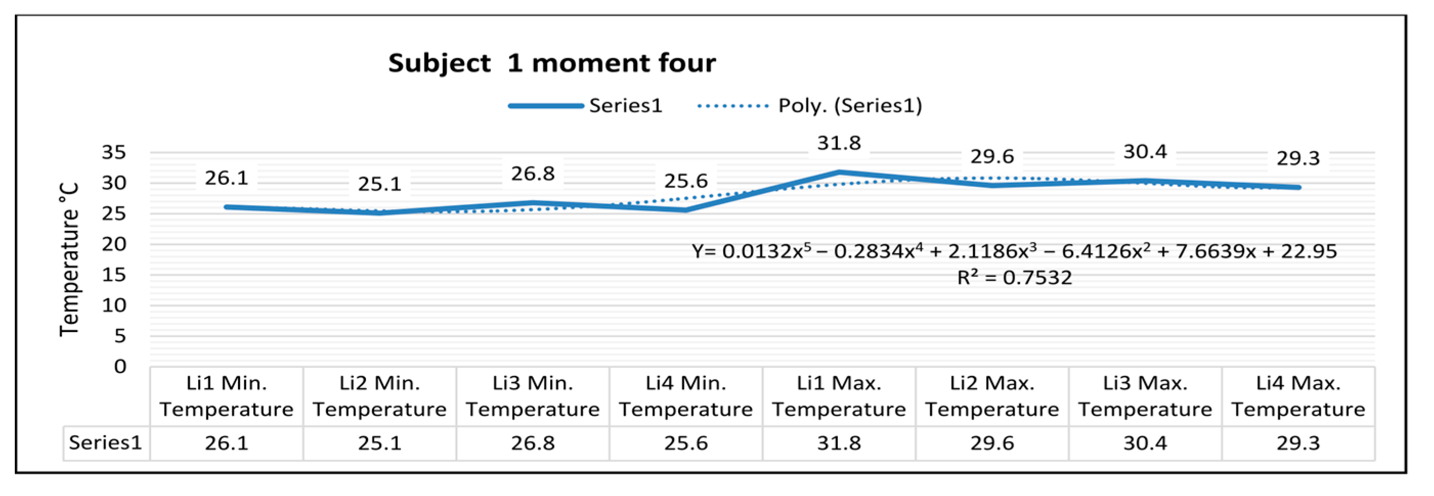
As shown in Figure 35, for the right foot of subject 1 at time four (at the end of volleyball training), the maximum temperature along the line Li1, which is positioned on the center of the foot, is 31.8 °C, and the minimum temperature is 26.1 °C. The temperature variation along the Li1 line is 5.7 °C, and the emissivity is 0.83 at time four. On the side along the Li2 line, the maximum temperature is 29.6 °C, and the minimum temperature is 25.1 °C at time four. The temperature variation along the Li2 line is 4.5 °C, and the emissivity is 0.83 at time four.
For the left foot of subject 1 at time four, the maximum temperature along the Li3 line positioned on the central side is 30.4 °C, and the minimum temperature is 26.8 °C. The temperature variation along the Li3 line is 3.5 °C, and the emissivity is 0.83, for subject 1 at time four. On the side along the Li4 line, the maximum temperature is 29.3 °C, and the minimum temperature is 25.6 °C, for subject 1 at time four. The temperature variation along the Li4 line is 3.7 °C, and the emissivity is 0.83, for subject 1 at time four.
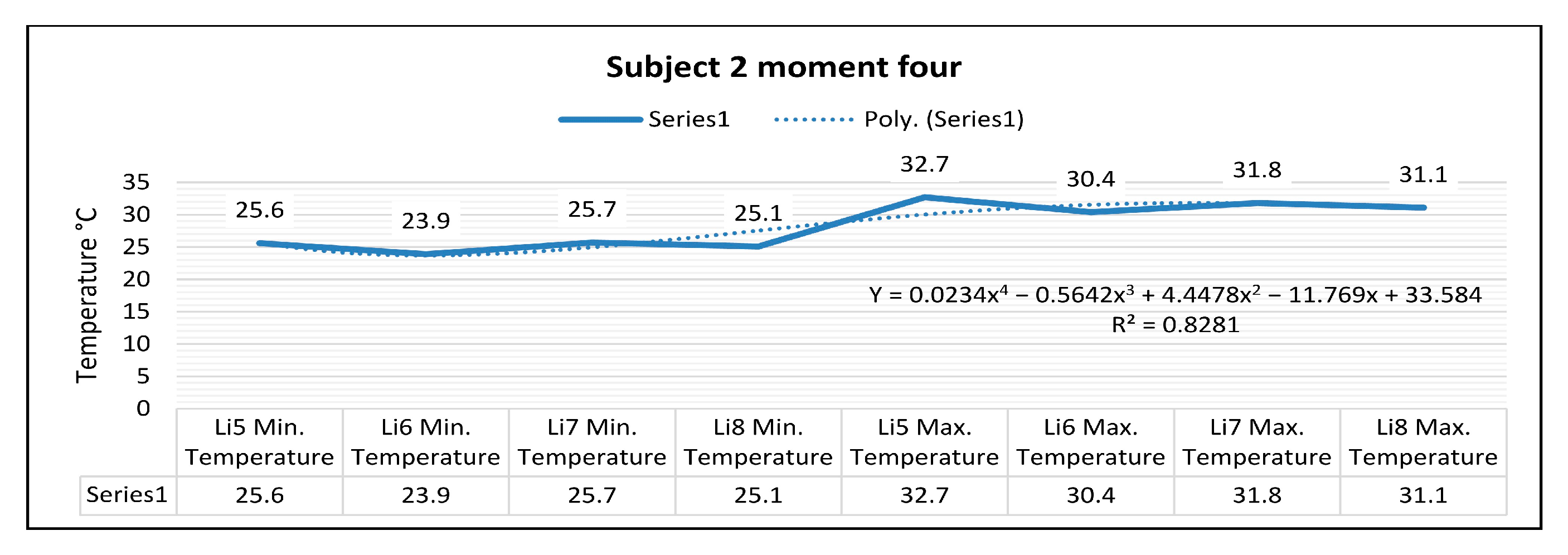
In Figure 35, for the right foot of subject 2 at time four (at the end of the volleyball training), the maximum temperature along the line Li5, which is positioned on the central part of the foot, is 32.7 °C, and the minimum temperature is 25.6 °C.
The temperature variation along the Li5 line is 7.1 °C, and the emissivity is 0.83 at time four. On the side along the Li6 line, the maximum temperature is 30.4 °C, and the minimum temperature is 23.9 °C at time four. The temperature variation along the Li6 line is 6.5 °C, and the emissivity is 0.83 at time four.
For the left foot of subject 2 at time four, the maximum temperature along the Li7 line positioned on the central side is 31.8 °C, and the minimum temperature is 25.7 °C.
The temperature variation along the Li7 line is 6.0 °C, and the emissivity is 0.83 at time four.
On the side along the Li8 line, the maximum temperature is 31.1 °C, and the minimum temperature is 25.1 °C at time four. The temperature variation along the Li8 line is 5.9 °C, and the emissivity is 0.83 at time four.
Thermography measurements afferent for subject 3 for the right foot at time four (at the end of volleyball training) show that the maximum temperature along the Li1 line, which is positioned on the center of the foot, is 30.8 °C, and the minimum temperature is 26.8 °C.
The temperature variation along the Li1 line is 4.0 °C, and the emissivity is 0.83 at time four. On the side along the Li2 line, the maximum temperature is 29.4 °C, and the minimum temperature is 26.7 °C at time four.
The temperature variation along the Li2 line is 2.7 °C, and the emissivity is 0.83 at time four.
For the left foot of subject 3 at time four, the maximum temperature along the Li3 line positioned on the central side is 30.9 °C, and the minimum temperature is 26.9 °C.
The temperature variation along the Li3 line is 3.9 °C, and the emissivity is 0.83 at time four.
On the side along the Li4 line, the maximum temperature is 30.0 °C, and the minimum temperature is 27.5 °C, at moment four. The temperature variation along the Li4 line is 2.5 °C, and the emissivity is 0.83 at time four.
In Figure 35, for the right foot of subject 4 at time four (at the end of volleyball training), the maximum temperature along the Li5 line, which is positioned on the center of the leg, is 32.5 °C, and the minimum temperature is 26.7 °C.
The temperature variation along the Li5 line is 5.8 °C, and the emissivity is 0.83 at time four. On the side along the Li6 line, the maximum temperature is 31.2 °C, and the minimum temperature is 26.6 °C at time four.
The temperature variation along the line is 4.6 °C, and the emissivity is 0.83 at time four. For the left foot of subject 4 at time four, the maximum temperature along the Li7 line positioned on the central side is 30.8 °C, and the minimum temperature is 24.9 °C.
The temperature variation along the Li7 line is 5.9 °C, and the emissivity is 0.83 at time four.
On the side along the Li8 line, the maximum temperature is 30.6 °C, and the minimum temperature is 27.3 °C at time four.
The temperature variation along the Li8 line is 3.3 °C, and the emissivity is 0.83 at time four.
In Figure 35, for the right foot of subject 5 at time four (at the end of the volleyball training), the maximum temperature along the line Li9, which is positioned on the central part of the foot, is 32.0 °C, and the minimum temperature is 25.8 °C.
The temperature variation along the Li9 line is 6.2 °C, and the emissivity is 0.83 at time four.
On the side along the Li10 line, the maximum temperature is 31.9 °C, and the minimum temperature is 27.2 °C at time four. The temperature variation along the Li10 line is 4.7 °C, and the emissivity is 0.83 at time four.
For the left foot of subject 5 at time four, the maximum temperature along the Li11 line positioned on the central side is 31.1 °C, and the minimum temperature is 29.6 °C.
The temperature variation along the Li11 line is 1.4 °C, and the emissivity is 0.83 at time four. On the side along the Li12 line, the maximum temperature is 31.2 °C, and the minimum temperature is 28.6 °C at time four.
The temperature variation along the Li12 line is 2.6 °C, and the emissivity is 0.83 at time four (at the end of the volleyball training).
Figure 36 shows the temperature variation along the subject lines on each footwear at time four.
In the case of subject 1 at time four, as shown in Figure 37, the relation obtained is a polynomial function of degree five (45).
Y = 0.0132x5 − 0.2834x4 + 2.1186x3 − 6.4126x2 + 7.6639x + 22.95
The coefficient of determining R2 established by the regression procedure is:
R2 = 0.7532
In the case of subject 2 at time four, as shown in Figure 38, the relation obtained is a polynomial function of degree four (47).
Y = 0.0234x4 − 0.5642x3 + 4.4478x2 − 11.769x + 33.584
The coefficient of determining R2 established by the regression procedure is:
R2 = 0.8281
In the case of subject 3 at time four, as shown in Figure 39, the relation obtained is a polynomial function of degree six (49).
Y = −0.0111x6 + 0.3057x5 − 3.2957x4 + 17.512x3 − 47.164x2 + 59.678x − 0.25
The coefficient of determining R2 established by the regression procedure is:
R2 = 0.9021
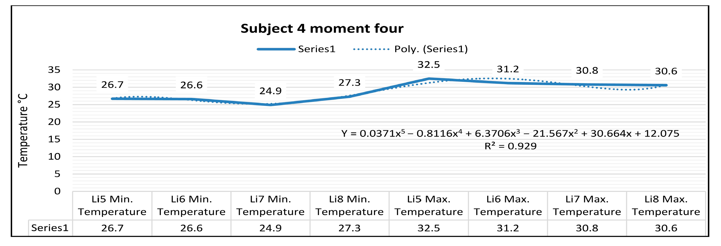
In the case of subject 4 at time four, as shown in Figure 40, the relation obtained is a polynomial function of degree five (51).
Y = 0.0371x5 − 0.8116x4 + 6.3706x3 − 21.567x2 + 30.664x + 12.075
The coefficient of determining R2 established by the regression procedure is:
R2 = 0.929
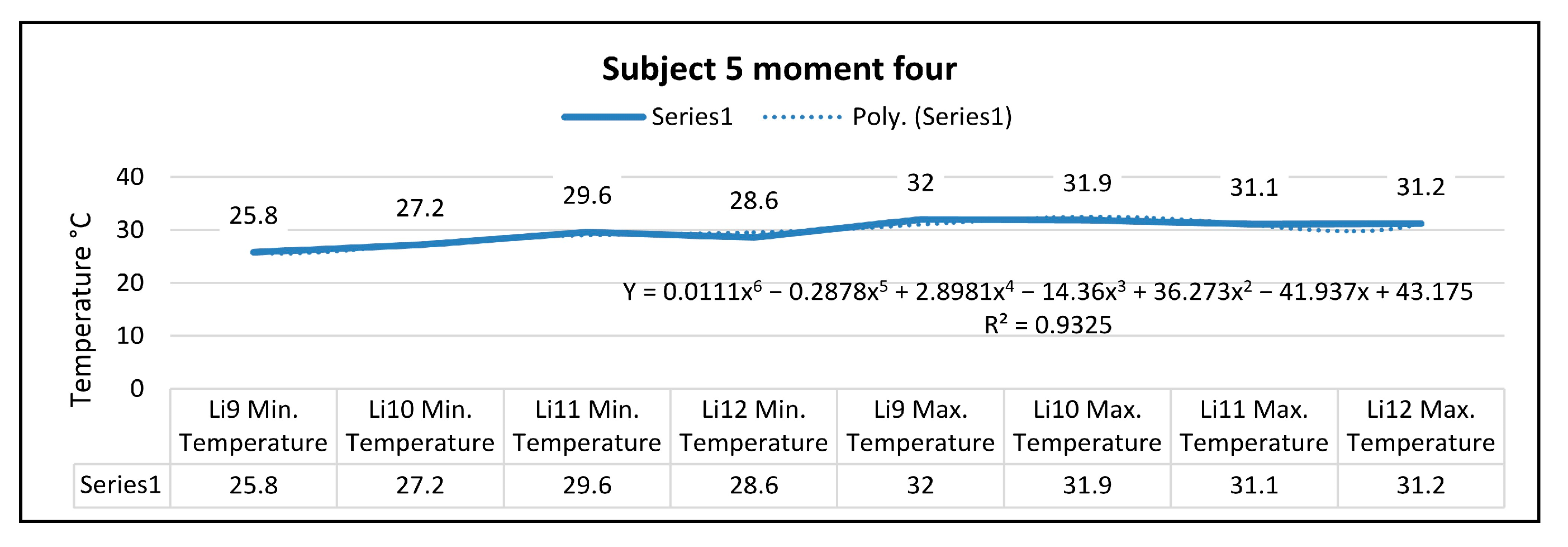
In the case of subject 5 at time four, as shown in Figure 41, the relation obtained is a polynomial function of degree six (53).
Y = 0.0111x6 − 0.2878x5 + 2.8981x4 − 14.36x3 + 36.273x2 − 41.937x + 43.175
The coefficient of determining R2 established by the regression procedure is:
R2 = 0.9325
Polynomial regression is used to create a mathematical model based on polynomials of degree four, five, and six by processing the experimental data and to predict the temperature values outside this range for each individual subject; this method is sensible because, based on the analysis of the polynomial type, a difference in the degree of the polynomial was observed when comparing the shoes of subjects 1 and 2 with the shoes of subjects 3, 4, 5.
It is observed from this analysis that for subjects 1 and 2, wearing the same type of footwear, the degree of the polynomials for moments one and two is the same (of degree five), and for moments zero, three, and four, the difference is small (of one degree between them).
For subject 3, the degree of the polynomials for moments zero and four is the same (of degree six), and for moments one, two, and three, the difference is small (of one degree between them).
For subject 4, the degree of the polynomials for moments zero, two, and three is the same (of degree six); it is also the same for moments one and four (of degree five).
For subject 5, the degree of the polynomials for moments zero, one, and two is the same (of degree 5); it is also the same for moments three and four (of degree six).
It can be seen from this analysis that the difference in the degrees of the polynomials from one shoe to the other is greater than the difference between them.
Considering that these analyses have been done by other researchers in the field in different settings, in research laboratories on unused sports footwear intended for indoor sports activities, the authors wanted to analyze whether there are significant differences in temperature distribution compared to those studied in laboratory conditions where the environment is much better controlled.
The authors studied indoor volleyball footwear in real time on several subjects during several volleyball training sessions to monitor the heat exchange between the foot and the outdoor environment at different times of training intensity, since most research is conducted in research laboratories [40].
The authors measured the variation in sports footwear temperature during volleyball training for the eight subjects analyzed, of which three subjects had a different model of the same sports footwear.
The analysis shows that the thermal distribution values are within the minimum and maximum limits of the five subjects analyzed in the paper, and they are presented in Table 3.
Sustainability in sports footwear includes many factors, such as design, supply chain, waste reduction, minimizing energy consumption, recycling, waste, and further innovation.
Based on the Young’s Modulus determined by 0.061 GPa for Asics sports footwear, it can be seen that the increase in temperature in the range of 23.1 °C–32.7 °C on the surface of the shoe influences the increase in Young’s modulus, which varies linearly with the increase in the temperature. Based on the Young’s Modulus determined by 0.039 GPa for Mizuno sports footwear, it can be observed that the temperature increase in the range of 23.1 °C–32.7 °C on the surface of the shoe influences the increase in Young’s modulus, which varies linearly with the increase in the temperature.
The polynomial regression is used to create a mathematical model based on processing the experimental data and to predict temperature values outside this domain.
In the mentioned cases when the regression of the polynomial function R2 has a value of less than 0.9, the mathematical model is less representative of the real situation, and the heat distribution on the analyzed surfaces of sports footwear is higher in the analyzed moments.
In the cases mentioned when the polynomial function regression R2 has a value higher than 0.9, the mathematical model represents the real situation, and the heat distribution on the analyzed areas of the sports footwear is higher.
In the case of subjects 1 and 2 using Asics footwear, it can be observed that the regression of the polynomial function R2 has a value of less than 0.9 at time zero (before starting the training). Following the measurements performed at time one (two minutes of training), only in the case of subject 2 did the regression of the polynomial function R2 have a value less than 0.9. In the case of time four (at the end of volleyball training), the regression of the polynomial function R2 had a value of less than 0.9 for subjects 1 and 2.
In the aforementioned cases, when the regression of the polynomial function R2 has a value of less than 0.9, the mathematical model is less representative of the real situation, and the heat distribution on the analyzed surfaces of sports footwear (Asics) is higher in the analyzed moments.
In the case of subjects 1 and 2 who use Asics sports footwear, there is an uneven distribution of temperature variation along the analyzed lines Li1, Li2, Li3, Li4, Li5, Li6, Li 7, and Li8 within the four moments in which the measurements were performed.
In the case of subjects 3, 4, and 5 who use Mizuno sports footwear, it can be observed that the polynomial function regression R2 has a value greater than 0.9 within the four moments analyzed.
In the cases mentioned when the polynomial function regression R2 has a value higher than 0.9, the mathematical model represents the real situation, and the heat distribution on the analyzed areas of the sports footwear (Mizuno) is higher only at moment four.
In the case of subjects 3, 4, and 5 who use Mizuno sports shoes, there is a uniform distribution of temperature variation along the analyzed lines Li1, Li2, Li3, Li4, Li5, Li6, Li 7, Li8, Li9, Li10, Li11, and Li12 during the four moments when the measurements were performed.
4. Conclusions

In the present paper, research was carried out in order to identify the thermal variation of indoor sports shoes used in volleyball training so as to detect the heat exchange between the foot and the outdoor environment.
Based on the values obtained from the research on the eight subjects, of which five subjects are relevant to this paper, we can conclude that the sole of the shoes is the coldest area, and for these reasons, we did not include these values in the data analysis, although subjects 3, 4, and 5 had footwear with ventilation in the sole, and the temperature distribution values were small in comparisons between them and subjects 1 and 2, whose soles were not ventilated (not significant).
The two pairs of footwear were exposed to the same temperature variations; one of the reasons why the heat transfer is different between the two models is due to the mechanical properties of the two materials, which are differentiated by their different Young’s modulus values.
Therefore, the test was valuable for showing the temperature distribution along the lines for each shoe and showing the strengths and weaknesses of the design of the tested footwear compared to the research done in the field. The authors conducted in the present research measurements from each angle of the room in which the volleyball training occurred, using a thermographic camera that was mounted on a tripod to capture the image in real time and from the same distance in static and dynamic moments.
Following the research and the data analyzed on sports footwear for the five tested subjects, it can be concluded that the sole of each shoe tested is the most insulating part, and the part that supports the heel shows the lowest heat transfer rates.
In future research, the variation in the Young’s modulus values can be examined at other temperatures analyzed in the present article, both on synthetic leather and on synthetic fibers.
The present research differs when compared to the majority of studies in the field, which are performed in a stationary configuration, despite the fact that it is well-known that the shoes of a real volleyball player are rarely stationary during training, where all the subsets are subjected to the same type of physical effort.
The authors of this paper aim to perform temperature measurements during a men’s volleyball training session to examine the distribution along temperature lines between subjects in the same environmental conditions and the advantages obtained by examining each shoe.

Author Contributions

Conceptualization, P.F.D., M.D.Ș., R.P. and S.D.B.; Methodology, M.D.Ș. and R.P.; Software, M.D.Ș. and R.P.; Formal analysis, S.D.B.; Data curation, M.D.Ș. and R.P.; Writing—original draft, P.F.D.; Writing — review & editing, M.D.Ș., R.P. and S.D.B.; Supervision, P.F.D. and S.D.B.; Funding acquisition, P.F.D. All authors have read and agreed to the published version of the manuscript.

Funding

The research was funded by the University of Oradea, within the Grants Competition “Scientific Research of Excellence Related to Priority Areas with Capitalization through Technology Transfer: INO–TRANSFER–UO”, Projects No. 238/2022.

Institutional Review Board Statement

The study was conducted in accordance with the Declaration of Helsinki and approved by the Ethics Committee of the University of Oradea.

Informed Consent Statement

Informed consent was obtained from all subjects involved in the study.

Data Availability Statement

The data presented in this study may be obtained on request from the corresponding author.

Acknowledgments

The FLIR SC 640 thermal imaging camera used in the research was acquired through a project of the Romanian–Hungarian R&D platform for intelligent building research projects supported by IntelBuild–HU-RO 0802/155. The research was made possible by the equal scientific contribution of all the authors concerned.
Conflicts of Interest

The authors declare no conflict of interest.

References

  1. Yick, K.I.; Annie, Y.; Ling, L.P. Insights into footwear preferences and insole design to improve thermal environment of footwear. Int. J. Fashion Design Tech. Ed. 2019, 12, 325–334. [Google Scholar] [CrossRef]
  2. West, A.M.; Oberst, F.; Tarrier, J.; Heyde, C.; Schlarb, H.; Brüggemann, G.-P.; Hodder, S.; Havenith, G. A thermal foot manikin as a tool for footwear evaluation and development. Proc. Inst. Mech. Eng. Part P J. S. Eng. Tech. 2020, 1, 1754337120952229. [Google Scholar] [CrossRef]
  3. Shimazaki, Y.; Matsutani, T.; Satsumoto, Y. Evaluation of thermal formation and air ventilation inside footwear during gait: The role of gait and fitting. Appl. Ergonom. 2016, 55, 234–240. [Google Scholar] [CrossRef]
  4. Bacter, C.; Săveanu, S.; Buhaș, R.; Marc, C. Housing for Sustainable Societies. Children’s Perception and Satisfaction with their House in Countries around the World. Sustainability 2021, 13, 8779. [Google Scholar] [CrossRef]
  5. Bacter, C.; Bălțătescu, S.; Marc, C.; Săveanu, S.; Buhaș, R. Correlates of Preadolescent Emotional Health in 18 Countries. A Study Using Children’s Words Data. Child Ind. Res. 2021, 14, 1703–1722. [Google Scholar] [CrossRef]
  6. Parsons, K.C. Protective clothing: Heat exchange and physiological objectives. Ergonomics 1988, 31, 991–1007. [Google Scholar] [CrossRef]
  7. Yu, A.N.; Li, P.L.; Yick, K.L.; Ng, S.P.; Yip, J.N. Investigation of Microclimate in Sports Shoes with the Integration of Human Subjective Sensations. Key Eng. Mater. 2018, 765, 140–146. [Google Scholar] [CrossRef]
  8. Miao, T.; Wang, P.; Zhang, N.; Li, Y. Footwear microclimate and its effects on the microbial community of the plantar skin. Sci. Rep. 2021, 11, 20356. [Google Scholar] [CrossRef]
  9. Ammer, K. Diagnosis of raynaud’s phenomenon by thermography. Skin Res. Tech. 2006, 2, 182–185. [Google Scholar] [CrossRef]
  10. Ng, E.Y.K.; Acharya, R. Remote-sensing infrared thermography. IEEE Eng. Med. Biol. 2009, 28, 76–83. [Google Scholar] [CrossRef]
  11. Tecklenburg, K.; Smekal, V.; Hoser, C.; Raschner, C.; El, A.R.; Fink, C. Incidence and injury mechanism of anterior cruciate ligament injury in professional junior alpine skiers in Austria. In Abstract-Book of the 12th European Society of Sports Traumatology Knee Surgery and Arthroscopy; ESSKA: Innsbruck, Austria, 23–27 May 2006; p. 159. [Google Scholar]
  12. Gold, J.E.; Cherniack, M.; Buchholz, B. Infrared thermography for examination of skin temperature in the dorsal hand of office workers. Eur. J. Appl. Physiol. 2004, 93, 245–251. [Google Scholar] [CrossRef]
  13. Kinoshita, H.; Bates, B.T. The effect of environmental temperature on the properties of running shoes. J. Appl. Biomech. 1996, 12, 258–268. [Google Scholar] [CrossRef]
  14. Kuklane, K. Protection of feet in cold exposure. Ind. Health 2009, 47, 242–253. [Google Scholar] [CrossRef] [PubMed] [Green Version]
  15. Yick, K.L.; Tang, K.P.M.; Li, P.L.; Yu, A.; Yip, J.; Ng, S.P. Instrumental Evaluation of Dry Heat Loss of Footwear under Different Activity Levels. IEEE Access 2019, 7, 65319–65331. [Google Scholar] [CrossRef]
  16. Shimazaki, Y.; Aisaka, K. Novel thermal analysis model of the foot-shoe sole interface during gait motion. Multidiscip. Digit. Publ. Inst. Proc. 2018, 2, 278. [Google Scholar]
  17. Mikhajlova, I.; Osina, T.; Prokhorov, V.; Mikhajlov, A. Mathematical model of the microclimate in shoes when exposed to low temperatures. Proc. High Sch. North Cauc. Reg. Tech. Sci. 2005, 2, 50–54. [Google Scholar]
  18. Ye, C.; Hang, H.; Fan, J.; Sun, W. Numerical Study of Heat and Moisture Transfer in Textile Materials by a Finite Volume Method. Commun. Comp. Phys. 2008, 4, 929–948. [Google Scholar]
  19. Buhaș, R.; Săveanu, S.; Bacter, C. Physical activity and other health related behaviors in adults from Oradea, Romania. Facts and social factors. Baltic J. Health Phys. Activ. 2020, 12, 36–45. [Google Scholar] [CrossRef]
  20. Georgescu, C.; Buhaș, R. Aspects regarding extracurricular sport activities in schools from Bihor County, Romania. Baltic J. of Health Physc. Act. 2020, 12, 69–78. [Google Scholar] [CrossRef]
  21. Olszewski-Strzyżowski, D.J.; Buhaș, R.; Buhaş, S. A sense of social affiliation of homeless people participating in a soccer tournament. Baltic J. Health Phys. Act. 2021, 13, 103–114. [Google Scholar] [CrossRef]
  22. Buhaș, S.; Buhaș, R.; Grama, V.; Herman, G.; Dragoș, P. The impact of local public policies on sports performance. Oradea–An example of success. Baltic J. Health Phys. Act. 2021, 13, 15–27. [Google Scholar] [CrossRef]
  23. Ilieș, D.C.; Buhaș, R.; Ilieș, M.; Ilieș, A.; Gaceu, O.; Pop, A.C.; Marcu, F.; Buhaș, S.D.; Gozner, M.; Baias, Ș. Sport activities and leisure in Nature 2000 protected area–Red Valley, Romania. J. Environ. Prot. Ecol. 2018, 19, 367–372. [Google Scholar]
  24. Ilieș, D.C.; Buhaș, R.; Ilieș, A.; Gaceu, O.; Oneț, A.; Buhaș, S.; Rahotă, D.; Dragoș, P.; Baiaș, Ș.; Marcu, F.; et al. Indoor air quality issues. Case study: The multipurpose sports hall of the University of Oradea. Environ. Eng. Manag. J. 2018, 17, 2999–3005. [Google Scholar]
  25. Gaceu, O.; Ilieș, D.C.; Baias, Ș.; Georgiță, M.; Ilieș, A.; Caciora, T.; Indire, L.; Albu, A.; Herman, G.V.; Baidog, A.; et al. Microclimatic characteristics and air quality inside the National Archives of Bihor county, Romania. Environ. Eng. Manag. J. 2021, 20, 459–466. [Google Scholar]
  26. Alcantara, E.; Artacho, M.A.; Gonzalez, J.C.; Garcia, A.C. Application of product semantics to footwear design. Part I—Identification of footwearsemantic space applying differential semantics. Int. J. Ind. Ergon. 2005, 35, 713–725. [Google Scholar] [CrossRef]
  27. Chang, C.A.; Lin, M.C.; Leonard, M.S.; Occena, L.G. Building an expert system for the design of sports shoes. Comput. Ind. Eng. 1988, 15, 72–77. [Google Scholar] [CrossRef]
  28. Shieh, M.D.; Yeh, Y.E. Developing a design support system for the exterior form of running shoes using partial least squares and neural networks. Comput. Ind. Eng. 2013, 65, 704–718. [Google Scholar] [CrossRef]
  29. Shieh, M.D.; Yeh, Y.E. Comparative study on perceptual evaluations of sports shoe exterior colors in Taiwan. Color Res. Appl. 2015, 40, 178–193. [Google Scholar] [CrossRef]
  30. Strangwood, M.; Subic, A. Modelling of materials for sports equipment. Mat. Sports Equip. 2007, 2, 3–34. [Google Scholar] [CrossRef]
  31. Chowdhury, H.; Alam, F.; Mainwaring, D.; Subic, A.; Tate, M.; Forster, D.; Beneyto-Ferre, J. Design and Methodology for Evaluating Aerodynamic Characteristics of Sports Textiles. Sport. Technol. 2009, 2, 81–86. [Google Scholar] [CrossRef]
  32. Chowdhury, H.; Alam, F.; Subic, A. Aerodynamic Performance Evaluation of Sports Textile. Proced. Eng. 2010, 2, 2517–2522. [Google Scholar] [CrossRef] [Green Version]
  33. Kyle, C.R.; Brownlie, L.W.; Harber, E.; MacDonald, R.; Norstrom, M. The Nike Swift Spin Cycling Project: Reducing the Aerodynamic Drag of Bicycle Racing Clothing by Using Zoned Fabrics. Eng. Sport 5 2004, 1, 118–124. [Google Scholar]
  34. Budzier, H.; Gerlach, G. Thermal Infrared Sensors: Theory, Optimisation and Practice; John Wiley & Sons: Chichester, UK, 2011; p. 328. ISBN 978-0-470-97675-3. [Google Scholar]
  35. Chua, J.H.J.; Dyer, A.G.; Garcia, J.E. Hot Shoes in the Room: Authentication of Thermal Imaging for Quantitative Forensic Analysis. J. Imaging 2018, 4, 21. [Google Scholar] [CrossRef] [Green Version]
  36. Maldague, X.P.V.; Jones, T.S.; Kaplan, H.; Marinetti, S.; Prystay, M. Chapter 2: Fundamentals of Infrared and Thermal Testing. In Nondestructive Handbook; ASNT Press: Columbus, OH, USA, 2001; pp. 26–137. [Google Scholar]
  37. Finney, A. Infrared photography. In The Focal Encyclopedia of Photography: Digital Imaging, Theory and Applications; History, and Science, Ed.; Elsevier/Focal Press: Burlington, NJ, USA, 2007; pp. 556–562. [Google Scholar]
  38. Puszkarz, A.K.; Usupov, A. The Study of Footwear Thermal Insulation Using Thermography and the Finite Volume Method. Int. J. Thermophys. 2019, 40, 1–14. [Google Scholar] [CrossRef] [Green Version]
  39. Stevenson, Christopher. Tutorial: Polynomial Regression in Excel. facultystaff. richmond. edu. Retrieved 22 January 2017. Available online: https://facultystaff.richmond.edu/~cstevens/301/Excel4.html (accessed on 14 March 2022).
  40. Dessing, O.; Jansen, A.J.; Leihitu, C.; Overhage, D. Experimental Study of Heat Dissipation in Indoor Sports Shoes. Proced. Eng. 2014, 72, 14–17. [Google Scholar] [CrossRef] [Green Version]
  41. Covill, D.; Guan, Z.W.; Bailey, M.; Raval, H. Development of thermal models of footwear using finite element analysis. Proc. Inst. Mech. Eng. Part H J. Eng. Med. 2011, 225, 268–281. [Google Scholar] [CrossRef] [PubMed]
  42. ISO 14577-1:2015; Metallic Materials—Instrumented Indentation Test for Hardness and Materials Parameters—Part 1: Test Method. International Organization for Standardization: Geneva, Switzerland, 2015.
  43. Singh, J.I.P.; Singh, S.; Dhawan, V. Effect of Curing Temperature on Mechanical Properties of Natural Fiber Reinforced Polymer Composites. J. Nat. Fibers 2018, 15, 687–696. [Google Scholar] [CrossRef]
Figure 1. FLIR 640 thermal imaging camera components.
Sustainability 15 00652 g001
Figure 2. Thermography measurements on 8 subjects during volleyball training.
Sustainability 15 00652 g002
Figure 3. IR and real spectrum image of the five subjects: (a) infrared image, (b) real image.
Sustainability 15 00652 g003
Figure 4. Footwear image and material characteristics for Asics and Mizuno: (a) Material characteristics for Asics, synthetic fiber with synthetic leather upper/rubber sole, (b) material characteristics for Mizuno, synthetic fiber with synthetic leather upper/rubber sole.
Sustainability 15 00652 g004
Figure 5. Temperature influence on the evolution of Young’s modulus for Asics footwear.
Sustainability 15 00652 g005
Figure 6. Temperature influence on the evolution of Young’s modulus for Mizuno footwear.
Sustainability 15 00652 g006
Figure 7. Variation of sports footwear temperature at time zero on the 5 subjects: (a) subjects 1 and 2 in infrared; (b) subjects 3, 4, 5 in infrared.
Sustainability 15 00652 g007
Figure 8. Temperature variation along the lines positioned on sports footwear at time zero: (a) temperature variation along the lines for subjects 1 and 2, (b) temperature variation along the lines for subjects 3, 4, 5.
Sustainability 15 00652 g008
Figure 9. Temperature variation on sports footwear for subject 1 at time zero.
Sustainability 15 00652 g009
Figure 10. Temperature variation on sports footwear for subject 2 at time zero.
Sustainability 15 00652 g010
Figure 11. Temperature variation on sports footwear for subject 3 at time zero.
Sustainability 15 00652 g011
Figure 12. Temperature variation on sports footwear for subject 4 at time zero.
Sustainability 15 00652 g012
Figure 13. Temperature variation on sports footwear for subject 5 at time zero.
Sustainability 15 00652 g013
Figure 14. Variation of sports footwear temperature at time one on the 5 subjects: (a) subjects 1 and 2 in infrared, (b) subjects 3, 4, 5 in infrared.
Sustainability 15 00652 g014
Figure 15. Temperature variation along the lines positioned on sports footwear at time one: (a) temperature variation along the lines for subjects 1 and 2, (b) temperature variation along the lines for subjects 3, 4, 5.
Sustainability 15 00652 g015
Figure 16. Temperature variation on sports footwear for subject 1 at time one.
Sustainability 15 00652 g016
Figure 17. Temperature variation on sports footwear for subject 2 at time one.
Sustainability 15 00652 g017
Figure 18. Temperature variation on sports footwear for subject 3 at time one.
Sustainability 15 00652 g018
Figure 19. Temperature variation on sports footwear for subject 4 at time one.
Sustainability 15 00652 g019
Figure 20. Temperature variation on sports footwear for subject 5 at time one.
Sustainability 15 00652 g020
Figure 21. Variation of sports footwear temperature at time two on the 5 subjects: (a) subjects 1 and 2 in infrared, (b) subjects 3, 4, 5 in infrared.
Sustainability 15 00652 g021
Figure 22. Temperature variation along the lines positioned on sports footwear at time two: (a) temperature variation along the lines for subjects 1 and 2, (b) temperature variation along the lines for subjects 3, 4, 5.
Sustainability 15 00652 g022
Figure 23. Temperature variation on sports footwear for subject 1 at time two.
Sustainability 15 00652 g023
Figure 24. Temperature variation on sports footwear for subject 2 at time two.
Sustainability 15 00652 g024
Figure 25. Temperature variation on sports footwear for subject 3 at time two.
Sustainability 15 00652 g025
Figure 26. Temperature variation on sports footwear for subject 4 at time two.
Sustainability 15 00652 g026
Figure 27. Temperature variation on sports footwear for subject 5 at time two.
Sustainability 15 00652 g027
Figure 28. Variation of sports footwear temperature at time three on the 5 subjects: (a) subjects 1 and 2 in infrared, (b) subjects 3, 4, 5 in infrared.
Sustainability 15 00652 g028
Figure 29. Temperature variation along the lines positioned on sports footwear at time three: (a) temperature variation along the lines for subjects 1 and 2, (b) temperature variation along the lines for subjects 3, 4, 5.
Sustainability 15 00652 g029
Figure 30. Temperature variation on sports footwear for subject 1 at time three.
Sustainability 15 00652 g030
Figure 31. Temperature variation on sports footwear for subject 2 at time three.
Sustainability 15 00652 g031
Figure 32. Temperature variation on sports footwear for subject 3 at time three.
Sustainability 15 00652 g032
Figure 33. Temperature variation on sports footwear for subject 4 at time three.
Sustainability 15 00652 g033
Figure 34. Temperature variation on sports footwear for subject 5 at time three.
Sustainability 15 00652 g034
Figure 35. Variation of sports footwear temperature at time four on the 5 subjects: (a) subjects 1 and 2 in infrared, (b) subjects 3, 4, 5 in infrared.
Sustainability 15 00652 g035
Figure 36. Temperature variation along the lines positioned on sports footwear at time four: (a) temperature variation along the lines for subjects 1 and 2, (b) temperature variation along the lines for subjects 3, 4, 5.
Sustainability 15 00652 g036
Figure 37. Temperature variation in sports footwear for subject 1 at time four.
Sustainability 15 00652 g037
Figure 38. Temperature variation in sports footwear for subject 2 at time four.
Sustainability 15 00652 g038
Figure 39. Temperature variation in sports footwear for subject 3 at time four.
Sustainability 15 00652 g039
Figure 40. Temperature variation in sports footwear for subject 4 at time four.
Sustainability 15 00652 g040
Figure 41. Temperature variation in sports footwear for subject 5 at time four.
Sustainability 15 00652 g041
Table 1. Mechanical proprieties for Asics footwear.
TestModulus at Max Load
GPa
Hardness at Max Load
GPa
Drift Correction
Nm/s
Displacement at Max Load
Nm
Load at Max Load
mN
Mean0.0610.007−0.4172084.760.348
Standard Deviation0.0180.0050.22377.110.193
% Coefficient of Variation46.9566.63−53.473.755.57
Table 2. Mechanical proprieties for Mizuno footwear.
TestModulus at Max Load
GPa
Hardness at Max Load
GPa
Drift Correction
Nm/s
Displacement
at Max Load
Nm
Load at Max Load
mN
Mean0.0390.01−0.1982115.8560.495
Standard Deviation0.0160.0060.33530.3820.184
% Coefficient of Variation26.4662.13−169.171.4437.24
Table 3. Variation of the sports footwear temperature during volleyball training at the time of measurements for the 5 selected subjects from 8 analyzed.
SubjectTime ZeroTime OneTime TwoTime ThreeTime Four
Subject 1Li1 max 28.1 °CLi1 max 28.9 °CLi1 max 29.0 °CLi1 max 30.6 °CLi1 max 31.8 °C
Li1 min 23.8 °CLi1 min 22.3 °CLi1 min 22.1 °CLi1 min 25.4 °CLi1 min 26.1 °C
Li2 max 26.6 °CLi2 max 29.6 °CLi2 max 30.1 °CLi2 max 30.4 °CLi2 max 29.6 °C
Li2 min 23.1 °CLi2 min 22.8 °CLi2 min 22.5 °CLi2 min 23.7 °CLi2 min 25.1 °C
Li3 max 28.4 °CLi3 max 28.3 °CLi3 max 28.9 °CLi3 max 30.1 °CLi3 max 30.4 °C
Li3 min 23.2 °CLi3 min 23.6 °CLi3 min 23.5 °CLi3 min 23.2 °CLi3 min 26.8 °C
Li4 max 27.3 °CLi4 max 27.2 °CLi4 max 29.5 °CLi4 max 29.0 °CLi4 max 29.3 °C
Li4 min 24.0 °CLi4 min 22.9 °CLi4 min 23.0 °CLi4 min 23.5 °CLi4 min 25.6 °C
Subject 2Li5 max 29.1 °CLi5 max 30.1 °CLi5 max 29.6 °CLi5 max 31.3 °CLi5 max 32.7 °C
Li5 min 24.9 °CLi5 min 24.0 °CLi5 min 23.3 °CLi5 min 27.1 °CLi5 min 25.6 °C
Li6 max 28.5 °CLi6 max 28.9 °CLi6 max 31.4 °CLi6 max 31.6 °CLi6 max 30.4 °C
Li6 min 24.5 °CLi6 min 23.9 °CLi6 min 25.8 °CLi6 min 26.6 °CLi6 min 23.9 °C
Li7 max 28.2 °CLi7 max 28.8 °CLi7 max 30.6 °CLi7 max 30.9 °CLi7 max 31.8 °C
Li7 min 24.8 °CLi7 min 23.6 °CLi7 min 25.5 °CLi7 min 23.8 °CLi7 min 25.7 °C
Li8 max 27.8 °CLi8 max 28.1 °CLi8 max 29.7 °CLi8 max 31.3 °CLi8 max 31.1 °C
Li8 min 23.6 °CLi8 min 23.5 °CLi8 min 24.9 °CLi8 min 26.6 °CLi8 min 25.1 °C
Subject 3Li1 max 27.1 °CLi1 max 28.6 °CLi1 max 29.5 °CLi1 max 31.3 °CLi1 max 30.8 °C
Li1 min 22.9 °CLi1 min 23.4 °CLi1 min 23.0 °CLi1 min 25.9 °CLi1 min 26.8 °C
Li2 max 26.1 °CLi2 max 27.9 °CLi2 max 27.5 °CLi2 max 30.2 °CLi2 max 29.4 °C
Li2 min 25.0 °CLi2 min 22.9 °CLi2 min 22.5 °CLi2 min 26.1 °CLi2 min 26.7 °C
Li3 max 27.0 °CLi3 max 27.6 °CLi3 max 29.0 °CLi3 max 30.4 °CLi3 max 30.9 °C
Li3 min 24.0 °CLi3 min 22.4 °CLi3 min 23.5 °CLi3 min 25.4 °CLi3 min 26.9 °C
Li4 max 26.1 °CLi4 max 26.6 °CLi4 max 27.7 °CLi4 max 30.2 °CLi4 max 30.0 °C
Li4 min 24.1 °CLi4 min 23.8 °CLi4 min 25.2 °CLi4 min 26.5 °CLi4 min 27.5 °C
Subject 4Li5 max 26.7 °CLi5 max 26.4 °CLi5 max 29.5 °CLi5 max 31.0 °CLi5 max 32.5 °C
Li5 min 23.2 °CLi5 min 22.3 °CLi5 min 23.6 °CLi5 min 24.2 °CLi5 min 26.7 °C
Li6 max 25.5 °CLi6 max 26.1 °CLi6 max 27.0 °CLi6 max 29.6 °CLi6 max 31.2 °C
Li6 min 23.1 °CLi6 min 22.6 °CLi6 min 23.2 °CLi6 min 25.8 °CLi6 min 26.6 °C
Li7 max 25.9 °CLi7 max 26.7 °CLi7 max 27.7 °CLi7 max 29.5 °CLi7 max 30.8 °C
Li7 min 23.0 °CLi7 min 22.0 °CLi7 min 22.6 °CLi7 min 24.1 °CLi7 min 24.9 °C
Li8 max 25.4 °CLi8 max 25.9 °CLi8 max 27.4 °CLi8 max 29.4 °CLi8 max 30.6 °C
Li8 min 24.0 °CLi8 min 22.2 °CLi8 min 22.5 °CLi8 min 25.0 °CLi8 min 27.3 °C
Subject 5Li9 max 27.9 °CLi9 max 28.3 °CLi9 max 30.0 °CLi9 max 31.9 °CLi9 max 32.0 °C
Li9 min 23.7 °CLi9 min 23.0 °CLi9 min 23.3 °CLi9 min 23.8 °CLi9 min 25.8 °C
Li10 max 27.0 °CLi10 max 28.0 °CLi10 max 28.0 °CLi10 max 30.5 °CLi10 max 31.9 °C
Li10 min 24.6 °CLi10 min 23.0 °CLi10 min 23.0 °CLi10 min 25.9 °CLi10 min 27.2 °C
Li11 max 26.0 °CLi11 max 26.7 °CLi11 max 28.3 °CLi11 max 29.5 °CLi11 max 31.1 °C
Li11 min 22.8 °CLi11 min 22.9 °CLi11 min 23.2 °CLi11 min 27.3 °CLi11 min 29.6 °C
Li12 max 26.2 °CLi12 max 27.0 °CLi12 max 26.5 °CLi12 max 29.9 °CLi12 max 31.2 °C
Li12 min 24.7 °CLi12 min 23.3 °CLi12 min 22.6 °CLi12 min 27.1 °CLi12 min 28.6 °C
Disclaimer/Publisher’s Note: The statements, opinions and data contained in all publications are solely those of the individual author(s) and contributor(s) and not of MDPI and/or the editor(s). MDPI and/or the editor(s) disclaim responsibility for any injury to people or property resulting from any ideas, methods, instructions or products referred to in the content.