Article

Research on Vehicle Active Steering Stability Control Based on Variable Time Domain Input and State Information Prediction

1
China North Vehicle Research Institute, Beijing 100072, China
2
Beijing University of Civil Engineering and Architecture, Beijing 100044, China
3
China North Artificial Intelligence & Innovation Research Institute, Beijing 100072, China
4
Beijing Institute of Technology, Beijing 100081, China
*
Author to whom correspondence should be addressed.
Sustainability 2023, 15(1), 114; https://doi.org/10.3390/su15010114
Submission received: 14 November 2022 / Revised: 9 December 2022 / Accepted: 14 December 2022 / Published: 21 December 2022

Abstract

:
The controller design of vehicle systems depends on accurate reference index input. Considering information fusion and feature extraction based on existing data settings in the time domain, if reasonable input is selected for prediction to obtain accurate information of future state, it is of great significance for control decision-making, system response, and driver’s active intervention. In this paper, the nonlinear dynamic model of the four-wheel steering vehicle system was built, and the Long Short-Term Memory (LSTM) network architecture was established. On this basis, according to the real-time data under different working conditions, the information correction calculation of variable time-domain length was carried out to obtain the real-time state input length. At the same time, the historical state data of coupled road information was adopted to train the LSTM network offline, and the acquired real-time data state satisfying the accuracy was used as the LSTM network input to carry out online prediction of future confidence information. In order to solve the problem of mixed sensitivity of the system, a robust controller for vehicle active steering was designed with the sideslip angle of the centroid of 0, and the predicted results were used as reference inputs for corresponding numerical calculation verification. Finally, according to the calculated results, the robust controller with information prediction can realize the system stability control under coupling conditions on the premise of knowing the vehicle state information in advance, which provides an effective reference for controller response and driver active manipulation.

1. Introduction

With the continuous development of multi-sensor fusion technology [1], wire chassis technology [2], and brain-inspired intelligence technology [3], vehicle chassis system control is gradually changing from expected control of single performance to synchronous optimization of multiple performances. The following is the overall optimization of system performance under the control of multiple subsystems. The degree of information interaction, the depth of data fusion [4], and the requirements for intelligent parameter identification under big data are also constantly improved in this process [5].
In intelligent transportation and information network, whether for traditional vehicles or autonomous vehicles, the determination, decision, and control of vehicle stability are not only dependent on a single sensor or signal source [6] but also related to multiple states at the current time and signal information at multiple times [7]. If the future behavior or states of the vehicle can be reasonably predicted with the help of current information, it will help the vehicle avoid unknown risks in complex environments and make decisions on corresponding hazards for early intervention and active control [8]. The full-state observer could be employed to predict the rollover risk of vehicles traveling on sloping roads based on information including longitudinal speed, lateral acceleration, and suspension displacement [9]. The two-level quantization adaptive Kalman filtering algorithm incorporating the autoregressive moving average model was applied in the vehicle networking system to achieve the vehicle state prediction in the traffic network based on shared state information [10]. According to the driver’s manipulation behavior, the cumulative calculation of energy consumption up to the current moment could be realized, thus a specific energy consumption analysis and prediction model independent of the vehicle model was proposed, which could achieve the prediction of system energy consumption and future vehicle speed [11]. In addition, based on the data information interaction process between vehicles in the traffic network, an active traffic safety management system was developed to predict future vehicle behavior using past information, promptly conduct risk judgment, and put forward warning information [12]. The interaction information between vehicles is helpful to identify vehicle behavior. Combined with the prediction results of vehicle state information, an accurate vehicle driving track can be obtained [13].
Meanwhile, this paper adopts the four-wheel active steering system combined with the chassis by wire technology and real-time states update as the control object, which uses the motor as the active steering actuator to actively correct the steering angle of the front/rear wheels in real-time. During the handling and driving process, the rotation direction of the front/rear wheels can be dynamically adjusted according to external needs [14]. Compared with the front/rear wheel active steering system, the four-wheel active steering system, which worked in coordination with the electronic control unit, had a faster response speed. Furthermore, it could effectively reduce the turning radius during steering, and maintain good handling stability in the process of fast cornering [15]. Through the real-time calculation of tracking yaw rate error in the process of vehicle active steering, the actual error value would be input into the PI controller so that front/rear wheel steering could be combined to achieve linear dynamic eigenvalue distribution without lateral speed measurement [16]. The second-order decoupling controller, which was designed by adding the additional steering angle of the wheel as the control input, could decouple the correlation between vehicle yaw rate and lateral speed [17]. On this foundation, the input of the sideslip angle of the vehicle centroid was further considered, and the joint feedback of the sideslip angle and yaw rate could be used to conduct robust control of the vehicle’s active steering process [18]. In order to eliminate the chatter of the discontinuous system and ensure system convergence in the finite time domain, a novel non-smooth finite time domain control method was proposed to satisfy the target requirements of zero centroid sideslip angle and ideal yaw rate [19]. The combined application of independent steering technology and driving technology could optimize the tire force distribution online to achieve active fault tolerant control of the system under external disturbance and system fault reconstruction conditions [20]. Through multi-source excitation decomposition and combining the natural frequency analysis with the vehicle steering system, an effective reference for the structural design of the steering system can be provided [21,22].
Although there has been in-depth research on state information fusion prediction [23] and chassis active integrated control [24], further exploration and verification are still needed for corresponding deficiencies. In the case of external input and excitation disturbance, whether the prediction of the target vehicle state can be acquired also requires investigation [25]. On the other hand, on the premise of obtaining existing data and conducting adequate training, how to realize vehicle stability robust control based on the online prediction of artificial intelligence algorithm data has become a scientific question that needs further research. In order to achieve vehicle stability control based on vehicle confidence state prediction information in the time domain, an integration method combining variable time domain state input LSTM network and mixed sensitivity robust controller is proposed. This method dynamically corrects the input state length of the LSTM network at the current time through real-time error feedback and then obtains the confidence output as the control input of the robust controller to realize the research of front and rear wheel coordinated control strategy in the process of vehicle active steering.
In summary, the research framework of this paper is listed as follows: in Section 2, the vehicle dynamics model based on the system nonlinear characteristics including body roll and nonlinear lateral force is built; on this basis, the time domain length calculation of the input state considering both data length and calculation accuracy is implemented, and the LSTM network integrating variable time-domain length input is set up in Section 3; then, the robust controller design based on the mixed sensitivity problem of the system is designed in Section 4; Section 5 discusses the numerical calculation results under different driving conditions; finally, the relevant conclusions are summarized in Section 6.

2. Nonlinear Vehicle Dynamics Model

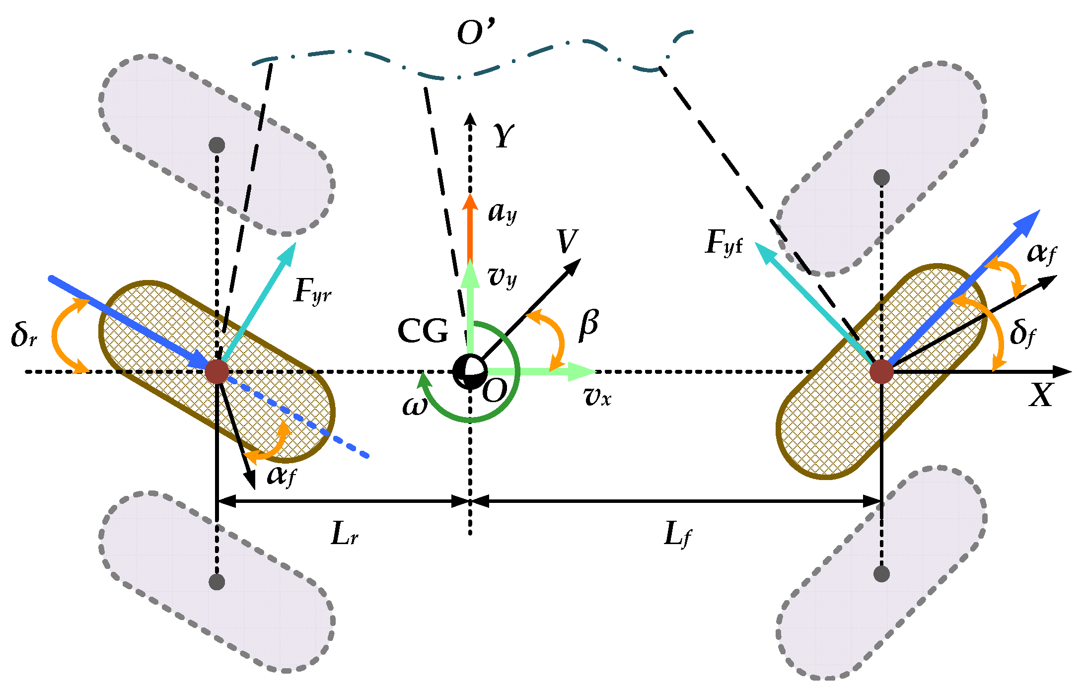
Based on the four-wheel active steering system, the nonlinear system modeling of vehicle longitudinal, lateral, and body motion is carried out in this paper. Among them, the active steering process of the front and rear wheels mainly provides the wheel angle correction value by actively controlling the current of the steering motor to ensure the vehicle’s safety and system stability during the steering operation. The specific physical vehicle model is shown in Figure 1.
Considering the longitudinal motion, lateral motion and yaw motion at the vehicle centroid [26], the following system dynamics equation can be built:
m a x = F x f l cos δ f l + F x f r cos δ f r F y f l sin δ f l F y f r sin δ f r + F x r l cos δ r l + F x r r cos δ r r F y r l sin δ r l F y r r sin δ r r m g sin θ 1 2 C d A d ρ v x 2
m a y = F x f l sin δ f l + F x f r sin δ f r + F y f l cos δ f l + F y f r cos δ f r F x r l sin δ r l F x r r sin δ r r + F y r l cos δ r l + F y r r cos δ r r + m g sin φ
I z ω ˙ = L f F x f l sin δ f l + F x f r sin δ f r + F y f l cos δ f l + F y f r cos δ f r L r F x r l sin δ r l F x r r sin δ r r + F y r l cos δ r l + F y r r cos δ r r B f l F x f l cos δ f l F y f l s i n δ f l B r l F x r l cos δ r l F y r l s i n δ r l + B r l F x f r cos δ f r F y f r sin δ f r + B r r F x r r cos δ r r F y r r sin δ r r + ω d
where ax and ay are the longitudinal acceleration and lateral acceleration of the vehicle, respectively, Fxi and Fyi (i = fl, fl, rl, rr) are the longitudinal force and lateral force of the wheel, respectively, δi (i = fl, fl, rl, rr) is the tire steering angle, m is the vehicle mass, g is the acceleration of gravity, Cd is the air resistance coefficient, Ad is the equivalent wind resistance area, ρ is the air density, θ and φ are pitch angle and roll angle of the vehicle body, respectively, ω and ωd are the vehicle body yaw rate and its torque disturbance value, respectively, Lf and Lr are the distances from the vehicle centroid to the front axle and rear axle, respectively, Bi (i = fl, fl, rl, rr) is the lateral distance between the centroid and the corresponding tire, and Iz is the moment of inertia of the vehicle about the Z-axis.
Assuming that the longitudinal driving speed (vx) at the vehicle centroid remains constant, and considering the body roll motion during steering [27], the four tire sideslip angles of the vehicle are exhibited as follows:
α f l = arctan v y   +   L f ω v x     B f l ω δ f l ψ f φ ,   α f r = arctan v y   +   L f ω v x   +   B f r ω δ f r ψ f φ α r l = arctan v y     L r ω v x     B r l ω δ r l ψ r φ ,   α f r = arctan v y     L r ω v x   +   B r r ω δ r r ψ r φ
where ψf and ψr are the system steering coefficients of the front and rear axles of the vehicle in the steering process, respectively.
The Newton–Euler equation is adopted to model the body roll motion. Assuming that Bfl = Bfr = Brl = Brr = B, the nonlinear calculation formula of vehicle roll acceleration is given according to the rate of change of angular momentum as follows:
φ ¨ = m a y H R cos φ   +   m g H R sin φ     C R φ ˙     K R φ   +   ω 2 I y     I z φ I x   +   m b B tan φ   +   B 2 sin 2 φ   +   4 H R 2 2 m a y H R   +   m g H R   +   ω 2 I y     I z     K R φ     C R φ ˙ I x   +   m b B φ   +   B 2 φ 2   +   4 H R 2 2
where HR is the roll center height of the vehicle.
The sideslip angle at the vehicle centroid corresponds to:
β = arctan v y v x
In addition, in the process of lateral force calculation, to avoid the tedious calculation caused by the magic tire formula, under the assumption that the sideslip angles of the left and right tires on the same axis of the vehicle are approximately equal, the TS vehicle tire model considering the nonlinear characteristics of the tires is introduced to calculate the corresponding lateral forces of the wheels [28]. Assuming that the sideslip angles of the front and rear tires of the vehicle are αf and αr, the lateral force of the front and rear axles of the vehicle has the following corresponding relationship:
F y f = χ 1 α f C f 1 α f + χ 2 α f C f 2 α f F y r = χ 1 α f C f 1 α r + χ 2 α f C f 2 α r
where χi (i = 1, 2) is the membership function, which can be calculated according to the following formula:
χ i α f = Λ i α f i = 1 2 Λ i α f Λ i α f = 1 1 + α f x i y i 2 z i   ,   i = 1 , 2
In the above formula, xi, yi, and zi are the membership function parameters, respectively, which can be obtained through the joint calculation of the Levenberg–Marquardt algorithm and the least squares algorithm.
Considering the dynamic changes of the vehicle body during driving, the vertical dynamic loads at the four tires of the vehicle can be calculated as follows:
F z f l = m g   +   a z L r     H R sin θ     m a x H C 2 L f   +   L r m a y H C L r     H R sin θ 2 B f l L f   +   L r α z f r = m g   +   a z L r     H R sin θ     m a x H C 2 L f   +   L r + m a y H C L r     H R sin θ 2 B f r L f   +   L r α z r l = m g   +   a z L f     H R sin θ   +   m a x H C 2 L f   +   L r m a y H C L f   +   H R sin θ 2 B r l L f   +   L r α z f r = m g   +   a z L f     H R sin θ   +   m a x H C 2 L f   +   L r + m a y H C L f   +   H R sin θ 2 B r r L f   +   L r
where HC is the vertical height between the vehicle centroid and the ground, and its dynamic calculation method is:
H C = H R + H C R cos θ sin φ
where HCR is the distance between the vehicle centroid and the vehicle roll center.
Therefore, by further considering the influence of vertical load on the lateral force, the lateral force of the vehicle tire corresponding to the sideslip angle under different vertical dynamic loads can be obtained as shown in Figure 2 below. The data in Figure 2 are the tire lateral force characteristics of the research object with the corresponding sideslip angle and vertical load in the range of 0–23,000 N. According to the data curves, the tire lateral force characteristics of the vehicle under different working conditions can be obtained.
In the static state, the vehicle load is constant. However, during driving, body movements such as pitching and rolling will lead to changes in the vertical dynamic loads of different tires, so the corresponding tire lateral forces will also change. The vehicle tire model shown in Figure 2 can adapt to the engineering application and calculation of the nonlinear lateral force of vehicle tires, which provides great convenience for online calculation of the model.
In order to avoid steering wheel jitter induced by small external disturbances at high speed, the dead zone range of the steering wheel angle is set. Only when the steering wheel angle of the vehicle is outside the dead zone, the proportion differentiation (PD) controller is employed to actively control the high-speed steering sensitivity of the front and rear wheels of the vehicle based on the steering wheel angle [29], and its corresponding control currents IC_f and IC_r are as follows:
I C _ f = k f p δ s + k f d δ ˙ s I C _ r = k r p δ s + k r d δ ˙ s
where kfp and kfd are respectively the proportion and differential coefficients of the steering wheel angle relative to the front wheel control current, and krp and krd are respectively the proportion and differential coefficients of the steering wheel angle relative to the rear wheel control current, δS and δ ˙ s are the steering wheel angle and its angular velocity outside the dead zone, respectively.
Therefore, the above vehicle subsystem model is integrated into the vehicle model, and the vehicle system dynamics model of the four-wheel active steering vehicle is established. The main vehicle parameters are shown in Table 1.

3. Design of LSTM Network with Variable Scale Input

3.1. Prediction Network Construction Based on LSTM Network

Since real data do not exist in isolation from each other, there is an inevitable correlation among different series of data and between the front and back data in the time series [30]. Therefore, the Recurrent Neural Network (RNN), which considers the influence of data sequence, is generated [31]. However, an RNN network in its practical application will lead to problems such as data sequence and training time stretching indefinitely, as well as gradient disappearance, gradient instability, and data explosion. Therefore, it takes a lot of time to train under while considering the impact of historical data [32]. Although measures such as refining initial parameters, application of the unsaturated activation function, application batch normalization, gradient disappearance, abandonment of network cells, and application of time-truncated backpropagation have been proposed to alleviate the above problems, they still cannot completely eliminate the impact of these problems. Furthermore, the long-running RNN has the problem of gradually fading or even erasing the initialization input.
In order to avoid similar problems, LSTM as a specific RNN network model can solve the problem of a long-term dependence on historical information, so that based on directional selection and reasonable inheritance of current and historical information, it can complete information identification at the current time [33] and feature extraction [34] and information prediction at the next time [35] by comprehensively considering the role of historical input information. The main research content of this paper is based on the vehicle dynamic state information such as lateral acceleration, yaw rate, and tire force in the optimized time-domain length, and the LSTM network is adopted to extract the data features under the input state and predict the calculation to obtain the future sideslip angle of the center of mass.
The LSTM network includes a forgetting gate, an input gate, and an output gate. By integrating the output information from different gates, the information prediction results including long-term and short-term memory can be obtained by combining current information.
At the current time t, the corresponding selection of cell state information can be implemented after input information yt−1 and xt pass through the function σ. The inheritance and discarding of information depend on whether the output value mt after the sigmoid layer is 1 or 0, and the retention degree of data information is related to the size of the value of mt.
First, the calculation equation corresponding to mt is defined as follows:
m t = σ 1 Ψ m x t , y t 1 + ψ m
where Ψm and ψm are the weight value matrix and the offset matrix, respectively, and they represent different meanings.
The cell state is updated according to the output information nt after the sigmoid layer and the output result ft from the tanh layer to obtain a new cell state St. At this time, the calculation formulas of output information nt and ft are as follows:
n t = σ 2 Ψ n x t , y t 1 + ψ n
f t = tanh Ψ f x t , y t 1 + ψ f
After deleting the information of cell state St-1, it can be calculated that the cell state St at the next moment is:
S t = S t 1 m t + n t f t
While filtering the cell state St, the module output yt at time t is:
y t = k t tanh S t k t = σ 3 Ψ k x t , y t 1 + ψ k
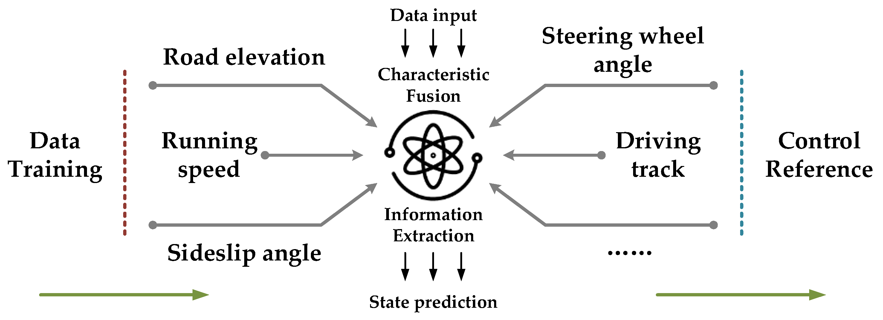
In this paper, the data with variable time-domain length is used as the information input of the LSTM network, and the fusion features of multidimensional data information in different time domains are extracted through dynamic information selection to realize the network offline training based on historical storage information, as shown in Figure 3.
Based on the training results of network features and referring to the real-time information input under the variable length state, the vehicle state of the fused road information can be selected as the current input information and the corresponding features can be extracted to implement and complete the information online prediction under the dynamic data input. Finally, the LSTM network architecture under variable time domain input conditions is completed as shown in Figure 4, and the network state input length in the figure is corrected in real time with the error correction result.
In the prediction process, the length of the data state is optimized according to the real-time calculation error. The calculation process is shown in Section 3.2 below. According to the real-time dynamic prediction results, the system state variable prediction results under the confidence interval can be obtained.

3.2. Optimization Calculation of Variable Time Domain State Length

In the actual offline data training process, the network input should not only consider the impact of historical data on current data, but also prevent excessive historical data from being obliterated and eliminate the impact of current data. Therefore, the network input data length needs to be dynamically adjusted in real time [36]. The operation cycle of the controller is Tc, and the actual output of the network training is Yc = {yc1, yc2,…, yca}. The length of the input data sequence at moment k is Tk, and the corresponding output of network training is Yk = {yk1, yk2, …, ykb}. The corresponding length of the longest data sequence is Tm, and the network training output is Ym = {ym1, ym2, …, ymc}. Considering the storage of historical data, the sequence length of the actual output data of the network is greater than Tk and Tm.
In order to give consideration to data accuracy and calculation speed, according to the actual data sequence dimensions and network output, the reference indicators in the calculation process are defined as:
Δ T = T k     min T c , T m max T c , T m     min T c , T m Δ y = Δ y ¯ k     min Δ y ¯ k , Δ y ¯ m max Δ y ¯ k , Δ y ¯ m     min Δ y ¯ k , Δ y ¯ m
where there are:
Δ y ¯ k = 1 b k j = 1 b k i = 1 b x k i j x c i j 2 b Δ y ¯ m = 1 c m h = 1 c m i = 1 b x m i h x c i h 2 c
where bk and cm are the output times of the network under Tk and Tm data sequence lengths, respectively.
Setting the tolerance range [ε, ζ] under the allowable accuracy requirements of the system, and the objective constraint function is defined as:
F y , T k = min λ 1 Δ T + λ 2 Δ y     ε , ζ
where λ1 and λ2 are the weight coefficients corresponding to ∆T and ∆y, respectively.
Considering the initial sequence length T0, and randomly generating a new length value T* within the range of (0, Tm), where dT = F(y, T0) − F(y, T*). If dT < 0, then Tk = T*, otherwise, Tk = T0. At this time, it is necessary to solve the probability value corresponding to the new value T*, and the corresponding calculation formula is:
P T = e F y , T 0     F y , T T k
The preset number of iterations is D. If the calculated final value T ^ satisfies the objective constraint function, then it is the dynamic optimal data sequence length value, otherwise, the convergence coefficient χ is introduced, and let Tk = χ T ^ . At this time, Tk satisfies the constraint of the objective constraint function, and Tk is defined as the length value of the suboptimal data sequence. The system prediction architecture under a variable time domain input state is shown in Figure 5. After offline training of historical data, the sideslip angle of the centroid obtained through online prediction is input to the controller as the reference for pre-control.

4. Robust Controller Design for Vehicle Stability

The electronic control unit needs to send control commands according to the real-time information input to complete the active decision-making and safety control process of the vehicle during the driving process. The predicted sideslip angle of the centroid is used as the information input and reference to adjust the vehicle stability under dynamic conditions in real time.

4.1. Design of Active Stable Steering Controller

Given the design requirements of vehicle handling and stability controller, and taking into account the model accuracy, numerical calculation ability and algorithm applicability, it is assumed that the steering angles of wheels on both sides of the coaxial line are the same during the design process. The simplified vehicle system steering dynamics model can be obtained as shown in Figure 6 [37].
In this model, the wheel angles on both sides of the vehicle axis are the same, so the four-wheel steering control of the vehicle can be transformed into the active control of the front and rear wheels. The front and rear axle track widths of the vehicle are approximately equal, and the lateral distance between the left and right wheels and the centroid is also approximately equal. During driving, the tire always keeps in contact with the ground.
Based on the above assumptions, the simplified vehicle dynamics equation can be obtained as follows:
m a y = F y f cos δ f + F y r cos δ r I z ω ˙ L f F y f sin δ f L r F y r sin δ r a y = v ˙ y + v x ω v x β ˙ + ω
As for four-wheel steering vehicles, the front and rear tire sideslip angles can be obtained as follows:
α f = β + L f ω v x δ f α r = β L r ω v x δ r
In the actual high-speed driving process, the steering angle of the vehicle is small, so the equivalent lateral dynamic equation of the vehicle system can be obtained as [38]:
m v x β ˙ + ω K f β + L f ω v x δ f K r β L r ω v x δ r I z ω ˙ L f K f β + L f ω v x δ f + L r K r β L r ω v x δ r
By further transforming the above equation, the system equation can be obtained as follows:
β ˙ = K f   +   K r m v x β L f K f     L r K r m v x 2 + 1 ω + K f δ f   +   K r δ r m v x ω ˙ = L f K f     L r K r I z β L f 2 K f   +   L r 2 K r I z v x ω + L f K f δ f     L r K r δ r I z
The system state equation becomes the following form:
x ˙ = A x + B u β ˙ ω ˙ = A 11 A 12 A 21 A 22 β ω + B 11 B 12 B 21 B 22 δ f δ r
where there are:
A 11 = K f + K r m v x ,   A 12 = L f K f L r K r m v x 2 + 1 ,   A 21 = L f K f L r K r I z ,   A 22 = L f 2 K f + L r 2 K r I z v x
B 11 = K f m v x , B 12 = K r m v x , B 21 = L f K f I z , B 22 = L r K r I z
Considering the influence of correlation coefficient cev between front wheel angle and rear wheel angle, there is the following corresponding relationship:
δ r = c e δ f
Further, consider the correlation between the rear wheel angle and the front wheel angle, so the above Formula (26) can be substituted into the vehicle dynamics model to obtain the response of the vehicle front wheel angle δf. On this basis, the Laplace transform is carried out and the steady value of the centroid sideslip angle β can be calculated, then the following derivation results are obtained:
β s δ f s = K f + c e K r m v x + L f K f L r K r v x L f K f c e L r K r L f 2 K f + L r 2 K r v x m v x s + K f + K r m v x + L f K f L r K r v x L f K f L r K r L f 2 K f + L r 2 K r v x
When the centroid sideslip angle β is 0, the following results can be obtained by solving the correlation coefficient ce:
c e = m v x 2 L f K f L K f L r K r m v x 2 L r K r + L L f K f K r = m v x 2 L f L K r L r m v x 2 L r K f L + L f = L r m v x 2 L f L L r K r 1 L f m v x 2 L r L L f K f + 1
Based on the above correlation, the system equation is transformed into:
x ˙ = A x + B u β ˙ ω ˙ = A 11 A 12 A 21 A 22 β ω + B 1 B 2 δ f
where
B 1 = K f + c e K r m v x ,   B 2 = L f K f c e L r K r I z
Through further derivation, it is obtained that the transfer function of the front wheel angle δf relative to the sideslip angle of the centroid β is as:
G s = B 1 s + A 12 B 2 A 22 B 1 s 2 A 11 A 22 s + A 11 A 22 A 12 A 12
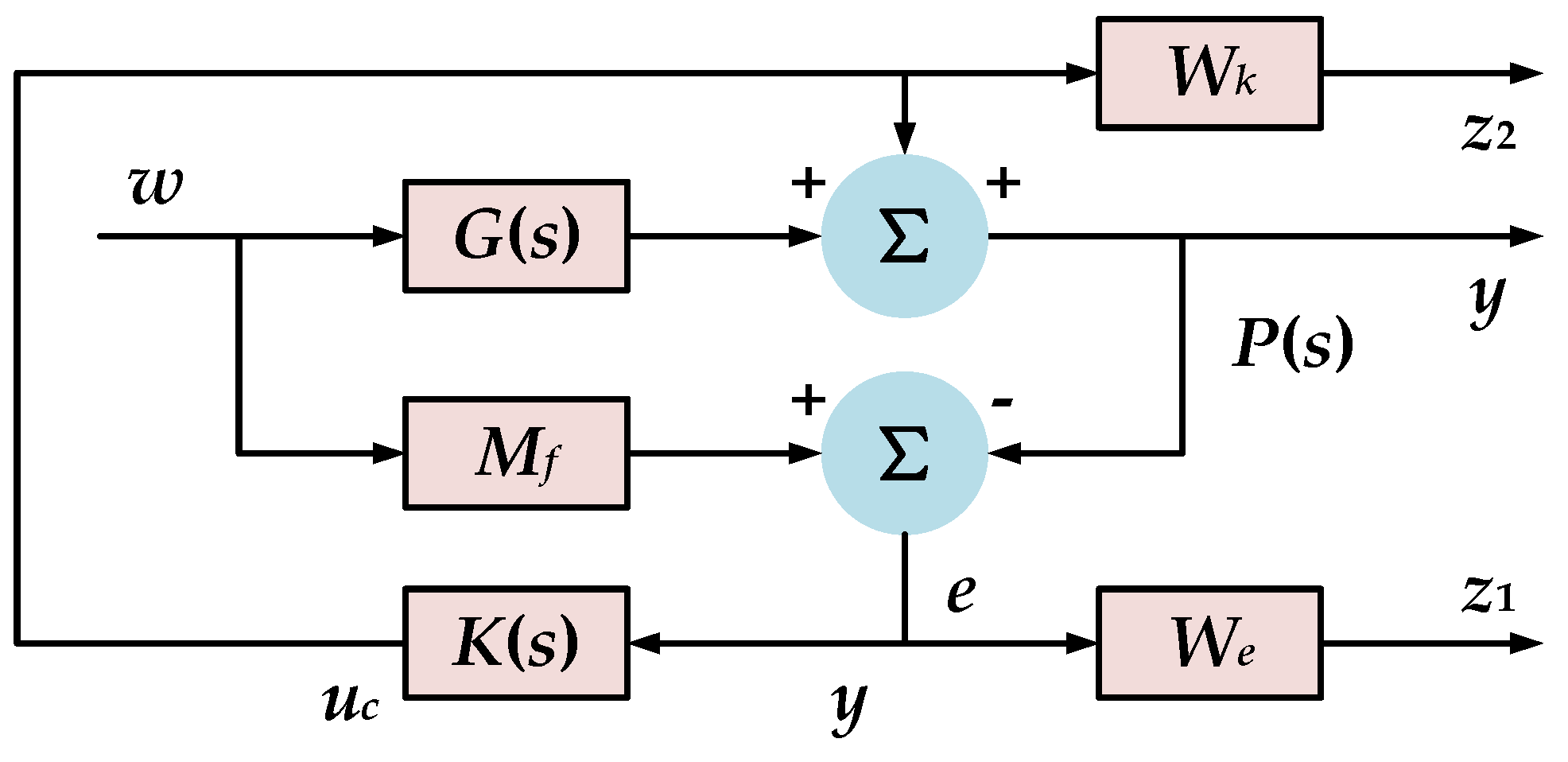
The principle of the sideslip angle closed-loop system control model of the four-wheel steering system studied is shown in Figure 7. In Figure 7, Mf is the reference model of the centroid sideslip angle, yo is the system signal feedback, and uc is the system control input. The weight value parameters We and Wk are introduced, and the system output matrix can be obtained as follows:
z y = z 1 z 2 y = W e M f G 0 0 W k M f G 0 δ f u c

4.2. Solution of Mixed Sensitivity Problem of System

Assuming that the control model and real system model correspond to G(s) and Gr(s), respectively, and the system transfer function is Mt(s). The model uncertainty function induced by the difference between the two models is Ξ(s) and the optimal controller of the system corresponds to K(s). Then, when the uncertainty function Ξ(s) is stable, the bounded input of the system corresponds to the bounded output, and the following transfer relationship is obtained:
M t j ω Ξ j ω < 1 ,   ω         M t j ω M u j ω < 1 ,   ω
where Mu() is the supremum corresponding to the uncertainty function Ξ(s).
The limit optimization of a single performance will cause an imbalance in the overall performance of the system. In order to avoid the above problem, it is necessary to consider the interaction and influence of system multi-performance in the design process of the optimal controller. Therefore, the controller design needs to consider the multi-performance evaluation system and system compatibility and realizes the system-integrated control optimization process under multi objectives, which depends on the solution of the following mixed sensitivity [39].
According to this premise, the system output transfer function is:
z = G A 11 + G A 12 I G A 22 K 1 G A 21 Γ = G G A , K Γ G A = G A 11 G A 12 G A 21 G A 22 = I 0 I G I G T = W e M f G 0 M f G 0 W k 0 T
where Γ denotes the external signal matrix and GA denotes the system model augmented matrix.
The system sensitivity problem is converted into the following solution problem:
min K   stabilising J = I + G K 1 K I + G K 1 min K   stabilising J = W e I + G K 1 W k K I + G K 1
In order to facilitate the practical engineering application, the optimal solution of the controller in the calculation process is converted into the suboptimal solution of the stability controller K(s), which makes the H norm of the closed-loop transfer function less than a positive value κ. At this time, the transfer function satisfies the following constraint condition:
min G G A , K < κ
within the allowable error range, the linear matrix inequality (LMI) method can be employed to solve the above optimization control problems so that the parameter optimization controller K(s) can be calculated [40].
Based on this, the target values δtf and δtr of the front wheel angle and rear wheel angle of the vehicle can be obtained successively. According to the error value between the corresponding actual angles δf, δr and the target angles δtf, δtr, it can be calculated that the motor drive current idf and idr under the driving process of front and rear wheel active steering are respectively as:
i d f = i p f e δ f t + i i f e δ f t d t + i d f d e δ f t d t ,   e δ f t = δ t f t δ f t i d r = i p r e δ r t + i i r e δ r t d t + i d r d e δ r t d t ,   e δ r t = δ t r t δ r t
where, ipf, ipr, iif, iir, idf, and idr are the proportional, integral, and differential coefficients under the control of the front and rear wheel proportion integration differentiation (PID) controllers of the vehicle, respectively.

5. Discussion on Research Results of System Numerical Calculation

In order to validate the robustness and effectiveness of the system steering control strategy under external disturbance and excitation, different working conditions of road elevation information varying with driving mileage are constructed to fully verify the system stability control effect under non-ideal road conditions. At the same time, the influence of external stochastic excitation on the steering system also needs to be fully considered.
According to the coupling relationship between the vehicle dynamics model, state prediction network architecture, and mixed sensitivity controller, numerical simulation can be carried out for different working conditions. In the actual numerical solution process, the time step is set to 0.001 s, and the following simulation conditions were set to study and verify the stability of the vehicle.

5.1. Numerical Calculation Research under Condition 1

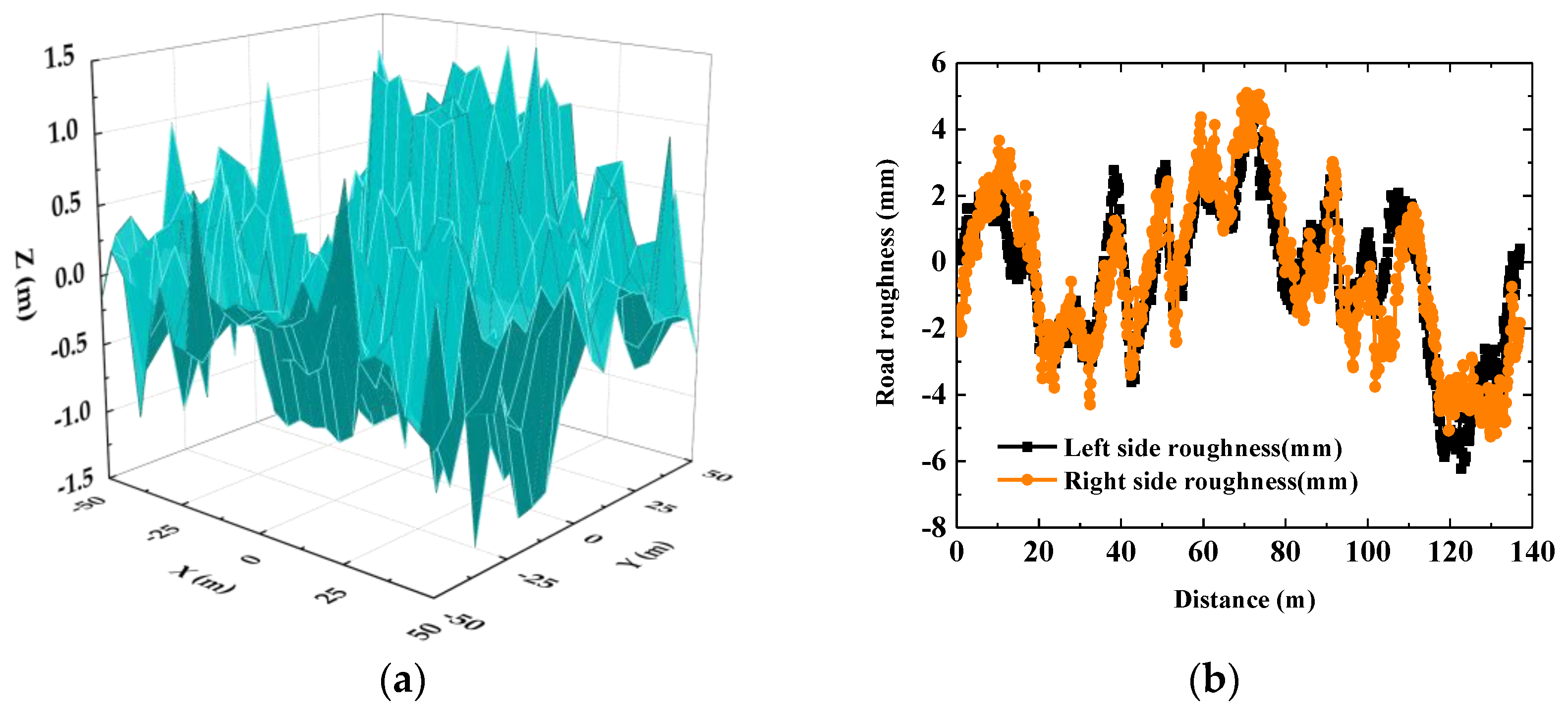
The vehicle traveled on the cross-country mountain road at the speed of 24 km/h, and the road adhesion coefficient μ = 0.75. The relationship between the change of road vertical height and the change of horizontal and vertical coordinate positions is shown in Figure 8a. In addition, the change of road roughness on the ground of the left and right wheels of the vehicle at the specific location is shown in Figure 8b. The difference between Figure 8a and Figure 8b is the coupling condition setting of road elevation information and external road excitation. The proposed control strategy is verified by the superposition of multi-source excitation in the time domain.
According to the corresponding numerical calculation results of condition 1, the corresponding system dynamic response results can be obtained as shown in Figure 9a–d. Under off-road conditions, the vehicle driving path is coupled with road roughness. Under the condition of coupling information input, the vehicle performs open-loop control in an off-road environment. At this time, there is no target track tracking feedback information, and the controller realizes the vehicle system stability control through the active steering control of four wheels.
As shown in Figure 9a, during the open-loop control process, the vehicle system without control tends to be unstable. With the extension of the calculation time scale, compared with the system state response under control, the vehicle trajectory under no control tended to be unstable, and the corresponding root mean square (RMS) value of the lateral acceleration is 0.61 g. The sideslip angle of the centroid repeatedly oscillated between 12° and 25°, and the lateral acceleration fluctuated in a large range. With the extension of the driving distance, the amplitude of its oscillation became increasingly larger, which indicates that the system at this time was unstable. Further analysis of the system states under control shows that the driving track of vehicles without state predictor is close to that of vehicles with state predictor, and the corresponding RMS values of the lateral acceleration were 0.56 g and 0.55 g, respectively, which were less than the lateral acceleration under no control. At the same time, the RMS values of the sideslip angle and yaw rate at the centroid corresponding to different control modes are shown in Table 2. From the data in Table 2, it can be intuitively seen that the system state under predictive control is better than that under no control.
Although according to the data results in Table 2, whether the predictive controller exists or not, its corresponding root mean square value of vehicle state is relatively close. However, it can be intuitively seen from Figure 9c that under the input of prediction information, the vehicle state recovers to the stable region faster, which is particularly important for vehicle stability control under complex coupled working conditions.

5.2. Numerical Calculation Research under Condition 2

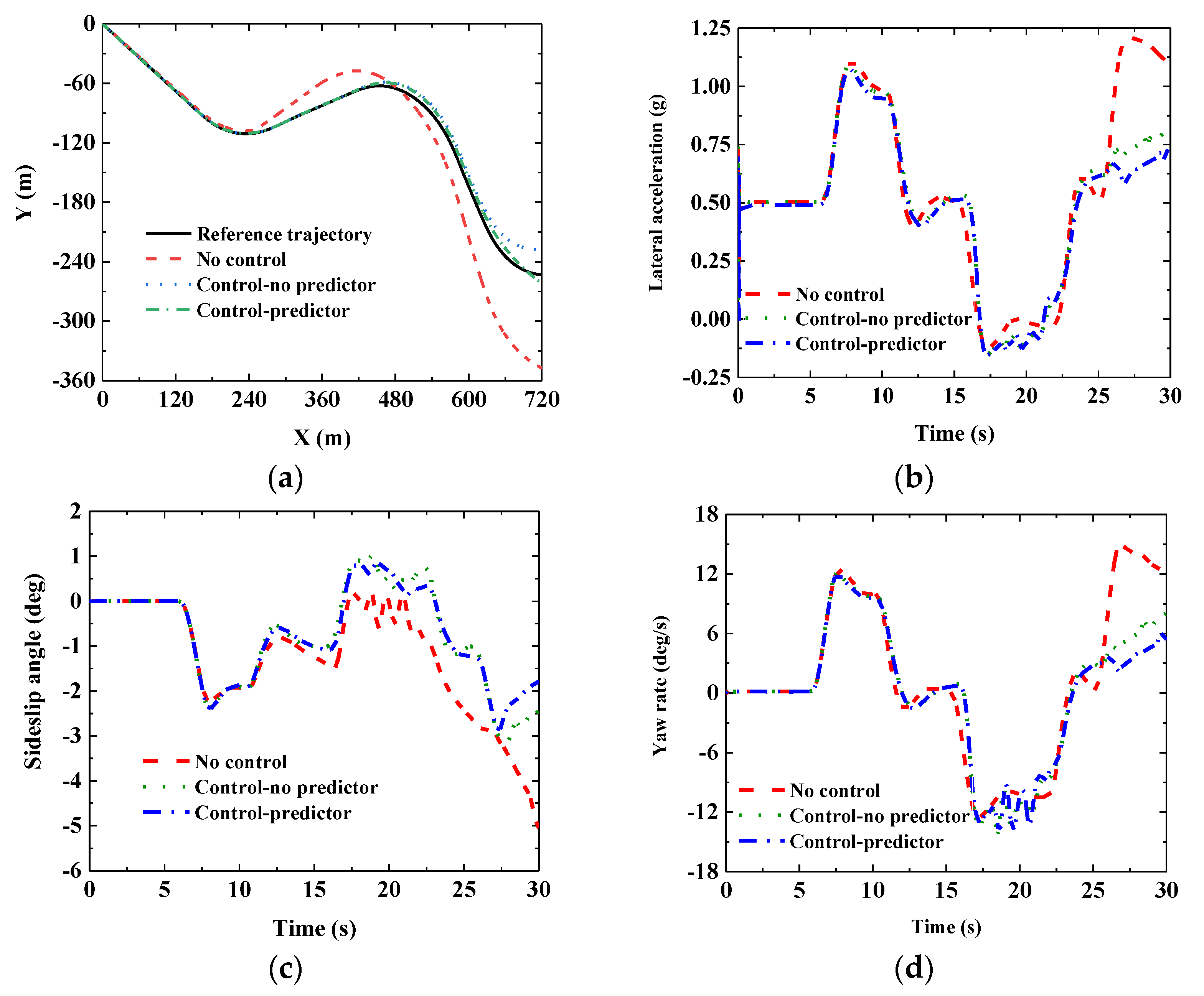
At this time, the relationship between the vertical height of the road and the horizontal and vertical coordinate positions is shown in Figure 10. At the same time, the vehicle traveled along the target road track as shown in Figure 11a, the driving speed was set to 100 km/h, and the road adhesion coefficient μ = 0.85.
According to the setting of condition 2, the vehicle implemented system closed-loop control along the predetermined road, and the system dynamic response results can be obtained through numerical calculation, as shown in Figure 11a–d.
According to the simulation results, during the high-speed traveling along the target track, the vehicle without control gradually lost its stability and deviated from the normal track. The RMS of the corresponding lateral acceleration of the unstable vehicle was 0.68 g, and the RMS value of the yaw rate was 8.01°. The sideslip angle of the centroid gradually deviated from the normal value, and the final error cannot converge. The vehicle under control could keep stable, and its corresponding RMS values of vehicle state are shown in Table 3, and its driving track could move along the target track. However, it can be seen from the actual driving path that the vehicle with state prediction as the reference input could better travel along the target track, and its actual control effect was more accurate. If time continues to stretch, it can be seen from the driving track in Figure 11a that the vehicle driving track under stateless prediction will gradually deviate, and the resulting error will gradually increase. In addition, by further comparing the RMS values corresponding to the three state quantities in Table 3, it can be seen that the system control effect under the action of the predictive network is more prominent, so real-time state prediction in the stability control process is necessary.
Although the state data of the vehicle system with or without the predictive controller in Table 3 are similar, it can be seen from the data change curve in Figure 11c,d that the vehicle system with the predictive controller can keep the vehicle stable in a safe area. Moreover, because of the input of predictive data, the system state can quickly return to the safe area, which is critical to the safety and stability of vehicles during driving. Table 2 and Table 3 only further quantify the effect of control, but the actual control effect must be reflected according to the response curve in Figure 9 and Figure 11.

6. Conclusions

In the process of multi-dimensional data interaction and fusion, in order to achieve accurate vehicle stability control, control strategies can be formulated in advance during real-time prediction data interaction through existing information feature extraction to complete information preview and system stability control based on current vehicle states.
In order to realize real-time calculation and state prediction based on historical information and solve the vehicle stability control problem in the actual driving process, this paper builds a system nonlinear dynamic model for four-wheel steering vehicles. On this basis, the LSTM network calculation model with variable time domain information input was constructed based on error feedback by making full use of the vehicle historical data under multiple working conditions so that the online prediction of vehicle status is realized based on variable scale time domain information. This was taken as the reference input of the controller, and then the vehicle stability robust controller with zero sideslip angle was designed according to the monorail vehicle model to solve the numerical solution process of the system model under the mixed sensitivity problem of the system. The numerical results under different working conditions show that compared with the system without control, the vehicle under the action of a robust controller has higher safety and stability. At the same time, the controller input under the system information prediction can achieve higher control accuracy, which is of great significance for the active safety control of vehicles and the active intervention of drivers.

Author Contributions

This research was jointly completed by all authors, and the specific work assignments are as follows: the original research idea was jointly revised and completed by Z.G., J.F. and C.W.; The implementation method was jointly discussed and completed by Z.G., Y.C., T.Z. and B.Q.; S.T. and T.M. jointly verified the research results; Z.G., B.Q. and T.Z. jointly completed the software compilation and debugging; Y.H. and J.X. summarized and improved the literature review. All authors jointly completed the writing, discussion, and revision of the manuscript. All authors have read and agreed to the published version of the manuscript.

Funding

This research was supported by the National Natural Science Foundation of China under Grant 52002025, the National Natural Science Foundation of China under Grant 52102445, and the Subsidy for Young Teachers’ Scientific Research Ability Improvement Program under grant X21050.

Informed Consent Statement

Informed consent was obtained from all subjects involved in the study.

Conflicts of Interest

The authors declare no conflict of interest.

References

  1. Song, X.; Li, X.; Tang, W.; Zhang, W. A fusion strategy for reliable vehicle positioning utilizing RFID and in-vehicle sensors. Inf. Fusion 2016, 31, 76–86. [Google Scholar] [CrossRef]
  2. Zhang, L.; Zhang, Z.Q.; Wang, X.P.; Deng, J.J.; Dorrell, D.G. Chassis Coordinated Control for Full X-by-Wire Vehicles-A Re-view. Chin. J. Mech. Eng. 2021, 34, 42. [Google Scholar] [CrossRef]
  3. Rajput, S.K.; Patni, J.C.; Alshamrani, S.S.; Chaudhari, V.; Dumka, A.; Singh, R.; Rashid, M.; Gehlot, A.; AlGhamdi, A.S. Au-tomatic Vehicle Identification and Classification Model Using the YOLOv3 Algorithm for a Toll Management System. Sustainability 2022, 14, 9163. [Google Scholar] [CrossRef]
  4. Dong, J.; Zhuang, D.; Huang, Y.; Fu, J. Advances in Multi-Sensor Data Fusion: Algorithms and Applications. Sensors 2009, 9, 7771–7784. [Google Scholar] [CrossRef] [PubMed] [Green Version]
  5. Kang, M.; Lee, W.; Hwang, K.; Yoon, Y. Vision Transformer for Detecting Critical Situations and Extracting Functional Scenario for Automated Vehicle Safety Assessment. Sustainability 2022, 14, 9680. [Google Scholar] [CrossRef]
  6. Yao, X.; Gu, X.; Jiang, P. Coordination control of active front steering and direct yaw moment control based on stability judgment for AVs stability enhancement. Proc. Inst. Mech. Eng. Part D: J. Automob. Eng. 2021, 236, 59–74. [Google Scholar] [CrossRef]
  7. Kim, B.; Yi, K. Probabilistic and Holistic Prediction of Vehicle States Using Sensor Fusion for Application to Integrated Vehicle Safety Systems. IEEE Trans. Intell. Transp. Syst. 2014, 15, 2178–2190. [Google Scholar] [CrossRef]
  8. Mozaffari, S.; Al-Jarrah, O.Y.; Dianati, M.; Jennings, P.; Mouzakitis, A. Deep Learning-Based Vehicle Behavior Prediction for Autonomous Driving Applications: A Review. IEEE Trans. Intell. Transp. Syst. 2020, 23, 33–47. [Google Scholar] [CrossRef]
  9. Hsu, L.-Y.; Chen, T.-L. Vehicle Full-State Estimation and Prediction System Using State Observers. IEEE Trans. Veh. Technol. 2008, 58, 2651–2662. [Google Scholar] [CrossRef]
  10. Qian, L.P.; Feng, A.; Yu, N.; Xu, W.; Wu, Y. Vehicular Networking-Enabled Vehicle State Prediction via Two-Level Quantized Adaptive Kalman Filtering. IEEE Internet Things J. 2020, 7, 7181–7193. [Google Scholar] [CrossRef]
  11. Xing, Y.; Lv, C.; Cao, D.; Lu, C. Energy oriented driving behavior analysis and personalized prediction of vehicle states with joint time series modeling. Appl. Energy 2020, 261, 114471. [Google Scholar] [CrossRef]
  12. Jo, Y.; Jang, J.; Ko, J.; Oh, C. An In-Vehicle Warning Information Provision Strategy for V2V-Based Proactive Traffic Safety Management. IEEE Trans. Intell. Transp. Syst. 2022, 23, 19387–19398. [Google Scholar] [CrossRef]
  13. Xiao, H.P.; Wang, C.Q.; Li, Z.X.; Wang, R.D.; Bo, C.; Sotelo, M.A.; Xu, Y.c. UB-LSTM: A Trajectory Prediction Method Com-bined with Vehicle Behavior Recognition. J. Adv. Trans. 2021, 2020, 8859689. [Google Scholar]
  14. Shi, K.; Yuan, X.; He, Q. Double-layer Dynamic Decoupling Control System for the Yaw Stability of Four Wheel Steering Vehicle. Int. J. Control. Autom. Syst. 2019, 17, 1255–1263. [Google Scholar] [CrossRef]
  15. Lee, S.-H.; Lee, U.-K.; Ha, S.-K.; Han, C.-S. Four-Wheel Independent Steering (4WIS) System for Vehicle Handling Improvement by Active Rear Toe Control. JSME Int. J. Ser. C 1999, 42, 947–956. [Google Scholar] [CrossRef] [Green Version]
  16. Riccardo, M.; Stefano, S.; Fabio, C. Nonlinear PI front and rear steering control in four wheel steering vehicles. Veh. Syst. Dyn. 2007, 45, 1149–1168. [Google Scholar]
  17. Marino, R.; Cinili, F. Input–Output Decoupling Control by Measurement Feedback in Four-Wheel-Steering Vehicles. IEEE Trans. Control Syst. Technol. 2009, 17, 1163–1172. [Google Scholar] [CrossRef]
  18. Tian, J.; Ding, J.; Tai, Y.; Chen, N. Hierarchical Control of Nonlinear Active Four-Wheel-Steering Vehicles. Energies 2018, 11, 2930. [Google Scholar] [CrossRef] [Green Version]
  19. Meng, Q.; Sun, Z.-Y.; Li, Y. Finite-time Controller Design for Four-wheel-steering of Electric Vehicle Driven by Four In-wheel Motors. Int. J. Control Autom. Syst. 2018, 16, 1814–1823. [Google Scholar] [CrossRef]
  20. Wang, C.; Heng, B.; Zhao, W. Yaw and lateral stability control for four-wheel-independent steering and four-wheel-independent driving electric vehicle. Proc. Inst. Mech. Eng. Part D J. Automob. Eng. 2019, 234, 409–422. [Google Scholar] [CrossRef]
  21. He, S.; Tang, T.; Ye, M.; Xu, E.; Deng, J.; Tang, R. A domain association hierarchical decomposition optimization method for cab vibration control of commercial vehicles. Measurement 2019, 138, 497–513. [Google Scholar] [CrossRef]
  22. He, S.; Tang, T.; Xu, E.; Ye, M.; Zheng, W. Vibration control analysis of vehicle steering system based on combination of finite-element analysis and modal testing. J. Vib. Control 2019, 26, 88–101. [Google Scholar] [CrossRef]
  23. Yang, L.; Luo, J.C.; Song, X.W.; Li, M.L.; Wen, P.W.; Xiong, Z.X. Robust Vehicle Speed Measurement Based on Feature In-formation Fusion for Vehicle Multi-Characteristic Detection. Entropy 2021, 23, 910. [Google Scholar] [CrossRef] [PubMed]
  24. Mazzilli, V.; De Pinto, S.; Pascali, L.; Contrino, M.; Bottiglione, F.; Mantriota, G.; Gruber, P.; Sorniotti, A. Integrated chassis control: Classification, analysis and future trends. Annu. Rev. Control 2021, 51, 172–205. [Google Scholar] [CrossRef]
  25. Im, S.J.; Oh, J.S.; Kim, G.-W. Simultaneous Estimation of Unknown Road Roughness Input and Tire Normal Forces Based on a Long Short-Term Memory Model. IEEE Access 2022, 10, 16655–16669. [Google Scholar] [CrossRef]
  26. Hang, P.; Chen, X. Towards Autonomous Driving: Review and Perspectives on Configuration and Control of Four-Wheel Independent Drive/Steering Electric Vehicles. Actuators 2021, 10, 184. [Google Scholar] [CrossRef]
  27. Kim, J. Effect of vehicle model on the estimation of lateral vehicle dynamics. Int. J. Automot. Technol. 2010, 11, 331–337. [Google Scholar] [CrossRef]
  28. Dahmani, H.; Pages, O.; El Hajjaji, A.; Daraoui, N. Observer-Based Robust Control of Vehicle Dynamics for Rollover Mitigation in Critical Situations. IEEE Trans. Intell. Transp. Syst. 2013, 15, 274–284. [Google Scholar] [CrossRef]
  29. Zhao, W.Z.; Li, Y.J.; Wang, C.Y.; Zhang, Z.Q.; Xu, C.L. Research on control strategy for differential steering system based on H mixed sensitivity. Int. J. Automot. Technol. 2013, 14, 913–919. [Google Scholar] [CrossRef]
  30. Yu, Y.; Si, X.; Hu, C.; Zhang, J. A Review of Recurrent Neural Networks: LSTM Cells and Network Architectures. Neural Comput. 2019, 31, 1235–1270. [Google Scholar] [CrossRef]
  31. Graber, T.; Lupberger, S.; Unterreiner, M.; Schramm, D. A Hybrid Approach to Side-Slip Angle Estimation With Recurrent Neural Networks and Kinematic Vehicle Models. IEEE Trans. Intell. Veh. 2018, 4, 39–47. [Google Scholar] [CrossRef]
  32. Wang, J.; Li, X.; Li, J.; Sun, Q.; Wang, H. NGCU: A New RNN Model for Time-Series Data Prediction. Big Data Res. 2021, 27, 100296. [Google Scholar] [CrossRef]
  33. Zhu, J.; Sun, K.; Jia, S.; Lin, W.; Hou, X.; Liu, B.; Qiu, G. Bidirectional Long Short-Term Memory Network for Vehicle Behavior Recognition. Remote Sens. 2018, 10, 887. [Google Scholar] [CrossRef] [Green Version]
  34. Shi, Y.; Li, Y.; Fan, J.; Wang, T.; Yin, T. A Novel Network Architecture of Decision-Making for Self-Driving Vehicles Based on Long Short-Term Memory and Grasshopper Optimization Algorithm. IEEE Access 2020, 8, 155429–155440. [Google Scholar] [CrossRef]
  35. Yeon, K.; Min, K.; Shin, J.; Sunwoo, M.; Han, M. Ego-Vehicle Speed Prediction Using a Long Short-Term Memory Based Re-current Neural Network. Int. J. Automot. Technol. 2019, 20, 713–722. [Google Scholar] [CrossRef]
  36. Hao, W.; Rong, D.; Yi, K.; Zeng, Q.; Gao, Z.; Wu, W.; Wei, C.; Scepanovic, B. Traffic Status Prediction of Arterial Roads Based on the Deep Recurrent Q-Learning. J. Adv. Transp. 2020, 2020, 1–17. [Google Scholar] [CrossRef]
  37. Wang, J.; Wang, R.; Jing, H.; Chen, N. Coordinated Active Steering and Four-Wheel Independently Driving/Braking Control with Control Allocation. Asian J. Control 2015, 18, 98–111. [Google Scholar] [CrossRef]
  38. Wu, Y.; Wang, L.F.; Zhang, J.Z.; Li, F. Robust vehicle yaw stability controlby active front steering with active disturbance rejection controller. Proc. Inst. Mech. Eng. Part I J. Syst. Control Eng. 2019, 233, 1127–1135. [Google Scholar] [CrossRef]
  39. Zhu, S.; Gelbal, S.Y.; Aksun-Guvenc, B.; Guvenc, L. Parameter-Space Based Robust Gain-Scheduling Design of Automated Vehicle Lateral Control. IEEE Trans. Veh. Technol. 2019, 68, 9660–9671. [Google Scholar] [CrossRef]
  40. Elmi, N.; Ohadi, A.; Samadi, B. Active front-steering control of a sport utility vehicle using a robust linear quadratic regulator method, with emphasis on the roll dynamics. Proc. Inst. Mech. Eng. Part D J. Automob. Eng. 2013, 227, 1636–1649. [Google Scholar] [CrossRef]
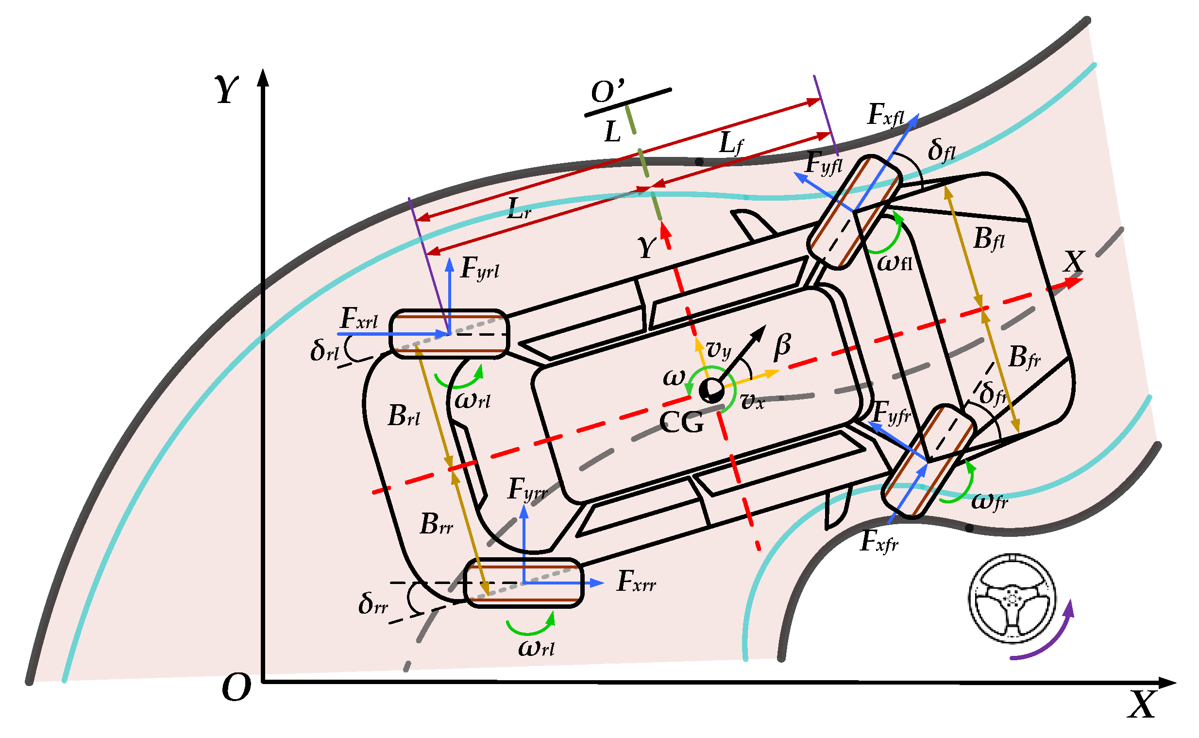
Figure 1. Vehicle system dynamics model.
Sustainability 15 00114 g001
Figure 2. Tire lateral force under variable load.
Sustainability 15 00114 g002
Figure 3. Data fusion and feature extraction.
Sustainability 15 00114 g003
Figure 4. LSTM Structure with variable time domain input.
Sustainability 15 00114 g004
Figure 5. Variable time domain vehicle state prediction architecture.
Sustainability 15 00114 g005
Figure 6. Dynamic model of monorail vehicle.
Sustainability 15 00114 g006
Figure 7. Dynamic control model of monorail vehicle.
Sustainability 15 00114 g007
Figure 8. Road information input: (a) driving road elevation dynamic quantity and (b) roughness of left and right roads.
Sustainability 15 00114 g008
Figure 9. System state responses under condition 1: (a) driving track; (b) lateral acceleration of the centroid; (c) sideslip angle of the centroid; and (d) yaw angular velocity of the centroid.
Sustainability 15 00114 g009
Figure 10. Dynamic variation of road elevation.
Sustainability 15 00114 g010
Figure 11. System state responses under condition 2: (a) driving track; (b) lateral acceleration of the centroid; (c) sideslip angle of the centroid; and (d) yaw angular velocity of the centroid.
Sustainability 15 00114 g011
Table 1. Vehicle states parameter setting.
States ParametersParameter ValueUnit
mb1455kg
m1775kg
Lf1070mm
Lr1560mm
Bi(i = fl, fl, rl, rr)915mm
Ix730.5kg·m2
Iy2260.5kg·m2
Iz2260.5kg·m2
Ad2.9m2
Cd0.3
Table 2. RMS values of system state under working condition 1.
Centroid States ParametersLateral Acceleration (g)Sideslip Angle (deg)Yaw Rate (deg)
No predictive control0.562.9023.90
Predictive control0.552.5620.91
Table 3. RMS values of system state under working condition 2.
Centroid States ParametersLateral Acceleration (g)Sideslip Angle (deg)Yaw Rate (deg)
No predictive control0.601.346.84
Predictive control0.571.206.52
Disclaimer/Publisher’s Note: The statements, opinions and data contained in all publications are solely those of the individual author(s) and contributor(s) and not of MDPI and/or the editor(s). MDPI and/or the editor(s) disclaim responsibility for any injury to people or property resulting from any ideas, methods, instructions or products referred to in the content.