
Analysis of Wave Energy Behavior and Its Underlying Reasons in the Gulf of Mexico Based on Computer Animation and Energy Events Concept


Abstract
:1. Introduction
2. Methods
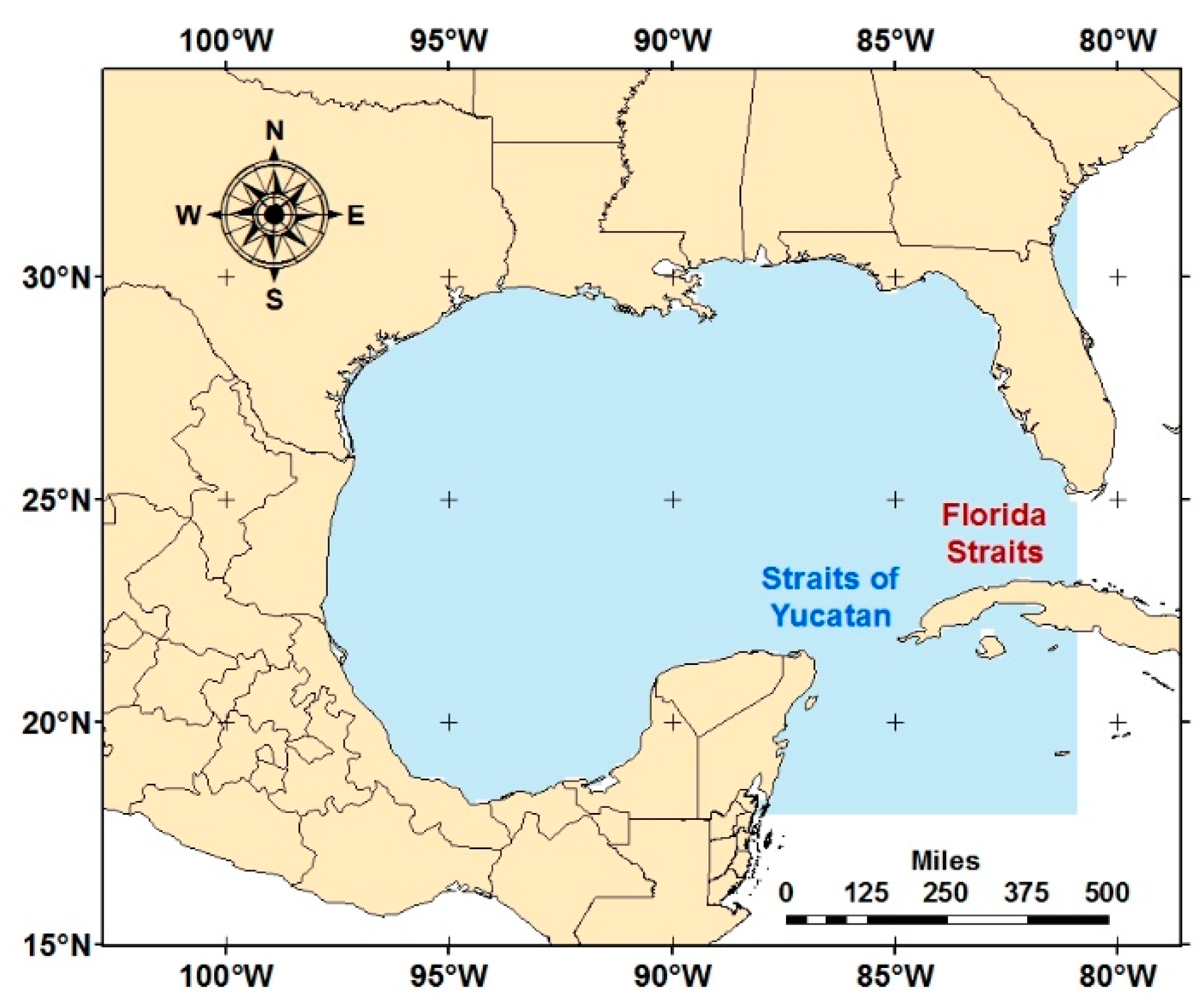
2.1. Meteorological Data and Studying Area
2.2. Limitation of Static Methods
2.3. GIS Big Data Animation with Energy Events
3. Results
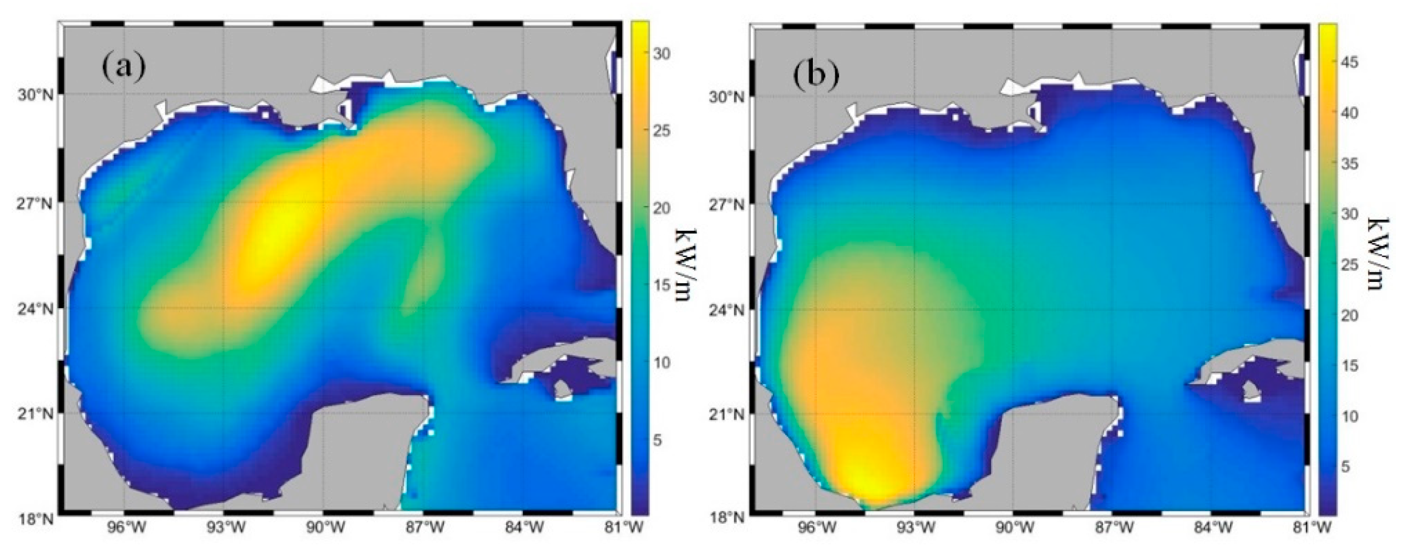
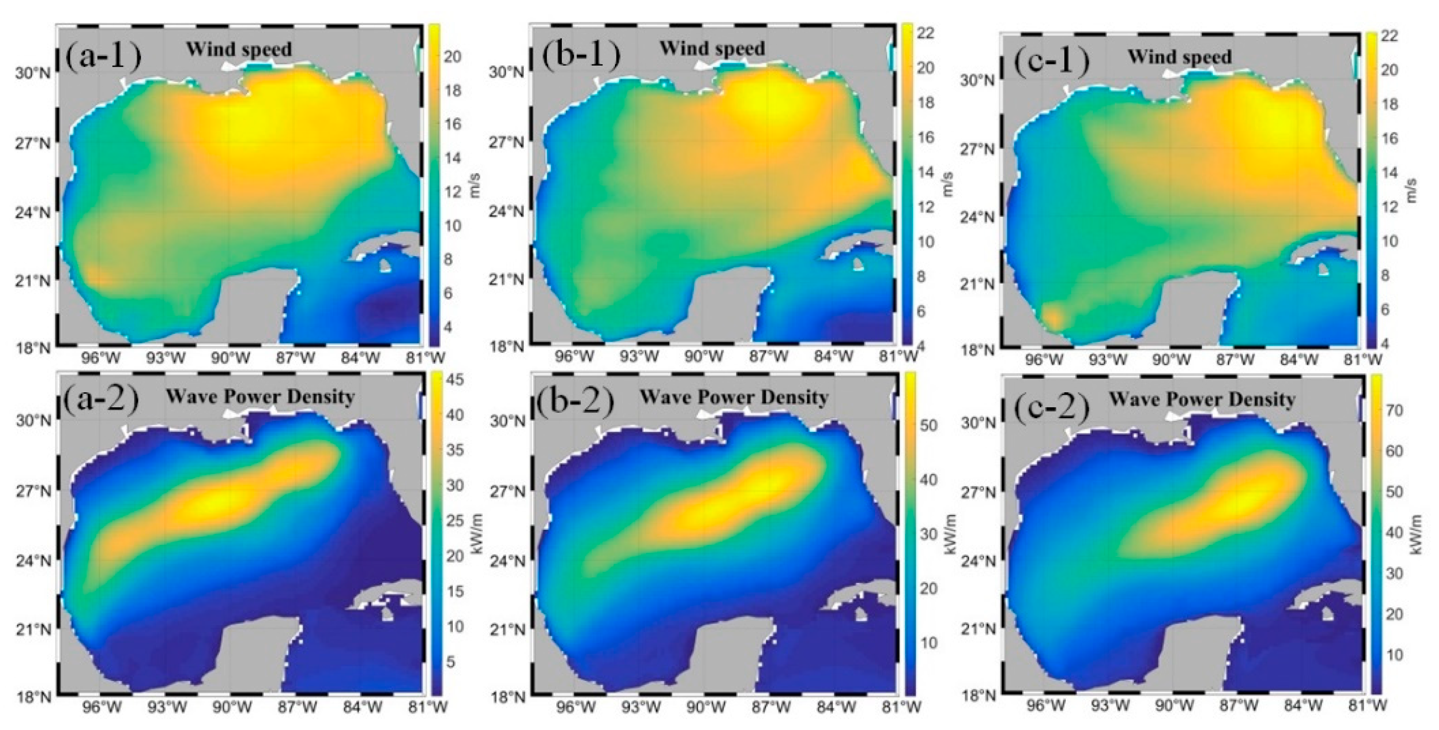
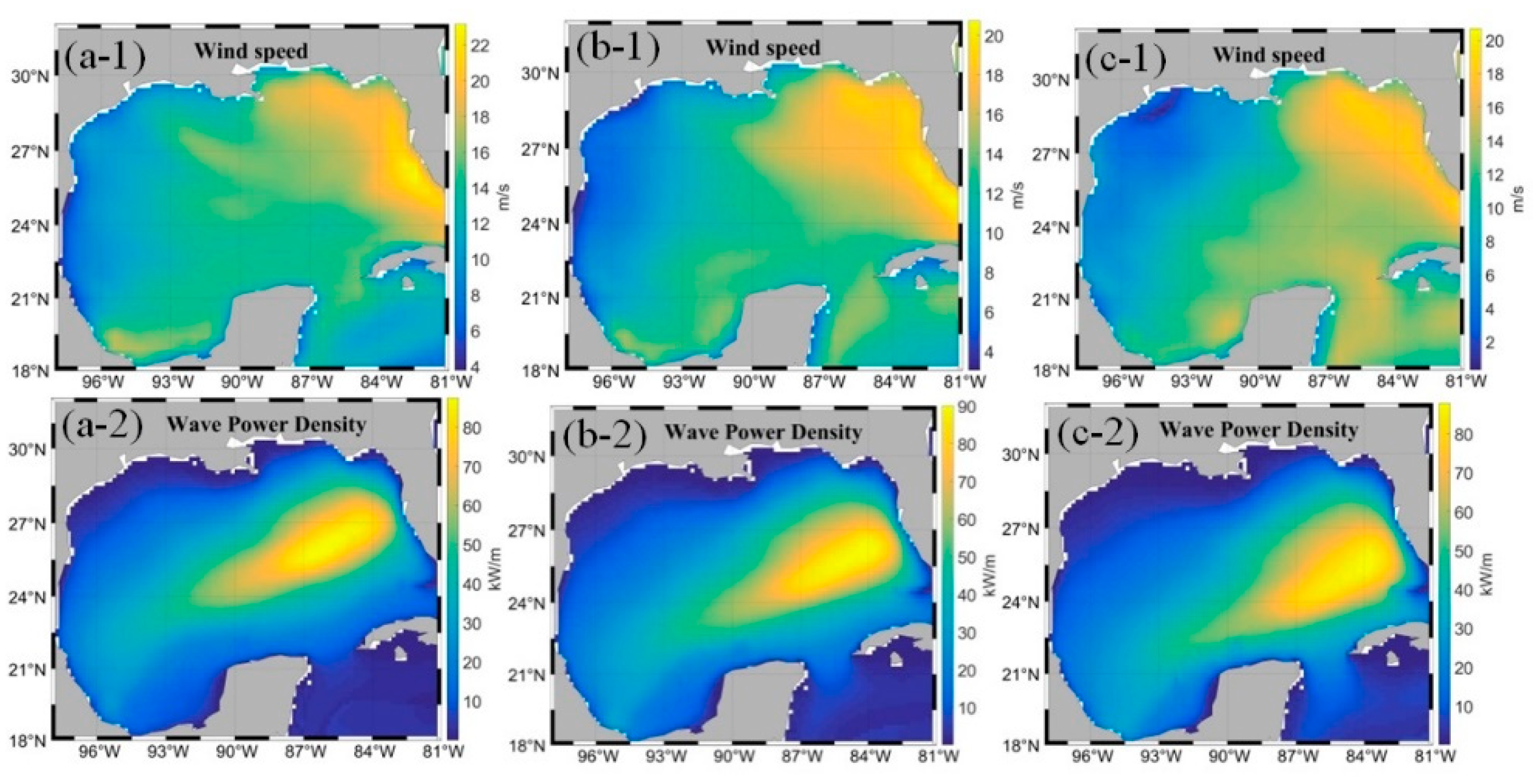
3.1. Qualitative Analysis of High Levels of Wave Energy Behavior in the GoM
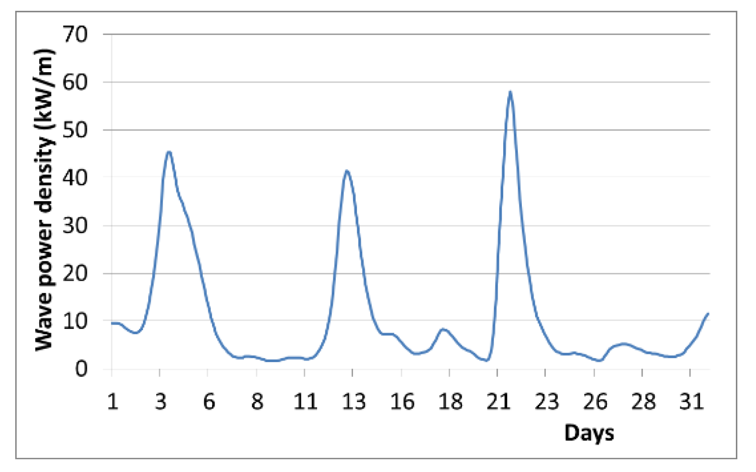
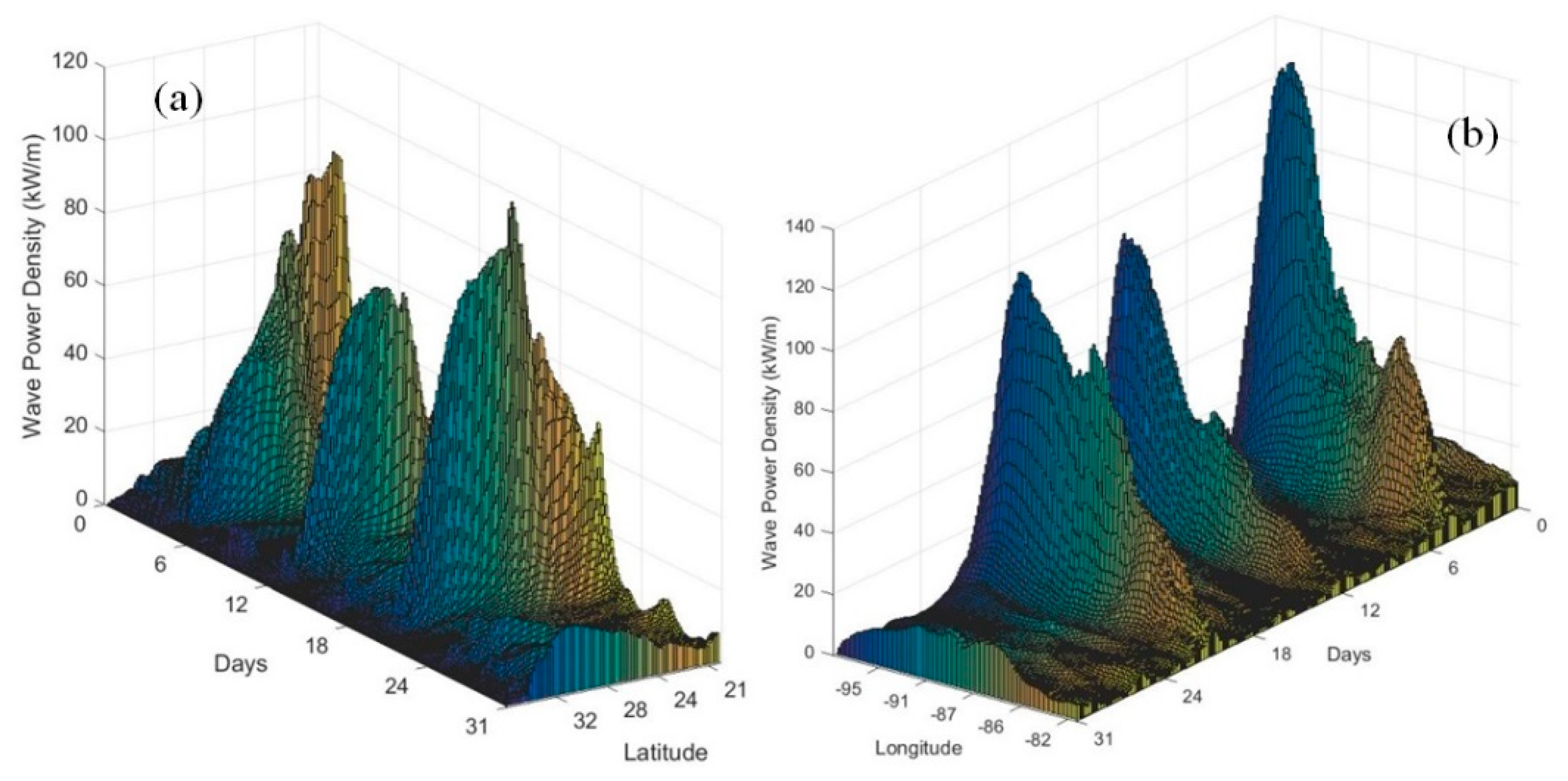
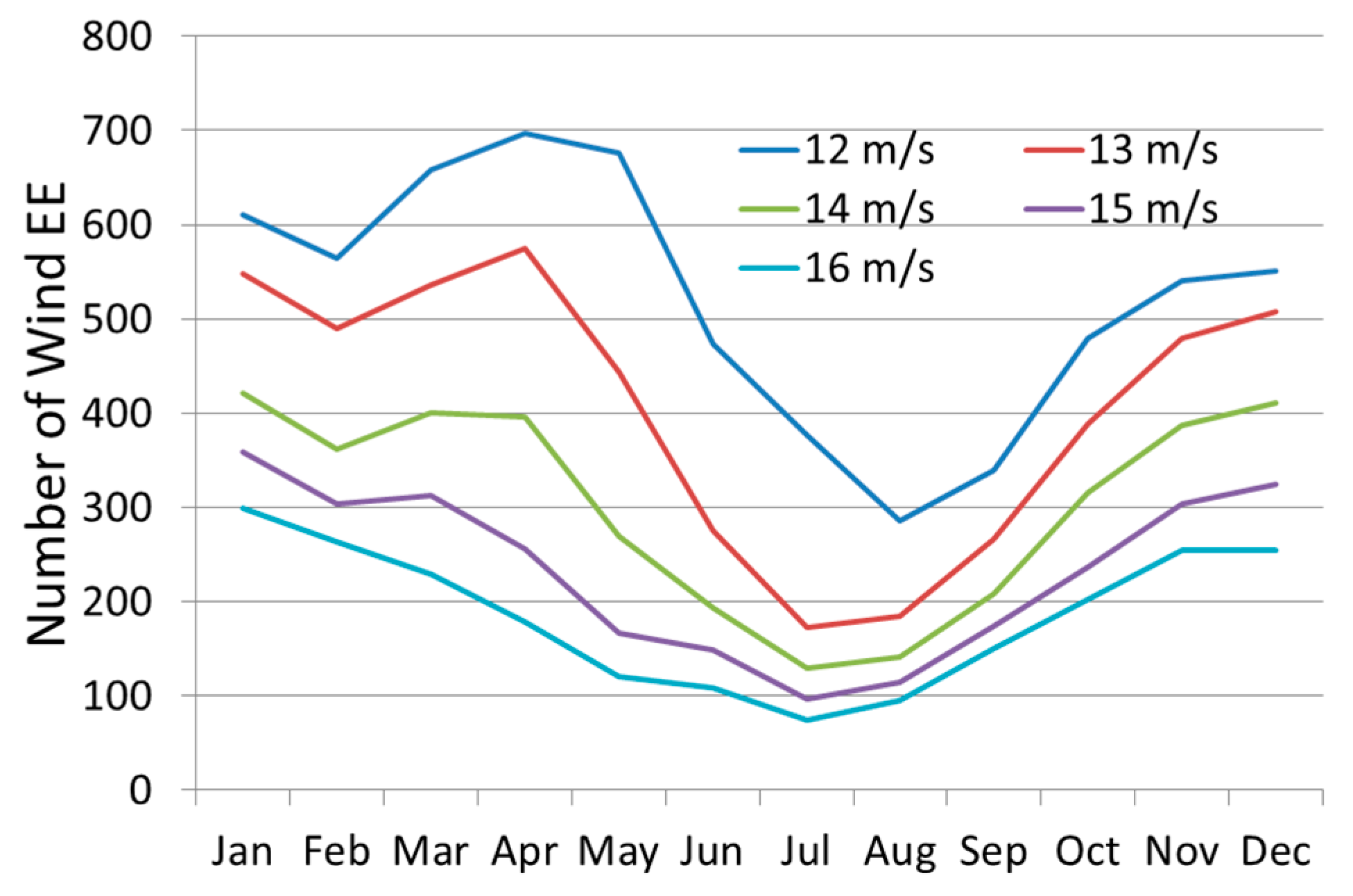
3.2. Quantitative Analysis of High Levels of Wave Energy Behavior in the GoM
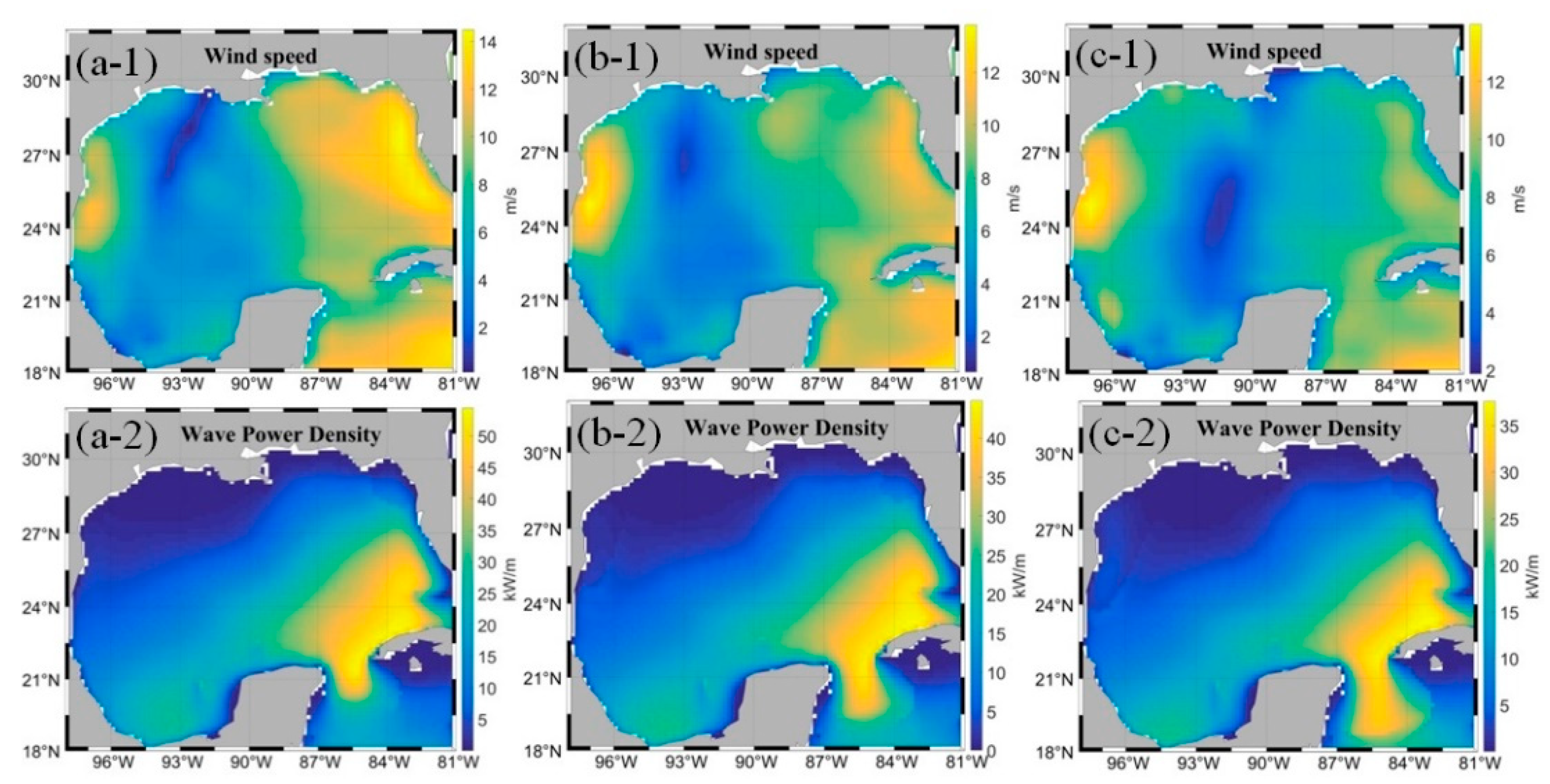
3.3. Low Levels Wave Energy in the GoM
4. Conclusions
Author Contributions
Funding
Institutional Review Board Statement
Informed Consent Statement
Data Availability Statement
Acknowledgments
Conflicts of Interest
References
- Cruz, J. Ocean Wave Energy: Current Status and Future Perspectives; Springer Science & Business Media: Berlin/Heidelberg, Germany, 2007. [Google Scholar]
- Holt, C. Energy from the Oceans. Phys. Educ. Lond. 2007, 42, 432. [Google Scholar] [CrossRef]
- Sawin, J.; Seyboth, K.; Sverrisson, F.; Adib, R.; Murdock, H. Renewables 2017 Global Status Report—REN21; REN21 Secretariat: Paris, France, 2017. [Google Scholar]
- Coe, R.G.; Neary, V.S. Review of methods for modeling wave energy converter survival in extreme sea states. In Proceedings of the 2nd Marine Energy Technology Symposium, METS2014, Seattle, WA, USA, 15–18 April 2014. [Google Scholar]
- Pelc, R.; Fujita, R.M. Renewable energy from the ocean. Mar. Policy 2002, 26, 471–479. [Google Scholar] [CrossRef]
- Astariz, S.; Iglesias, G. The economics of wave energy: A review. Renew. Sustain. Energy Rev. 2015, 45, 397–408. [Google Scholar] [CrossRef]
- Blummarch, P.A. Setback for Wave Power Technology. New York Times. 16 March 2009. Available online: https://www.nytimes.com/2009/03/16/ (accessed on 16 March 2016).
- Levitan, D. Why Wave Power Has Lagged Far behind as Energy Source. Yale Environment 360. Available online: https://e360.yale.edu-/feature/why_wave_power_has_lagged_far_behind_as_energy_source/2760 (accessed on 20 February 2015).
- Özger, M.; Şen, Z. Return period and risk calculations for ocean wave energy applications. Ocean. Eng. 2008, 35, 1700–1706. [Google Scholar] [CrossRef]
- Tiron, R.; Mallon, F.; Dias, F.; Reynaud, E.G. The challenging life of wave energy devices at sea: A few points to consider. Renewable and Sustainable Energy Rev. 2015, 43, 1263–1272. [Google Scholar] [CrossRef]
- Chawla, A.; Spindler, D.; Tolman, H. 30 Year Wave Hindcasts Using WAVEWATCH IIIR c with CFSR Winds Phase. NOAA/NWS/NCEP/MMAB, Maryland USA; National Oceanic and Atmospheric Administration. Environmental Modeling Center, Marine Modeling and Analysis Branch: Silver Spring, MA, USA, 2012.
- Penalba, M.; Ulazia, A.; Ibarra-Berastegui, G.; Ringwood, J.; Sáenz, J. Wave energy resource variation off the west coast of Ireland and its impact on realistic wave energy converters’ power absorption. Appl. Energy 2018, 224, 205–219. [Google Scholar] [CrossRef]
- Reguero, B.G.; Losada, I.J.; Méndez, F.J. A global wave power resource and its seasonal, interannual and long-term variability. Appl. Energy 2015, 148, 366–380. [Google Scholar] [CrossRef]
- Gu, C.; Li, H. Review on Deep Learning Research and Applications in Wind and Wave Energy. Energies 2022, 15, 1510. [Google Scholar] [CrossRef]
- Falnes, J. A review of wave-energy extraction. Mar. Struct. 2007, 20, 185–201. [Google Scholar] [CrossRef]
- Rusu, E. Evaluation of the wave energy conversion efficiency in various coastal environments. Energies 2014, 7, 4002–4018. [Google Scholar] [CrossRef] [Green Version]
- Bozzi, S.; Archetti, R.; Passoni, G. Wave electricity production in Italian offshore: A preliminary investigation. Renew. Energy 2014, 62, 407–416. [Google Scholar] [CrossRef]
- Stoutenburg, E.D.; Jenkins, N.; Jacobson, M.Z. Power output variations of co-located offshore wind turbines and wave energy converters in California. Renew. Energy 2010, 35, 2781–2791. [Google Scholar] [CrossRef]
- Haces-Fernandez, F.; Li, H.; Ramirez, D. A layout optimization method based on wave wake preprocessing concept for wave-wind hybrid energy farms. Energy Convers. Manag. 2021, 244, 114469. [Google Scholar] [CrossRef]
- Chakraborty, T.; Majumder, M. Impact of extreme events on conversion efficiency of wave energy converter. Energy Sci. Eng. 2020, 8, 3441–3456. [Google Scholar] [CrossRef] [Green Version]
- Chakraborty, T.; Majumder, M.; Khare, A. Application of AHP-VIKOR and GMDH framework to develop an indicator to identify utilisation potential of wave energy converter with respect to location. Int. J. Spatio Temporal Data Sci. 2019, 1, 98–113. [Google Scholar] [CrossRef]
- Chakraborty, T.; Majumder, M. Application of statistical charts, multi-criteria decision making and polynomial neural networks in monitoring energy utilization of wave energy converters. Environ. Dev. Sustain. 2019, 21, 199–219. [Google Scholar] [CrossRef]
- Gu, C.; Li, H. Wave Power Density Hotspot Distribution and Correlation Pattern Exploration in the Gulf of Mexico. Sustainability 2022, 14, 1158. [Google Scholar] [CrossRef]
- Neshat, M.; Mirjalili, S.; Sergiienko, N.Y.; Esmaeilzadeh, S.; Amini, E.; Heydari, A.; Garcia, D.A. Layout optimisation of offshore wave energy converters using a novel multi-swarm cooperative algorithm with backtracking strategy: A case study from coasts of Australia. Energy 2022, 239, 122463. [Google Scholar] [CrossRef]
- Amrutha, M.M.; Kumar, V.S. Evaluation of a few wave energy converters for the Indian shelf seas based on available wave power. Ocean. Eng. 2022, 244, 110360. [Google Scholar] [CrossRef]
- Naeem, M.; Jamal, T.; Diaz-Martinez, J.; Butt, S.A.; Montesano, N.; Tariq, M.I.; De-La-Hoz-Valdiris, E. Trends and future perspective challenges in big data. In Advances in Intelligent Data Analysis and Applications; Springer: Singapore, 2022; pp. 309–325. [Google Scholar]
- Nastasi, B.; Markovska, N.; Puksec, T.; Duić, N.; Foley, A. Renewable and sustainable energy challenges to face for the achievement of Sustainable Development Goals. Renew. Sustain. Energy Rev. 2022, 157, 112071. [Google Scholar] [CrossRef]
- Haces-Fernandez, F.; Martinez, A.; Ramirez, D.; Li, H. Characterization of wave energy patterns in Gulf of Mexico. In Proceedings of the IISE 2017 Annual Conference, Pittsburgh, PA, USA, 20–23 May 2017; pp. 1532–1537. [Google Scholar]
- Haces-Fernandez, F.; Ramirez, D.; Li, H. Wave Energy Characterization and Assessment in the U.S. Gulf of Mexico, East and West Coasts with Energy Event Concept. Renew. Energy 2018, 123, 312–322. [Google Scholar] [CrossRef]
- Jacobson, P.T.; Hagerman, G.; Scott, G. Mapping and Assessment of the United States Ocean Wave Energy Resource; (No. DOE/GO/18173-1); Electric Power Research Institute: Washington, DC, USA, 2011. [Google Scholar]
- Gadad, S.; Deka, P.C. Offshore wind power resource assessment using Oceansat-2 scatterometer data at a regional scale. Appl. Energy 2016, 176, 157–170. [Google Scholar] [CrossRef]
- Aderinto, T.O.; Haces-Fernandez, F.; Li, H. Design and Potential Application of Small Scale Wave Energy Converter—ASME International Mechanical Engineering Congress and Exposition. Energies 2017, 6, V006T08A084. [Google Scholar] [CrossRef]
- Haces-Fernandez, F. Investigation on the Possibility of Extracting Wave Energy from the Texas Coast. Master’s Thesis, Texas A&M University-Kingsville, Texas, TX, USA, 2014. [Google Scholar]
- Haces-Fernandez, F.; Li, H.; Ramirez, D. Assessment of the Potential of Energy Extracted from Waves and Wind to Supply Offshore Oil Platforms Operating in the Gulf of Mexico. Energies 2018, 11, 1084. [Google Scholar] [CrossRef] [Green Version]
- Hsu, C.T.; Wu, H.Y.; Hsu, E.Y.; Street, R.L. Momentum and energy transfer in wind generation of waves. J. Phys. Oceanogr. 1982, 12, 929–951. [Google Scholar] [CrossRef] [Green Version]
- Masuda, A. Nonlinear energy transfer between wind waves. J. Phys. Oceanogr. 1980, 10, 2082–2093. [Google Scholar] [CrossRef] [Green Version]
- Tolman, H.L. User Manual and System Documentation of WAVEWATCH III TM Version 3.14; Technical note; MMAB Contribution 276, no. 220, May 2009. Available online: https://polar.ncep.noaa.gov/mmab/papers/tn276/MMAB_276.pdf (accessed on 20 January 2022).
- Whitford, D.J. Teaching ocean wave forecasting using computer-generated visualization and animation-Part 1: Sea forecasting. Comput. Geosci. 2002, 28, 537–546. [Google Scholar] [CrossRef]
- Appendini, C.M.; Urbano-Latorre, C.P.; Figueroa, B.; Dagua-Paz, C.J.; Torres-Freyermuth, A.; Salles, P. Wave energy potential assessment in the Caribbean Low Level Jet using wave hindcast information. Appl. Energy 2015, 137, 375–384. [Google Scholar] [CrossRef]
- Available online: https://polar.ncep.noaa.gov/waves/wavewatch/ (accessed on 20 January 2022).
- Guiberteau, K.L.; Liu, Y.; Lee, J.; Kozman, T.A. Investigation of developing wave energy technology in the Gulf of Mexico. Distrib. Gener. Altern. Energy J. 2012, 27, 36–52. [Google Scholar]
- McArthur, S.; Brekken, T.K. Ocean wave power data generation for grid integration studies. In Proceedings of the 2010 IEEE Power and Energy Society General Meeting, Minneapolis, MN, USA, 25–29 July 2010; pp. 1–6. [Google Scholar]
- Thorpe, T.W. A Brief Review of Wave Energy; Harwell Laboratory, Energy Technology Support Unit: London, UK, 1999. [Google Scholar]
- Mirzaei, A.; Tangang, F.; Juneng, L. Wave energy potential along the east coast of Peninsular Malaysia. Energy 2014, 68, 722–734. [Google Scholar] [CrossRef]
- Musial, W.D. Status of Wave and Tidal Power Technologies for the United States; National Renewable Energy Laboratory: Golden, CO, USA, 2008.
- Kamranzad, B.; Etemad-Shahidi, A.; Chegini, V. Sustainability of wave energy resources in southern Caspian Sea. Energy 2016, 97, 549–559. [Google Scholar] [CrossRef] [Green Version]
- Contestabile, P.; Ferrante, V.; Vicinanza, D. Wave energy resource along the coast of Santa Catarina (Brazil). Energies 2015, 8, 14219–14243. [Google Scholar] [CrossRef] [Green Version]
- Hagerman, G. Southern New England wave energy resource potential. In Building Energy; Tufts University: Boston, MA, USA, 2001. [Google Scholar]
- Spindler, D.M.; Chawla, A.; Tolman, H.L. An Initial Look at the CFSR Reanalysis Winds for Wave Modeling; Technical Note; Environmental Modeling Center-Marine Modeling and Analysis Branch—NOAA: College Park, MA, USA, 2011.
- Von Landesberger, T.; Bremm, S.; Andrienko, N.; Andrienko, G.; Tekusova, M. Visual analytics methods for categoric spatio-temporal data. In Proceedings of the 2012 IEEE Conference on Visual Analytics Science and Technology (VAST), Seattle, WA, USA, 14–19 October 2012; pp. 183–192. [Google Scholar]
- Li, S.; Dragicevic, S.; Castro, F.A.; Sester, M.; Winter, S.; Coltekin, A.; Cheng, T. Geospatial big data handling theory and methods: A review and research challenges. ISPRS J. Photogramm. Remote Sens. 2016, 115, 119–133. [Google Scholar] [CrossRef] [Green Version]
- Guillou, N. Estimating wave energy flux from significant wave height and peak period. Renew. Energy 2020, 155, 1383–1393. [Google Scholar] [CrossRef]
- Morim, J.; Cartwright, N.; Etemad-Shahidi, A.; Strauss, D.; Hemer, M. Wave energy resource assessment along the Southeast coast of Australia on the basis of a 31-year hindcast. Appl. Energy 2016, 184, 276–297. [Google Scholar] [CrossRef]
- Klemeš, J.J.; Kravanja, Z.; Varbanov, P.S.; Lam, H.L. Advanced multimedia engineering education in energy, process integration and optimisation. Appl. Energy 2013, 101, 33–40. [Google Scholar] [CrossRef]
- Mari, R.; Bottai, L.; Busillo, C.; Calastrini, F.; Gozzini, B.; Gualtieri, G. A GIS-based interactive web decision support system for planning wind farms in Tuscany (Italy). Renew. Energy 2011, 36, 754–763. [Google Scholar] [CrossRef]
- Baban, S.M.; Parry, T. Developing and applying a GIS-assisted approach to locating wind farms in the UK. Renew. Energy 2001, 24, 59–71. [Google Scholar] [CrossRef]
- Blok, C.; Kobben, B.; Cheng, T.; Kuterema, A.A. Visualization of relationships between spatial patterns in time by cartographic animation. Cartogr. Geogr. Inf. Sci. 1999, 26, 139–151. [Google Scholar] [CrossRef]
- Ramírez, G.; de Dios, J.; Mejía Fuentes, O.I.; Menjívar Pino, P.J. Evaluación del Potencial Energético del Oleaje en las Costas de El Salvador. Ph.D. Thesis, Universidad de El Salvador, San Salvador, El Salvador, 2013. [Google Scholar]
- Sierra, J.P.; González-Marco, D.; Sospedra, J.; Gironella, X.; Mösso, C.; Sánchez-Arcilla, A. Wave energy resource assessment in Lanzarote (Spain). Renew. Energy 2013, 55, 480–489. [Google Scholar] [CrossRef]
- Alonso, R.; Solari, S.; Teixeira, L. Wave energy resource assessment in Uruguay. Energy 2015, 93, 683–696. [Google Scholar] [CrossRef]
- Neill, S.P.; Hashemi, M.R. Wave power variability over the northwest European shelf seas. Appl. Energy 2013, 106, 31–46. [Google Scholar] [CrossRef]
- Neill, S.P.; Lewis, M.J.; Hashemi, M.R.; Slater, E.; Lawrence, J.; Spall, S.A. Inter-annual and inter-seasonal variability of the Orkney wave power resource. Appl. Energy 2014, 132, 339–348. [Google Scholar] [CrossRef] [Green Version]
- Langodan, S.; Viswanadhapalli, Y.; Dasari, H.P.; Knio, O.; Hoteit, I. A high-resolution assessment of wind and wave energy potentials in the Red Sea. Appl. Energy 2016, 181, 244–255. [Google Scholar] [CrossRef]
- Commin, A.N.; French, A.S.; Marasco, M.; Loxton, J.; Gibb, S.W.; McClatchey, J. The influence of the North Atlantic Oscillation on diverse renewable generation in Scotland. Appl. Energy 2017, 205, 855–867. [Google Scholar] [CrossRef]
- Monforti, F.; Gonzalez-Aparicio, I. Comparing the impact of uncertainties on technical and meteorological parameters in wind power time series modelling in the European Union. Appl. Energy 2017, 206, 439–450. [Google Scholar] [CrossRef]
- Chen, J.; Yang, S.; Li, H.; Zhang, B.; Lv, J. Research on geographical environment unit division based on the method of natural breaks (Jenks). Int. Arch. Photogramm. Remote Sens. Spat. Inf. Sci. 2013, 3, 47–50. [Google Scholar] [CrossRef] [Green Version]
- Wong, M.S.; Zhu, R.; Liu, Z.; Lu, L.; Peng, J.; Tang, Z.; Chan, W.K. Estimation of Hong Kong’s solar energy potential using GIS and remote sensing technologies. Renew. Energy 2016, 99, 325–335. [Google Scholar] [CrossRef]
- Mellino, S.; Ulgiati, S. Mapping the evolution of impervious surfaces to investigate landscape metabolism: An Emergy–GIS monitoring application. Ecol. Inform. 2015, 26, 50–59. [Google Scholar] [CrossRef]
- Miller, A.; Li, R. A geospatial approach for prioritizing wind farm development in Northeast Nebraska, USA. ISPRS Int. J. Geo Inf. 2014, 3, 968–979. [Google Scholar] [CrossRef] [Green Version]

| Wind (m/s) | Wave Energy Events (kW/m) | ||||
|---|---|---|---|---|---|
| 25 | 35 | 55 | 75 | 100 | |
| 12 | 1430 | 1127 | 690 | 440 | 276 |
| 13 | 1209 | 1156 | 733 | 473 | 294 |
| 14 | 815 | 949 | 736 | 483 | 305 |
| 15 | 503 | 685 | 659 | 480 | 308 |
| 16 | 304 | 461 | 540 | 440 | 299 |
| Wind (m/s) | Wave Energy Events (kW/m) | ||||
|---|---|---|---|---|---|
| 25 | 35 | 55 | 75 | 100 | |
| 12 | 23% | 18% | 11% | 7% | 4% |
| 13 | 25% | 24% | 15% | 10% | 6% |
| 14 | 22% | 26% | 20% | 13% | 8% |
| 15 | 18% | 24% | 24% | 17% | 11% |
| 16 | 14% | 21% | 24% | 20% | 13% |
| Wind (m/s) | Data Type | Duration of Wind EE (h) | |||||||||||
|---|---|---|---|---|---|---|---|---|---|---|---|---|---|
| Jan. | Feb. | Mar. | Apr. | May | Jun. | Jul. | Aug. | Sep. | Oct. | Nov. | Dec. | ||
| 12 | Mean | 23 | 21 | 19 | 15 | 11 | 11 | 9 | 13 | 22 | 21 | 24 | 23 |
| Std | 27 | 26 | 26 | 19 | 14 | 20 | 18 | 22 | 32 | 34 | 32 | 27 | |
| 13 | Mean | 18 | 17 | 15 | 11 | 9 | 11 | 11 | 15 | 20 | 19 | 19 | 18 |
| Std | 22 | 19 | 19 | 13 | 11 | 19 | 20 | 23 | 30 | 31 | 25 | 21 | |
| 14 | Mean | 17 | 15 | 13 | 9 | 7 | 10 | 10 | 14 | 19 | 17 | 16 | 16 |
| Std | 19 | 17 | 16 | 10 | 9 | 16 | 18 | 23 | 29 | 28 | 21 | 17 | |
| 15 | Mean | 14 | 13 | 11 | 8 | 6 | 9 | 9 | 14 | 18 | 17 | 15 | 14 |
| Std | 15 | 15 | 13 | 9 | 8 | 14 | 18 | 24 | 30 | 27 | 18 | 15 | |
| 16 | Mean | 11 | 10 | 10 | 7 | 5 | 8 | 8 | 14 | 16 | 15 | 13 | 12 |
| Std | 12 | 13 | 11 | 8 | 7 | 12 | 17 | 24 | 29 | 26 | 15 | 13 | |
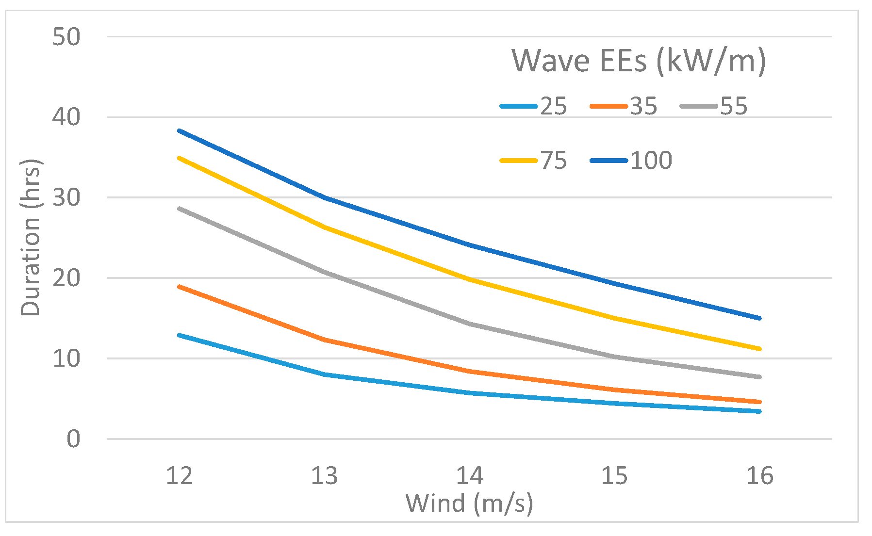
| Wind (m/s) | Wave Energy Events (kW/m) | ||||
|---|---|---|---|---|---|
| 25 | 35 | 55 | 75 | 100 | |
| 12 | 12.9 | 18.9 | 28.6 | 34.9 | 38.3 |
| 13 | 8.0 | 12.3 | 20.7 | 26.3 | 30.0 |
| 14 | 5.7 | 8.4 | 14.3 | 19.8 | 24.1 |
| 15 | 4.4 | 6.1 | 10.2 | 15.0 | 19.3 |
| 16 | 3.4 | 4.6 | 7.7 | 11.2 | 15.0 |
Publisher’s Note: MDPI stays neutral with regard to jurisdictional claims in published maps and institutional affiliations. |
© 2022 by the authors. Licensee MDPI, Basel, Switzerland. This article is an open access article distributed under the terms and conditions of the Creative Commons Attribution (CC BY) license (https://creativecommons.org/licenses/by/4.0/).
Share and Cite
Haces-Fernandez, F.; Li, H.; Ramirez, D. Analysis of Wave Energy Behavior and Its Underlying Reasons in the Gulf of Mexico Based on Computer Animation and Energy Events Concept. Sustainability 2022, 14, 4687. https://doi.org/10.3390/su14084687
Haces-Fernandez F, Li H, Ramirez D. Analysis of Wave Energy Behavior and Its Underlying Reasons in the Gulf of Mexico Based on Computer Animation and Energy Events Concept. Sustainability. 2022; 14(8):4687. https://doi.org/10.3390/su14084687
Chicago/Turabian StyleHaces-Fernandez, Francisco, Hua Li, and David Ramirez. 2022. "Analysis of Wave Energy Behavior and Its Underlying Reasons in the Gulf of Mexico Based on Computer Animation and Energy Events Concept" Sustainability 14, no. 8: 4687. https://doi.org/10.3390/su14084687
APA StyleHaces-Fernandez, F., Li, H., & Ramirez, D. (2022). Analysis of Wave Energy Behavior and Its Underlying Reasons in the Gulf of Mexico Based on Computer Animation and Energy Events Concept. Sustainability, 14(8), 4687. https://doi.org/10.3390/su14084687