Traffic Flow Prediction: An Intelligent Scheme for Forecasting Traffic Flow Using Air Pollution Data in Smart Cities with Bagging Ensemble

Abstract

Traffic flow prediction is the most critical part of any traffic management system in a smart city. It can help a driver to pick the most optimized way to their target destination. Air pollution data are often connected with traffic congestion and there exists plenty of research on the connection between air pollution and traffic congestion using different machine learning approaches. A scheme for efficiently predicting traffic flow using ensemble techniques such as bagging and air pollution has not yet been introduced. Therefore, there is a need for a more accurate traffic flow prediction system for the smart cities. The aim of this research is to forecast traffic flow using pollution data. The contribution is twofold: Firstly, a comparison has been made using different simple regression techniques to find out the best-performing model. Secondly, bagging and stacking ensemble techniques have been used to find out the most accurate model of the two comparisons. The results show that the K-Nearest Neighbors (KNN) bagging ensemble provides far better results than all the other regression models used in this study. The experimental results show that the KNN bagging ensemble model reduces the error rate in predicting the traffic congestion by more than 30%.

1. Introduction

Rapidly increasing economic activities in the whole world and ever-increasing population density caused roads to fill with more traffic and as a result, there is more congestion on roads. This congestion leads to air pollution which caused some serious health issues in urban areas according to the Harvard school of public health [1]. Air pollution from congested traffic in 83 nations urban areas contributes to more than 22,000 deaths each year which costs the health system a whopping 18 billion dollars according to Harvard School of Public Health. Traffic congestion also causes the waste of time and fuel along with that it also costs in terms of economics. It affects job growth because of traffic congestion getting up to 35 to 37 h per commute per year according to Bloomberg [2]. Due to road traffic, there is severe air pollution in urban areas which causes problems such as smog and carbon monoxide (CO). It is considered a major threat to clean air in the UK and other industrialized states. Road traffic emissions contain harmful chemicals such as CO, sulfur dioxide (SO${}_2$), nitrogen dioxide (NO${}_2$) and others which pollute the atmosphere resulting in poor health conditions [3].

Pollution and decreasing air quality due to road congestion is the main reason for high mortality rates in urban areas of big cities according to the World Health Organization (WHO) [4], almost 40 million people in 115 largest cities of EU (European Union) are unshielded from ever exceeding WHO air quality directives for at least one pollutant. A lot of cities are addressing this issue by using different sensors alongside the roads to measure traffic flow and pollutants in the air caused because of traffic congestion. The more time vehicles are in congestion, the high percentage of fuel is used which results in high vehicular emissions of carbon dioxide (CO${}_2$), CO, hydrocarbons (HC), and (NO${}_2$) [5]. These traffic pollutants cause many diseases such as lung cancer, cardiovascular diseases, and so forth. They cause many respiratory diseases as well and also become the reason for many kinds of infections. If a driver can be notified in advance about the roads without congestion to the destination they want to reach or shorten the traveling time to adjust to less congested periods then traffic jams can be avoided. This can cause a reduction in air pollutants and improved health conditions.

Many studies have been conducted before to predict or model air quality using traffic data, for example, ref. [6]. The study mainly used the long short-term memory (LSTM) approach to predict (O${}_2$), (PM${}_{2.5}4$), (NO${}_2$), and (CO${}_{2}4$) concentrations which are thought to be faster than many Deep Learning (DL) models that can be used. Different parameters and elements such as meteorological conditions, vehicular emissions, pollutant levels, and the data of traffic were used in 5 different combinations; However, they did not consider the high volume of traffic. If it is known in advance by a person that what are the traffic conditions of the roads that are taking them to their destinations, the traveling of that person will be less stressful and more comfortable. The traffic management system is considered the main component of the smart city. One of the most important components in traffic management services is smart mobility. Several health issues are caused by traffic jams in many urban cities. Another major issue is the loss of time caused by being stuck in a traffic jam. To provide the people with the privilege to use the less congested roads, a smartly managed congested strategy is used and as a result, it becomes less vulnerable to the effects of traffic-related health because of less density of air pollutants. Predicting the road traffic effectively and efficiently has become a big challenge because of the heavy intercity and intracity traffic flow and the changing behavior of roads networks. Smart congestion reduction system which is part of traffic management systems in smart cities plays a pivotal role in mobility, ease of travel, and growth of urban cities. According to this research, air pollutants play an important role in traffic intensity prediction. By using air pollutants data, road traffic can be predicted precisely. In all previous studies, air pollution is forecasted using traffic data.

A small number of researchers have investigated forecasting or improving traffic congestion, most of them did not take into account the use of air pollutants to predict traffic congestion or density. Along with that, they have used traditional statistical techniques to approach this problem when now there are advanced neural networks to solve such problems more precisely. The main cause of the high density of air pollutants during traffic congestion is the high volume of vehicles. So, air pollutant data can be used to predict the number of vehicles on the road that would ultimately be used to conclude whether the road is congested or not. Because in modern days a high volume of traffic can be seen on highways which ultimately causes high amounts of air pollutants and thus the reason for using air pollutants data to predict the number of vehicles.

The main purpose of this research is to get aware of the fact that whether this method can be proved successful to tackle with traffic congestion problem. Whether it is effective and provides the desired results. Along with that if models used in this study perform well and help in the reduction of different kinds of sensors used on roads to monitor traffic. These sensors cost a lot of resources to maintain and use. If most specific task-based sensors can be skipped and instead could use sensors that can be generally used for large and complex urban traffic. It could mean that rather than a complex mesh of traffic sensors model would be able to use only the data related to air pollution to predict traffic congestion. In this study, a new scheme is proposed to predict traffic on a road by splitting the data and feeding them into 10 different models which are combined using an ensemble technique. Three different ensemble models are used to conduct the analysis. There are 10 different models and for each of them, different regression models are used. This study is detailed in the experiment section. Four different evaluation metrics were used to conduct this experiment which were R-squared error (R2), Mean Absolute Error (MAE), Root Mean Square Error (RMSE), Relative Absolute Error (RAE).

2. Related Work

In this section different schemes are discussed that were previously used for traffic prediction which is the following:

2.1. Deep Learning

There are many subfields in Machine Learning (ML), one of them is DL. It is a domain of Artificial Intelligence (AI) which comprises algorithms that are based upon learning and improving on their own with experience. While simpler concepts are used in ML but DL is something that uses Artificial Neural Networks (ANN) for its working. ANNs are like a human brain and are designed to replicate the thinking and learning process of humans. The improvements in computing power and the emergence in the field of Big Data tools have helped build sophisticated and complicated neural networks. It has greatly helped to observe and learn the patterns by the computers and to solve complex problems way faster than humans. Aided image classification, language translation, speech recognition to name a few were improved by using DL. By using DL, many fields have been improved which were pattern recognition problems, speech recognition, image classification, and without the assistance of the human.

There are various layers to compose the ANN, these layers make use of DL. A type of network with which every layer can learn complex patterns to make the sense of the image and text is known as Deep Neural Network (DNN). It is a field in ML that is growing rapidly and is representing a truly revolutionary technology that is being used by an ever-increasing number of companies to build business models.

2.1.1. Long Short Term Memory

In order to develop a model to learn order dependence in the sequence forecasting problem, LSTM is used. There are many complex problem fields for which it is used such as machine translation, speech recognition, and so forth. One of the complex fields of DL is LSTMs. The authors of [7] used a DL approach that extracts the features of traffic, with the help of its temporal features and graph convolution by using LSTM cells in order to have both predictions short or long term. GPS (sparse trajectory) data extracted from a service related to the ride-hailing known as Didi from cities of Chengdu and Xi’an in China was used, however, air pollution data were not considered. In [8], the authors have developed a residual graph convolution, also known as the residual graph convolution long short-term memory (RGC-LSTM) model. That was used for the prediction over the data related to spatial-temporal. It was used at the speed of ten minutes. The data were extracted from two sources which are Shanghai, China, and Caltrans Performance Measurement System (PeMS) traffic flow data. Fewer features were used and air pollution data were not considered which is the reason why it has a high error rate. Convolutional LSTM was used in [9] which is a neural network architecture. It is being used for the forecasting of multi-lane short-term traffic. The importance to apply multiple features to predict the conditions of the traffic was highlighted. Downstream/upstream traffic and the ways between neighboring lanes were considered. The rolling-prediction way is the forecasting of multiple time-step traffic. The data used was extracted from the PeMS. In every thirty seconds, the data were collected from more than thirty-five thousand individual single-lane loop detectors, these were put in place state-wide in freeway systems across California. The flow and speed of traffic were used to forecast it and that is why the error was considerably high.

In paper [10], authors have made use of a Stacked Bidirectional and Unidirectional LSTM (SBU-LSTM) network architecture to help in designing a neural network scheme in order to predict the traffic state. LSTM is being used as the main component of the scheme. To take note of the forward and backward temporal dependencies the bidirectional LSTM (BDLSM) was used in spatiotemporal data. For the purpose to avoid the values that are missing in spatial-temporal data, a data imputation process was proposed. This process is proposed in the LSTM structure (LSTM-I). In order to reduce the values that are missing and to facilitate the forecasting of traffic, it was used to develop an imputation unit. SBU-LSTM structure contains the bidirectional part of LSTM-I that was included in it. To perform the experiment two real-world datasets were used based on network-wide traffic state. The experiments were further published to facilitate the research and development in traffic forecasting. Results of forecasting of different types of multi-layer LSTM or BDLSTM models were assessed. The SBU-LSTM scheme was proposed with the help of experimental results, especially the two-layer BDLSTM network. It showed good performance on network-wide traffic forecasting, however, MAE and RMSE values were way higher. Graph attention mechanism was used in [11] to extracts the spatial dependencies between road segments. Along with that, an LSTM network to extract features related to the temporal domain was introduced. PeMSD7 dataset collected by the California Department of Transportation was used, however, air pollution data were not considered.

2.1.2. CNN

The model presented in [11] is based on Convolution Neural Network (CNN) and DL architecture. This model is related to the prediction of the traffic in the short-term flow. In this scheme, the Spatio-Temporal Feature Selection Algorithm (STFSA) was being used to resolve the most efficient input data time and the lags and amounts of spatial data. From the actual data, the selected Spatio-temporal traffic flow features were obtained. They were then transformed into a two-dimensional matrix. To build a model for prediction CNN learned the available features. The dataset they used was from the Washington State Department of Transportation (WSDOT) on the theI-5 Freeway in Seattle, WA, USA.

The authors of [12] propose a novel DL technique named mapping to cube scheme for network-wide urban traffic prediction. On the real Taxi data, the experiments were performed. It was the data taken from the real taxi Graphical positioning System (GPS) vehicle data. It confirms the effectiveness and the accuracy of a model which combines 3-Dimensional Convolutional Networks (C3D). By using the CNNs and Recurrent Neuron Networks (RNNs), which is called the CRC3D method a mixture of CNN-RNNs and C3Ds. The dataset used was taken from the municipality of Shenzhen, China, however, due to fewer data, the model is not much robust. Graph Convolutional Neural Network (GCNN) and LSTM based transfer learning techniques on a large real-world image and video data were used, however, work was not done on reducing the time for video processing along with that air pollution data were not considered. The paper [13] developed and used an extended version of Spatiotemporal K-Nearest Neighbors (SKNN) which is a dynamic transformed into STKNN model D-STKNN for traffic forecasting in short periods. Thus, making use of the non-stationary spatiotemporal model of the traffic flow on the road. Datasets related to vehicular speed processed by the roads in Beijing, China, and expressways in California, U.S.A were used. Attention Temporal Graph Convolutional Network (A3T-GCN) was used [14] which simultaneously captures global temporal dynamics and spatial relationships in traffic flow. The A3T-GCN model extracts the short-term direction by making use of the gated recurrent units and learns the spatial reliance using the road network topology via the graph convolutional Network. SZ-taxi and Los-loop datasets were used to carry out experiments. Limited data were used which can be a problem in generalizing. The authors of [11] proposed the model in spatial-temporal graph inception residual network (STGIResNet) was used. For the network-based traffic prediction, STGIResNet was used. In the model, multiple Spatial-Temporal Graph Convolution (STGC) operators, residual learning, and the inception structure were combined. Experiments were conducted on a dataset related to car-hailing traffic at ten to thirty and thirty to sixty minutes intervals. The study was performed on a large network of roads in a Chinese city. The value of RMSE was high in the paper because the data of air pollution was not considered by them.

2.2. Machine Learning

There are different fields of AI, one of them is ML. ML approaches are used to replicate the decision-making behavior of humans by using different models and algorithms that can learn based on experience and the data provided to them. ML models learn gradually and make improvements with time and their learning rate based on data provided to them.

2.2.1. Naïve Bayes

Naïve Bayes is a technique for developing classifiers that label class to feature instances, which are given as vectors of feature values, where the labels of class are determined from some finite set of values.

Naïve Bayes classifier scheme was used in [15] to model this causation connection. The field survey data and Scikit-learn library of python were used. Data were divided into test and train datasets. The proposed model has 72.25% and 85.03% accuracy in training and testing sets. The RMSE was 0.46 and the MAE of the model was 0.28. The Naïve Bayes classifier model results show good performance to assess the effect of weather conditions on traffic. The purpose of the approach was to develop an Advance Traffic Management System (ATMS) and Advanced Traveller Information System (ATIS) for the city of Dhaka. As result, the drivers can decide on their own to take routes having less congestion which will reduce congestion effectively.

2.2.2. KNN

The KNN algorithm is based upon supervised learning that solves a classification or regression problem it does this by assuming that the things that are similar exist in close proximity or it can be said as the same things are close to one another.

The authors of [16] tackle the problem of the model architectures that is fixed and is quality-wise vague in terms of both space and time, dependent relationships. An adaptive space and time-based K Nearest-Neighbor model (adaptive-STKNN) for the prediction of the traffic flow in short periods was proposed. The model completely takes into account the spatial heterogeneity of city traffic based upon adaptive spatial neighbors, time windows, spatiotemporal weights, and other variables. Initially, the size of spatial neighbors and the lengths of time windows for each road patch to check traffic influence by making use of cross-correlation and autocorrelation functions were obtained. After that, adaptive spatiotemporal weights were presented into the distance functions to make every candidate neighbor search approach more efficient. Then adaptive spatiotemporal to show the continuous changes in the conditions of vehicle traffic was developed, including the number of candidate neighbors and the weight allocation variable in the predictive module. In the end, the adaptive-STKNN model was evaluated, and two datasets were used for it based on vehicular speed which was gathered on expressways in California, USA, and on city roads in Beijing, China. Kernel KNN scheme was proposed in [17]. It was for the traffic states on the road in accordance with the time series. Firstly, representative data related to traffic state on road was accumulated. It was to develop the running characteristics of traffic on the road with the reference sequences. After this step, the kernel module was constructed for the data of time series related to traffic state on the roads. Compared and matched was performed on the data sequences which were from the referenced and the current data. It was related to road traffic state. Depending on the closest referenced traffic states on the road were selected and the road traffic states were forecasted and a lot of typical links of roads in Beijing were included for a series of experiments. Although the model was not generic.

2.3. ARIMA

Auto Regressive Integrated Moving Average (ARIMA) is a set of schemes that explains any time series problem by means of its previous values, which are the lags and the error of lagged forecast of the model. This is helpful for the model in order to be able to predict future values. It is a time series problem that is non-seasonal and has patterns in it. It can not be said as random. White noise is learnt by using the ARIMA models.

The paper [18] used the combination of Kohonen and ARIMA technique where Kohonen was mapped and declared as it can self-organize itself, as the first classifier; a separately trained ARIMA technique is being used for each class that is connected with it. Leveraging a Kohonen map that is hexagonal in look simplifies the issue through which the classes can be defined. Precision performance was immensely improved with the use of the jobs of classification that are based on functional approximation and the unique isolation, by comparing it to a backpropagation neural network or a single ARIMA model. This model is presented by producing a prediction of the flow of traffic, on the different time durations such as half an hour and one hour, for a French motorway. The performance of this model was related to other layered models that have been used. Only two to four smaller classes were needed. Less number of classes is the indication that it can be easily retained in order to make the long-term changes in the density of the traffic. It also indicates that it is readily transformable. Auto-regressive integrated moving average scheme was used in [19] to predict traffic based on measurements taken online. After using AMIRA, a bandwidth provisioning model was used which assigns bandwidth depending upon the traffic predictions. The problem was modeled as a fractional knapsack problem for which a greedy algorithm was used to find an approximate solution. By using simulations on real-world datasets, a pattern was found that technique can increase the bandwidth for the real-time traffic class and also guarantee adequate service quality for the non-real traffic class as well so generalizing technique while maximizing the utilization of resources.

2.4. Ensemble Techniques

The ensemble models are a bunch of techniques that use different models or learning algorithms to generate optimal predictive models that are optimal. This final model produces far better results than those base learners if they are taken alone. There are also other uses of ensemble learning that select the most important features, data fusion, and so forth. Ensemble techniques have three primary types which are bagging, boosting, and stacking.

2.4.1. Boosting

This technique is mainly used in supervised learning which involves two steps, first bootstrapping and the second aggregation. In bootstrapping random samples are derived from a dataset by using replacement techniques which are then fed to the base learner. Afterward, the base learner is trained on those samples to complete the procedure. After bootstrapping aggregation was used in which outputs were used from the base learners and combine. Finally, the goal is to improve the accuracy while reducing the variance to a large extent. For example, Random Forest (RF) where the predictions made by decision trees are taken parallelly. Multivariate GBRT was proposed in [11] which realizes parallel more than one output by taking into account the relationships of the outputs which have not been completely considered in the approaches used before. At the five minutes aggreged time the data of the traffic was detected. In order to perform this task, the PeMS used three-loop detectors in the US101-N freeway. Support Vector Regressor (SVR) technique was applied as the reference. Assessments of three models were based on three requirements, which are accuracy of the prediction, stability of the prediction, and the time of the model to predict. The results of experiments conclude that by directly using GBRT and multivariate GBRT, the prediction can be made higher than to SVR. GBRT by making use of iterated strategy results in a decent accuracy of prediction in short-step-ahead prediction and log-step-ahead the accuracy of precious decreases significantly. Best stability is provided by Multivariate GBRT. That means that the higher reliability is provided in multi-step-ahead prediction than the iterated GBRT. The worst of them all stability is provided by the GBRT. The issue with the technique is that it is not generic and their RMSE and MAE error is high.

The authors of [20] proposed a gradient boosting technique along with the hierarchical reconciliation to predict the traffic density in short term. A lot of emphases was made on 3 of the characteristics with significant importance, related to the traffic flow which are the spatial and temporal models, the interactions between these two models, and the traffic density dynamics of different spatial at aggregation levels. The proposed framework’s performance was checked and tested by comparing it with SARIMA, kalman filter model, and RF techniques were also used along with that three different datasets were used. Information in the large datasets is learned by using the technique of gradient boosting that offers automated and highly flexible ways to learn. This information is very beneficial for traffic forecasting density in a big road network. It is forecasted at longer horizons, however, pollution data were not used.

Boosting ensemble technique was used in [21] to boost the results of one regression model and then passed it through the second regression which improves results along with that different regression models were compared by extensive comparative analysis. The dataset that was used is available publicly, it is the dataset that consists of the information on the Pulse Aarhus City. Various techniques such as RMSE, MAE, and Mean Absolute Percentage Error (MAPE) were employed. They were used for the evaluation of techniques used in the study, however, boosting was used to tackle the problem of predicting the traffic intensity using pollution data but the problem in using boosting is that it suffers from outliers because every model must fix errors in the previous model. As result, the technique is too reliant on outliers. Another reason that results suffered and boosting cannot be scaled up to a certain level reason being is that every model bases its correctness on the previous model result making the technique difficult to scale. Experiments were made with fewer combinations of models using the proposed technique. The error rate could be improved further.

2.4.2. Stacking

In comparison to bagging and boosting which make use of homogeneous weak models for ensemble, stacking leverages heterogeneous weak models which learn side by side. After learning it merges them by training a meta-learner which outputs a prediction based upon different weak modes predictions. The way a meta learner works is it inputs the predictions made by a weak learner as features and the target is ground truth values given in data. It learns to combine the predictions made by weak learners as features to make a better prediction. 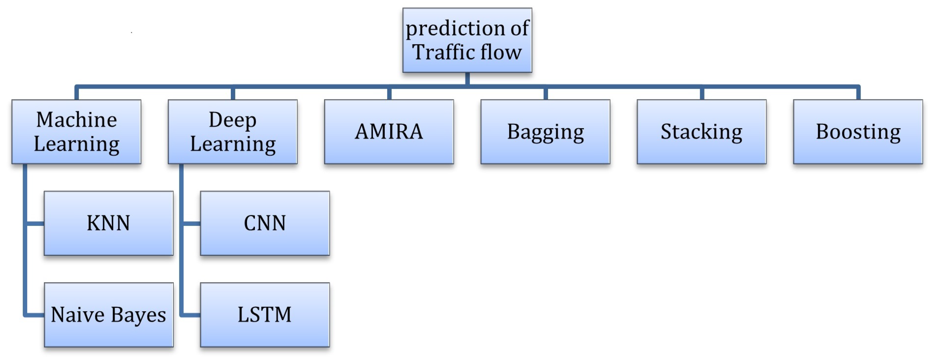RNN-based schemes were used [10] in which a technique was used to include RNN and its variants to predict traffic flow. A stacked architecture was proposed which is a network called unidirectional LSTM and stacked bidirectional which assisted in the design of neural network architecture for prediction of traffic state and is one of the most important components of this technique. The BDLSM model was used to get backward and forward temporal relationships in the spatiotemporal data. It was for taking care of the values that were missing in spatial-temporal data, a data imputation scheme was used in the LSTM model by developing an imputation part to find the values that were missing and help in traffic flow prediction. In the SBU-LSTM structure, the bidirectional part of LSTM was included. The datasets used were based on real-world data. These were two network-wide datasets that were based on the traffic state to conduct the study. It was published as well so that it can help in the prediction studies related to the flow of traffic. More than one type of multi-layer LSTM or BDLSTM was evaluated. The results show that the proposed technique provided great performance, especially the two-layer BDLSTM network, which could achieve a fair performance for the prediction of traffic flow. RMSE value is too high, and pollution data were not considered.A chart which shows traffic flow Prediction done by different approaches is given in Figure 1.

The authors of [22] used a stacked autoencoder to forecast the traffic flow but there are some drawbacks that exist in the technique. A sample replication strategy was used to train multiple stacked auto-encoders and an adaptive boosting technique to ensemble the autoencoders trained. The method hugely impacted the improvements in the predictions of the traffic flow, however, no comparative analysis was performed. A review of previously used methods is given in

Table 1. A review of previously used methods.

Schemes Used	Contribution	Deficiencies	Evaluation Methods	Dataset Used
STGI-ResNet [8]	A novel, Spatial-temporal DL architecture for large-scale traffic prediction	Only 1-month data are considered	RMSE, MAE, NRMSE, MAPE	Traffic Dataset from Didi GAIA initiative Chengdu, China
LSTM + BDLSTM [10]	Captured backward and forward dependencies that are Temporal in Spatiotemporal data	Only compared with 1 model	MAP, MAE, RSME	LOOP-SEA Dataset, PeMS-BAY Dataset
CNN+RNN+C3D [12]	Worked on Large-scale traffic flow prediction	Did not include pollution data features, only compared with 2 models	RMSE, Accuracy, Recall	Traffic flow dataset of Shenzhen, China
A3T-GCN [14]	Improved results over baselines on SZ-taxi and Los-loop datasets	Haven’t considered pollution attributes and the error rate is high	RMSE, MAE, Accuracy, R-2, var	The taxi trajectory dataset (SZ-taxi) Shenzhen City, loop detector dataset Los Angeles
STKNN [16]	Proposed technique to consider traffic spatial heterogeneity	Only worked on short-term traffic prediction	MAE, MAPE, RMSE	traffic data from PeMS, Floating car speed data from Beijing
Kernel KNN [17]	Traffic states were predicted accurately	Only two features speed and volume were used	MAE, MAPE, RMSE	Microwave sensors data collected by RTRCS
CNN + STFSA [23]	Considered spatial and temporal attributes of traffic flow	Small dataset and error rate is high	MAP, MAE	Washington State Department of Transportation (WSDOT) dataset
LSTM + MDC [24]	Proposed Novel DL based network for traffic prediction	Less features to used and did not include pollution features	MAE, RMSE, MAPE	traffic data from PeMS
GCNN [25]	spatiotemporal video prediction along with transfer learning	Only video data are used	MAE	Indian Driving Dataset (IDD)
Multivariate RNN [26]	Better results as compared to other studies done using cameras	Only Camera generated data are used	MSE, MAE, RMSE	London’s traffic camera images

.

2.4.3. Bagging

This is an ensemble technique that takes homogeneous weak models, learns them in isolation from each other, and then combines them by means of a deterministic averaging scheme. In bagging several independent learners are used to make predictions on data and then the average of the predictions is taken to train a model which has lower variance. In practice, it is not possible to fitfully isolated learners as that would require more data. As a result, fair approximate characteristics of bootstrap sampling are relied upon to train good models that are independent.

The authors of [27] used ensemble learning to forecast traffic in which characteristics of multitask learning and ensemble learning were combined. In traditional traffic density forecasting techniques, a single task learning model might be avoiding important information embedded in some related tasks. So, in contrast to that multitask learning integrates patterns from related tasks. In recent times the developments in ensemble learning-based traffic forecasting have improved. The method which is named MTLBag is a mixture of multitask learning and a well-known ensemble learning technique bagging, for traffic flow prediction. By using neural network learners first, the advantages of using multitask learning were presented in comparison to single-task learning for the prediction of the flow of the traffic. The experiments statistically indicated that MLTBag is better for multitasking than a neural network.

A hybrid approach was used [28] in which ANN and statistical approaches were combined to provide prediction in an urban setting for traffic flow and the time frame used was 1 h. Experiments on three separate classes of actual streets were carried out, however, pollution data were not considered and the study was limited to a 1 h period which means the model excludes general forecast.

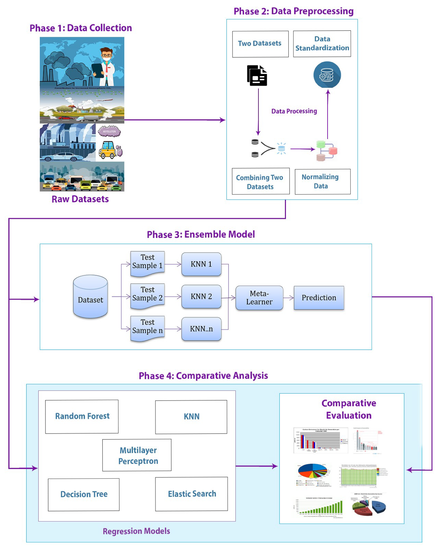
3. Methodology

This section presents the methodology for predicting traffic flow using pollution data. In phase 1 the data about pollution and intensity of traffic from the Aarhus, city website was gathered which were basically two separate datasets. In phase 2 pre-processing was done, missing values and outliers were removed. Then both datasets were merged using time stamps given in both datasets. The merged dataset was then normalized. In phase 3 different bagging and stacking ensemble model combinations were used to get the model with the least error rate which turns out to be the KNN bagging model. In phase 4 different regression models other than ensemble techniques were also used so that a comparison can be made between the resulting best ensemble technique and the regression models. Overall best performing technique with the least error rate was illustrated in methodology diagram.

3.1. Data Gathering

Collecting data and processing it is the most crucial work in any methodology and a lot of model’s performance depends on it. In this study, the dataset used was a large-scale dataset collected in real-time from city pulse Aarhus, Denmark and is publicly available. Basically, two datasets were used: data for pollution [29] and the traffic intensity dataset [30]. A lot of sensing devices were installed in the city through which information was gathered about the vehicles that were crossing by at the interval of five minutes. The information about the air pollutants is provided in the air dataset which was emitted through these vehicles that is, CO, (SO${}_2$), ozone (O${}_3$), and particulate matter (PM). The datasets traffic data for vehicle density and pollution data were of more than one year. It consists of 96,000 instances with features consisting of (O${}_3$), PM, (CO${}_2$), (SO${}_2$), (NO${}_2$), and vehicle count along with a timestamp to keep track of the time on which vehicle was arrived. As pollution data were used to predict traffic flow the data for pollution and vehicle flow was given separately. Data were collected for both pollution and vehicle flow from the Aarhus, Denmark website and combined by using the timestamps given in both datasets. In this work, data recorded in real-time was used via sensors from the dataset that was available publicly and it was an open-source dataset that contains the information about the city pulse Aarhus.

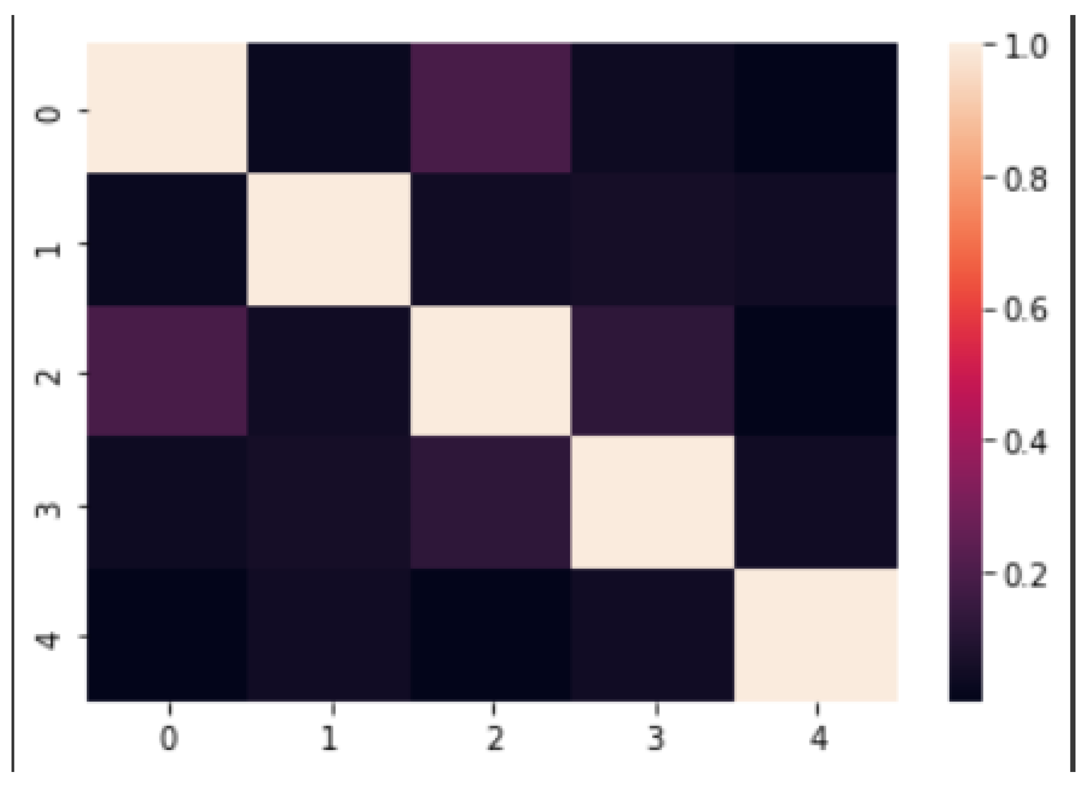
This dataset is widely used in the literature, for example, [31,32]. It is available freely on their website and can easily be downloaded and used. A zip file is provided. This file can be extracted easily and can be used accordingly. The datasets chosen for experimentations were pollution data which consists of (NO${}_2$), CO, (SO${}_2$), (O${}_3$), PM, latitude, the longitude of the location and, traffic data that consists of traffic intensity data. It consists of the data of traffic intensity between two points. A correlation matrix graph was used to check the relationship that exists between the features in the dataset as shown in Figure 2. The positive relation between the features can be seen.

In this study, no of vehicles were used according to the traffic dataset and were merged to the dataset that contains the data of pollution according to their respective time stamps. These two datasets were merged because the data were taken via sensors placed beside the roads and they were placed at the same location. Besides, how many vehicles are there is directly proportional to the emission of pollution so the more the emission of (NO${}_2$), CO and (SO${}_2$) resulting in more intensity of the traffic. The motive behind using only pollution data is to reduce the cost of the infrastructure placed to analyze the flow of traffic. Instead of focusing on the nitty-gritty, a model which can be used for general surveillance in urban cities. By using the pollution dataset the high cost can be avoided for different specific sensors and instead generalized predictions can be made reducing the number of sensors used.

A sample of the dataset is given in

Table 2. A sample of dataset.

Ozone	Particular Matter	Carbon Monoxide	Sulfure Dioxide	Nitrogen Dioxide	Time Stamp	Vehicle Count
55	38	31	51	82	8 January 2014 6:45	0
55	42	30	54	79	8 January 2014 6:50	0
50	38	29	51	82	8 January 2014 6:55	0
47	36	28	56	80	8 January 2014 7:00	0
42	41	32	54	75	8 January 2014 7:05	1
41	37	27	54	79	8 January 2014 7:10	1
37	42	24	57	81	8 January 2014 7:15	0

and also correlation matrix is given in Figure 2.

3.2. Data Pre-Processing

Processing data were performed in this phase. Processing data into the format the model will accept was the most important part to model the true relationship between input and output variables. Since the data were raw and had problems such as missing values, outliers, and so forth. Some techniques were applied to make data usable for models to take it as input and process.

Missing values do occur due to a lot of reasons for example, survey non-response, errors while entering data. To remove missing values, imputation was used by mean/median value. In order to implement this, missing values were removed by using the pandas library where at first, the column name was found out where there is a value that was missing. Afterwards index of that value was found and replaced with the mean of the values that were in the column.

Outliers are basically the data points that are not near to other data points. They are uncommon values in a dataset. Basically, outliers can be troublesome in many statistical studies because of the reason that they cause tests to miss important findings or destroy real results. These points can become the reason for the tests to miss the significant finding or it can cause them to miss the real results that are required. There is no one solution to remove outliers as it solely depends on the problem at hand. Z-scores were used to detect outliers and remove them. It indicates at what distance the data point is. It is from the mean of the whole data. When the Z-score is zero it indicates that the value is equal to the mean so that the more the Z-score is the more the value is unusual. To implement Z-score in a dataset, scipy was used. Outliers were removed using the scipy library by first calculating Z-scores and then filtering out all values which had a Z-score less than 3. Data were standardized and normalized so some algorithms such as KNN can easily process it. This is because they use distances between data points to determine their similarity.Scikit-learn library’s techniques were used for pre-processing called min-max scaler and normalization. Data normalization plays a crucial step when it comes to pre-processing data. Data normalization is responsible for the high quality of the data used for training of the model so that it remains intact and can be used as the input for ML or DL model [33]. When the features in data have different ranges, data normalization becomes very necessary. Take as an example a dataset whose traffic density values range between 0 and 50, and at the same time values ranges for (CO${}_2$) and (NO${}_2$) change from 0–4.2 and 0–300, respectively. The difference of scale can make the performance of models poor, and they may suffer due to these different ranges. Data normalization allows us to deal with these different scales in the dataset. It also helps us in reducing training time. A range of different techniques are available for data normalization such as min-max, median normalization, and Z-score decimal scaling. Well-known normalization technique, min-max normalization was used for experiments [34].

3.3. Building Regression Models by Ensemble

In this phase, an ensemble model given in Figure 3 has been developed in three steps. In the first step, data were split into various samples that have the size B and called bootstrap samples by using an initial dataset which was of size N and is done by randomly drawing out with replacement B observations. After which samples were as follows:

$$A^{n}b=a^{1}1,a^{1}2,\dots a^{1}B,\dots a^{2}1,a^{2}2,...a^{2}B.$$

(1)

In the next step, N independent weak learners were fit on each of the datasets after applying bootstrapping:

$$W^L=w^1,w^2,\dots ,w^L.$$

(2)

After fitting the N independent weak models, results of all the weak models were aggregated to get an ensemble model which has low variance which was done by the following equation:

$$A^N=1/n{\Sigma }_{i=1}^N{W}^L.$$

(3)

$A^N$ was aggregated result after ensemble.

In this research, various models were combined by using bagging ensemble techniques. The final model combined the results of various weak models to find out more accurate predictions. The process in this model works like this: splitting the dataset into various B size samples by using boostrap technique, training various weak models in parallel on different samples of the original dataset, and at the end combining the predictions made by these weak models by aggregation methods such as average to get results. The combinations of bagging ensembles used were 3 which are:

• KNN ensemble
• Random forest ensemble
• Multi-layer perceptron ensemble

Out of these three models, the KNN ensemble has the best results having the least error rate.

4. Experiments

In this section, an analysis of various experiments performed on the dataset was shown. Simple regression models were used to predict traffic intensity. After that, different ensemble models were used and a comparison was made for the results of both approaches to find out the model which performs the best of all of them.

4.1. Evaluation Metrics

To evaluate the models, well-known metrics were used. So, 4 of the most well known evaluation metrics were used which are Relative Absolute Error (RAE) [35], Mean Absolute Error (MAE) [36], R-squared (R2) [37] and RMSE (Root Mean Square Error) [38].

$$\mathrm{MAE}=1/n{\Sigma }_{i=1}^N|y_i^p-y_i^a|$$

(4)

$$\mathrm{RAE}=\sqrt{1/n{\Sigma }_i^{}{y}_i^2}$$

(5)

$$\mathrm{R}-\mathrm{squared}=\mathrm{SSR}/\mathrm{SST}$$

(6)

$$\mathrm{RMSE}=1/N\sqrt{{\Sigma }_{i=1}^N}{(x_i^A-x_i^p)}^2.$$

(7)

RAE and MAE are used to measure the errors. This is known as the difference between the predicted value and the true value. It is basically the average of all the errors calculated as predicted minus actual. R2 represents the value of the variance of the response variable learned by the regression model. The sum of squares total (SST) and the sum of squares regression (SSR) proportion is called R2. SSR shows the variation of predicted values from the mean values of the response variable. However, SST shows the variation of actual values with respect to mean values of the response variable. 1 is the value that tells us about the observed data differences and indicates that the fitted value is almost none. It is used as the best value by R-squared. The fitting of the model depends highly on this value. It indicated that if the value is higher the model fits better. RAE which is represented as a ratio, compares a mean error residual to the errors which are produced by a trivial or naive model. A good model will give a result in a ratio of less than one. The way that is used is to calculate how far the data points are from the regression line. RMSE then further calculates how far these residuals are from each other. The standard deviation of the prediction errors is known as RMSE. The RMSE is used as the standard way to evaluate the regression model and is also widely used in forecasting problems. The smaller value of RMSE is considered as the data are closest to the fitting of the model.

4.2. Experimental Settings

Colab with python 3.7.12 was used. To split the dataset, scikit-learn test train split function was used with 80/20 split along with it different predefined models from sci-kit-learn were used. Normalization and standardization using scikit-learn were performed. To read and process data numpy, scipy, and pandas were used. For visualizing data, seaborn and matplotlib were used. MAE, RMSE, R2, RAE were used for evaluating the performance of the proposed model.

4.3. Regression Models

We did a comparative analysis of various regression techniques. Data used in the experiment is open-source data from the city of Aarhus, Denmark [39]. The regression schemes used in the first category are:

4.3.1. Elastic Net

In statistics, an elastic net is basically a regularized regression method that is used linearly to combine the L1 and L2 pennants of the lasso and ridge models. The model complexity can be decreased which can be said as the number of predictors. Forward or backward selection is used in this model. By using this way, it can become unable to express anything about the variables that have been removed and had an effect on the response. By removing predictors from the technique, it can be seen as setting its coefficients to zero. It punishes them if they are too far from zero rather than making them close to zero. Continuously, it forces them to be small. In this way, the complexity of the model decreases while all variables are kept in the model.

4.3.2. K-Nearest Neighbors

The KNN algorithm supposes that alike things exist close to each other. It can be said that similar things are closer to one another. Basically, it calculates the current example distance from the data along with the query example, and, then the distance is added to the part of the ordered collection which is known as the example’s index. The sorting technique used for the ordered collection is from the smallest to largest in accessing the order through which the distances after it picks the K entries from an already sorted collection. After this, the labels of K entries are captured that were selected and if it is a regression problem returns the mean of the various K labels.

4.3.3. Multiple Linear Regression

It is called multiple regression as well. It is a statistical method. Multiple Linear Regression can use Several explanatory variables to guess the output of a response variable. The goal here is how a linear relationship can be modeled that exists between the explanatory variables that are independent and response variables that are dependent. Multiple regression is known as the extension or addition of ordinary least-squares (OLS) regression because there is more than one explanatory, or it can be said as an independent variable in MLP.

4.3.4. Multi-Layer Perceptron Regression

MLP, also known as Multilayer perceptron, is basically a feedforward ANN. MLP is also known as “vanilla” neural networks. It is only in the case when it has a single hidden layer. There are three layers on nodes through which an MLP is composed of. There should be at least three layers of a node. There can be more than three as well: an input layer, a hidden layer, and an output layer. Excluding the input nodes, all the other nodes are a neuron. The neuron uses a nonlinear activation function. It uses a technique called backpropagation in order to train the model and for training the network weights. It has multiple layers and non-linear activation functions which distinguishes MLP from a linear perceptron. It can make a difference between data that is not linearly separable.

4.3.5. Random Forest Regression

It is known as an ensemble method that can be used to perform both of the tasks related to regression as well as classification. Multiple decision trees are used by it. It also uses different methods called Bootstrap and Aggregation, also known as bagging, in order to perform the regression and classification tasks. It combines multiple decision trees in guessing the final output which is the fundamental idea behind using this technique. It does not rely on individual decision trees. By using the random forest feature row sampling can be performed randomly on the data. For every model, sample datasets are formed. This method is also called bootstrapping. While performing the regression tasks the average prediction or the mean of the individual trees is returned.

4.3.6. Decision Tree

Regression models are constructed by using the decision trees. They are constructed in the shape of a tree structure. A dataset is broken into subsets that are smaller. As this process is continued an associated decision tree is constructed. The tree is constructed incrementally. As a result, a tree is found that consists of the decision nodes and the leaf nodes. There are two or more branches for a decision node, each of the branches illustrates values for the attribute that are tested. A decision is constituted by the leaf nodes on the numerical target. The node that is on the decision tree is the node that corresponds to the best predictor. It is called the root node. Decision trees can be used in both regression and classification tasks.

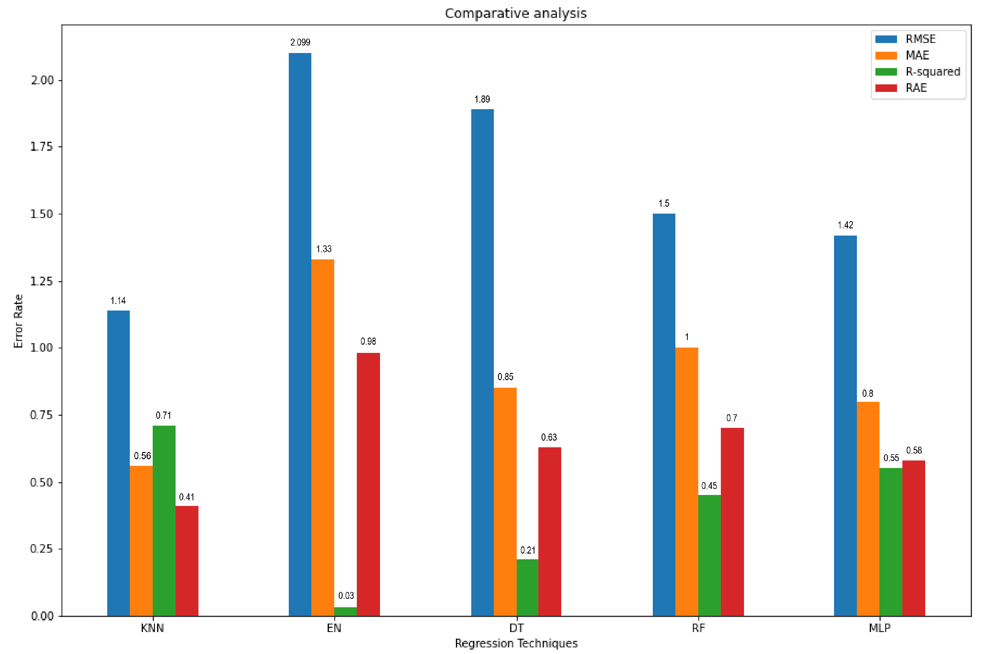
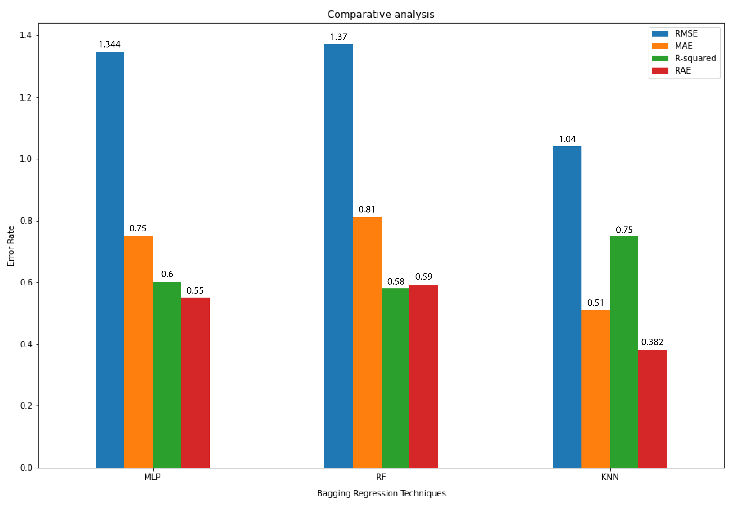
4.4. The Comparative Analysis of Various Regression Techniques

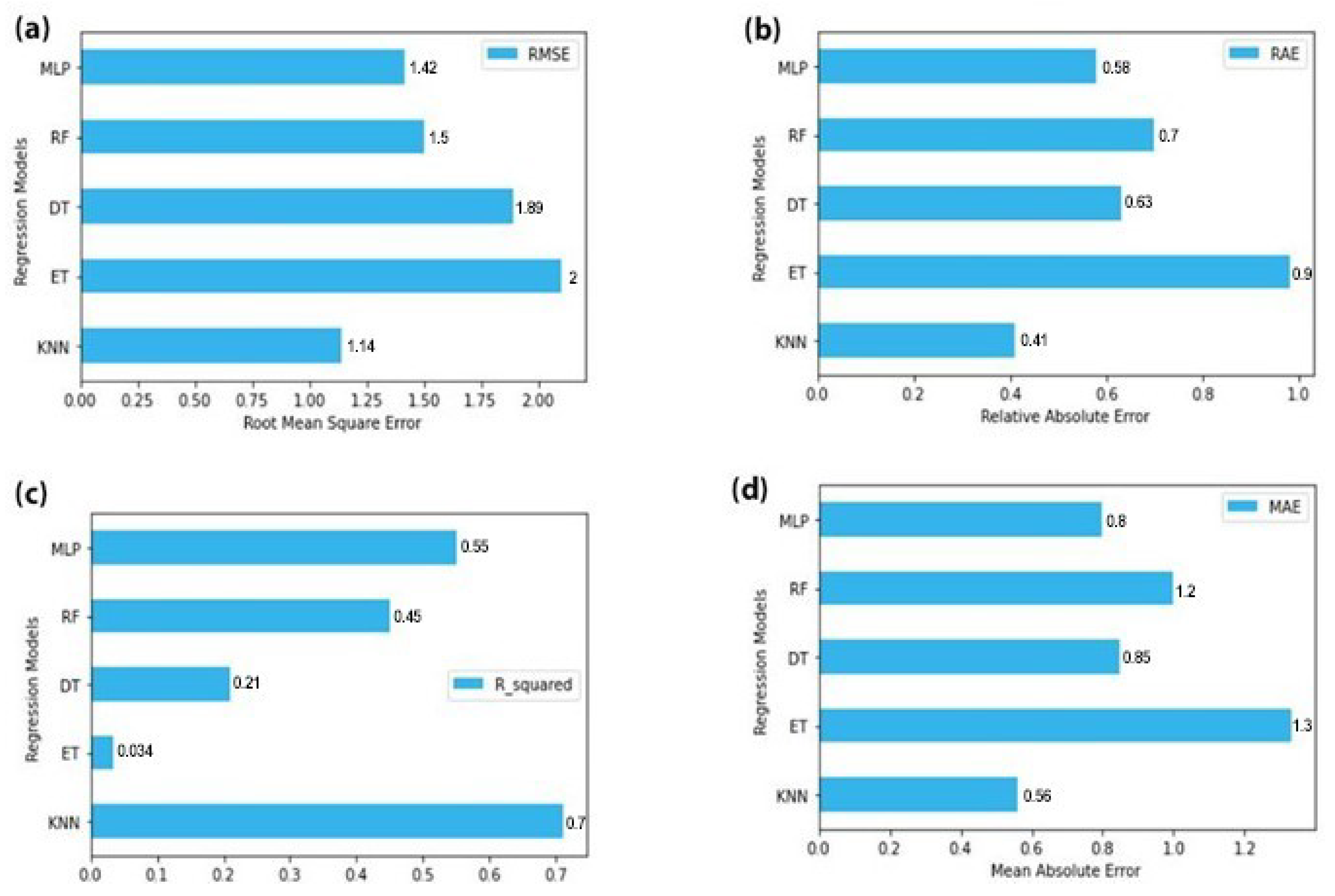
Each of the regression models used in the experiment is compared and contrasted in this section. These regression models are used to conclude which model is providing the best performance on traffic forecasting. In this part, the performance of each model concerning others is shown in predicting traffic flow that is, number of vehicles. Various techniques were used in these models such as MAE, RSME, RAE, and R2. The RSME values are shown in Figure 4a. These are the RSME values of all the regression models that are used in these experiments. RSME is being used as the standard deviation for the prediction models. In order to calculate how far the data points are from the regression line, the residuals are used. RMSE calculates how far from each other these residuals are. For forecasting, RMSE is commonly used and a standard way to evaluate regression models. The smaller value of RSME indicates that the data points are closer to being fit by the model. In Figure 4a the x-axis is labeled as RMSE value. The regression technique is used as the label for the y-axis. Under the provided scenario KNN gave us the best results for the expected prediction.

Figure 4d is showing the MAE values for the regression models. MAE is the amount of error in your measurements. It is known as the difference between two values that are the predicted value and the true value. This is basically the average of all the errors calculated as predicted minus actual. In Figure 4d X-axis was labeled as MAE value and the y-axis as regression models used. The lesser the value of MAE the more accurate model is. Under the provided scenario the values of MLP and KNN are the lowest.

In Figure 4c values of R2 are shown for the models. R2 is used to represent the value of the variance of the response variable that is learned by the regression model. 1 is the best value for R2. It tells us the differences that are in the data that is observed and values that are fitted is almost none. In order to make the model better fit, a high value of R2 is required. KNN has given us the highest value for R2.

Figure 4b is showing the RAE, which is represented as a ratio, this ratio compares to a mean error (residual) to the errors which are the result of a trivial or naive model. A good model will give a result in a ratio of less than one. In Figure 4b the x-axis is given the label as RAE values and the y-axis is labeled as models used. As can be seen from the graph KNN and MLP are giving the lowest values for RAE. A complete chart showing RMSE, MAE, R2 and RAE is given in Figure 5.

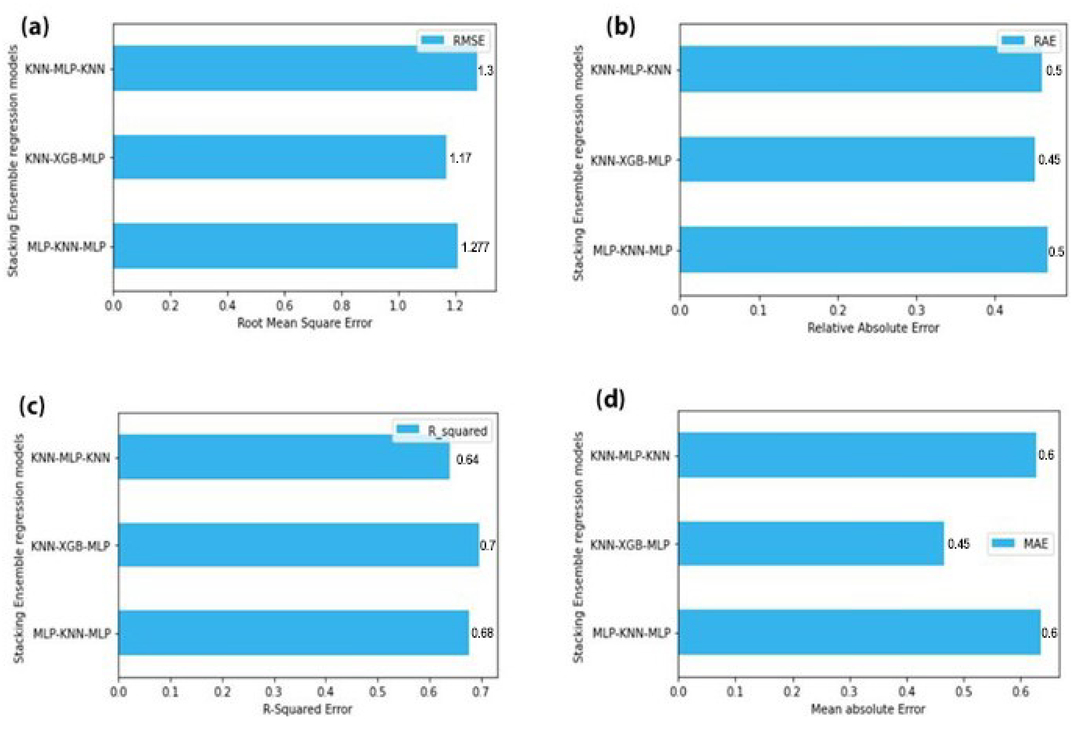
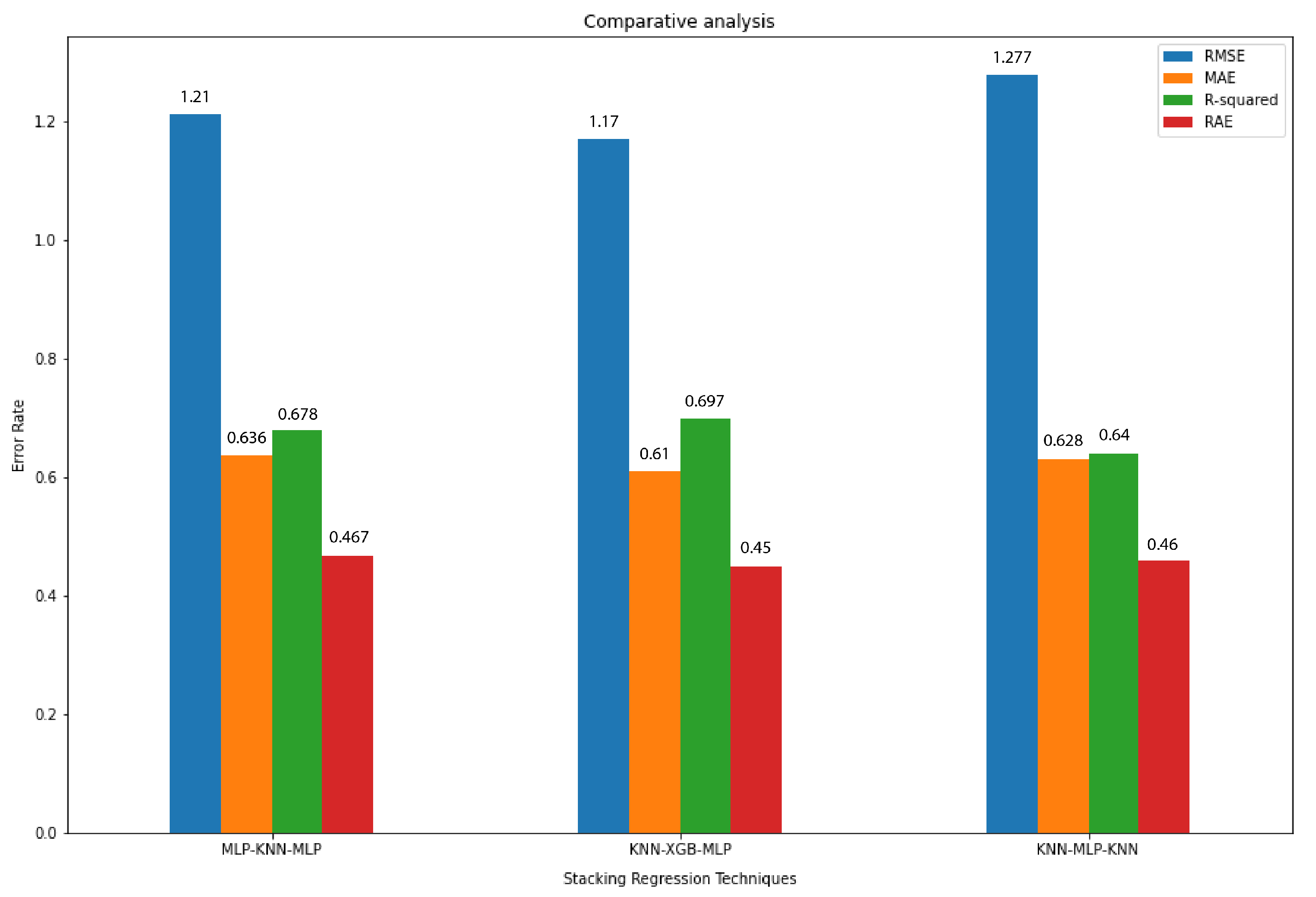
4.5. Comparison of Different Ensemble Models

The goal of this comparison is to evaluate the different ensemble combinations used and dig the best-performing one out of all those. The model with the best predictions on pollution data.

4.5.1. Stacking Ensemble

Stacking is an ensemble technique in which more than one different weak models/learners are combined. It is done by getting the output as predictions by training a meta-model. The output predictions from this model are based upon predictions that were returned by all these weak models. Two things are defined to construct a stacking model: firstly, the N learners that are required to fit, and secondly: the last model called meta-model which will combine them. Following are the steps stacking ensemble model follows:

• It splits the data used for training into two folds
• After splitting the data, it chooses N weak learners and fit these models to the data of the first fold
• After done with fitting the models it makes predictions for each N weak learner on observations in the second fold of the training data.
• Finally, it fits the meta-model to the second fold of training data, by using predictions as features made by weak learners

The results of stacking ensemble are given in Figure 6 and Figure 7.

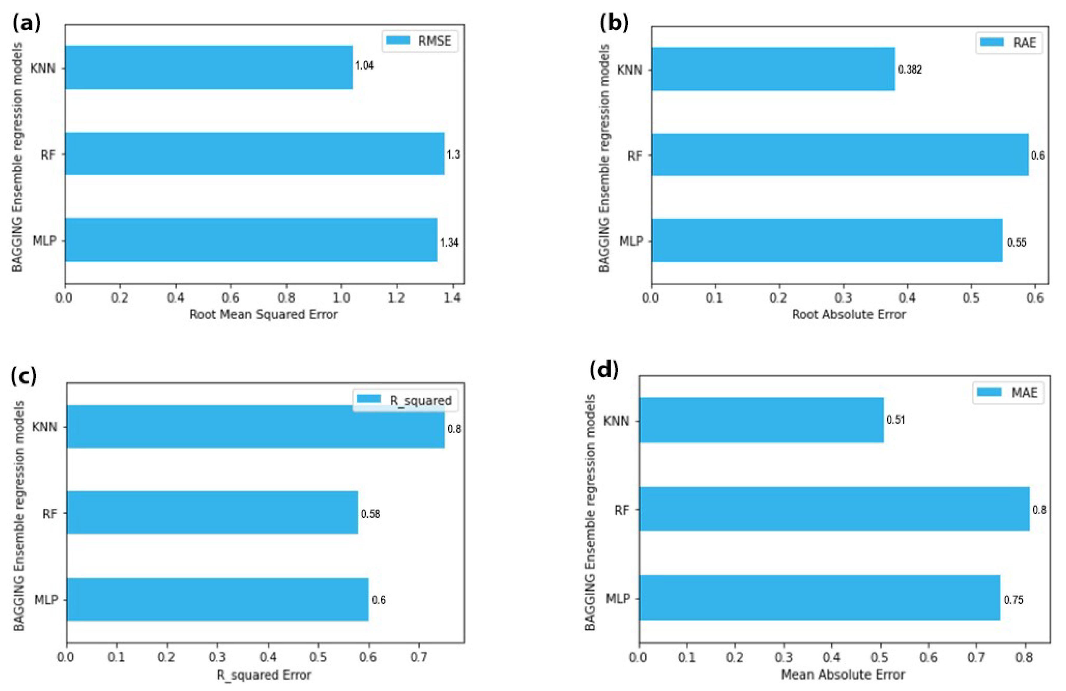
4.5.2. Bagging Ensemble

In this technique, several models of the same type were fit and then an average of those predictions was taken. First, popular stacking ensemble techniques were used and different combinations of models were stacked and turns out the stack of KNN, XGBoost, and MLP is giving the best results. Then bagging ensemble was used and different ensemble models were tried via bagging and turns out bagging KNN gives the best results as shown in Figure 8 and Figure 9.

According to the results, the RMSE value for the KNN bagging model is 1.12 which is the lowest amongst all the other values. The value of MAE is 0.55 for the best ensemble model. The value of RAE for best-performing model is 0.4 which is again the lowest amongst all. Finally, the R2 value for the model is the highest of all. The reason was that boosting ignores overfitting and variance issues in models but the ensemble technique called bagging helps to deal with high variance and overfitting. It provides an environment in which N models of the same size and algorithm can be used to deal with variance. When bagging samples in data there are many observations that overlap, so by merging more than one learner of the same algorithm prevents high variance.

4.6. KNN Bagging Hyperparameters

• Neighbours: The number of neighbors values used was 3.
• Estimators: It is the number of base learners used which in case was 10.
• Random State: The value of the random state used was 0 which can be used to reproduce results easily.

4.7. Experiment Results

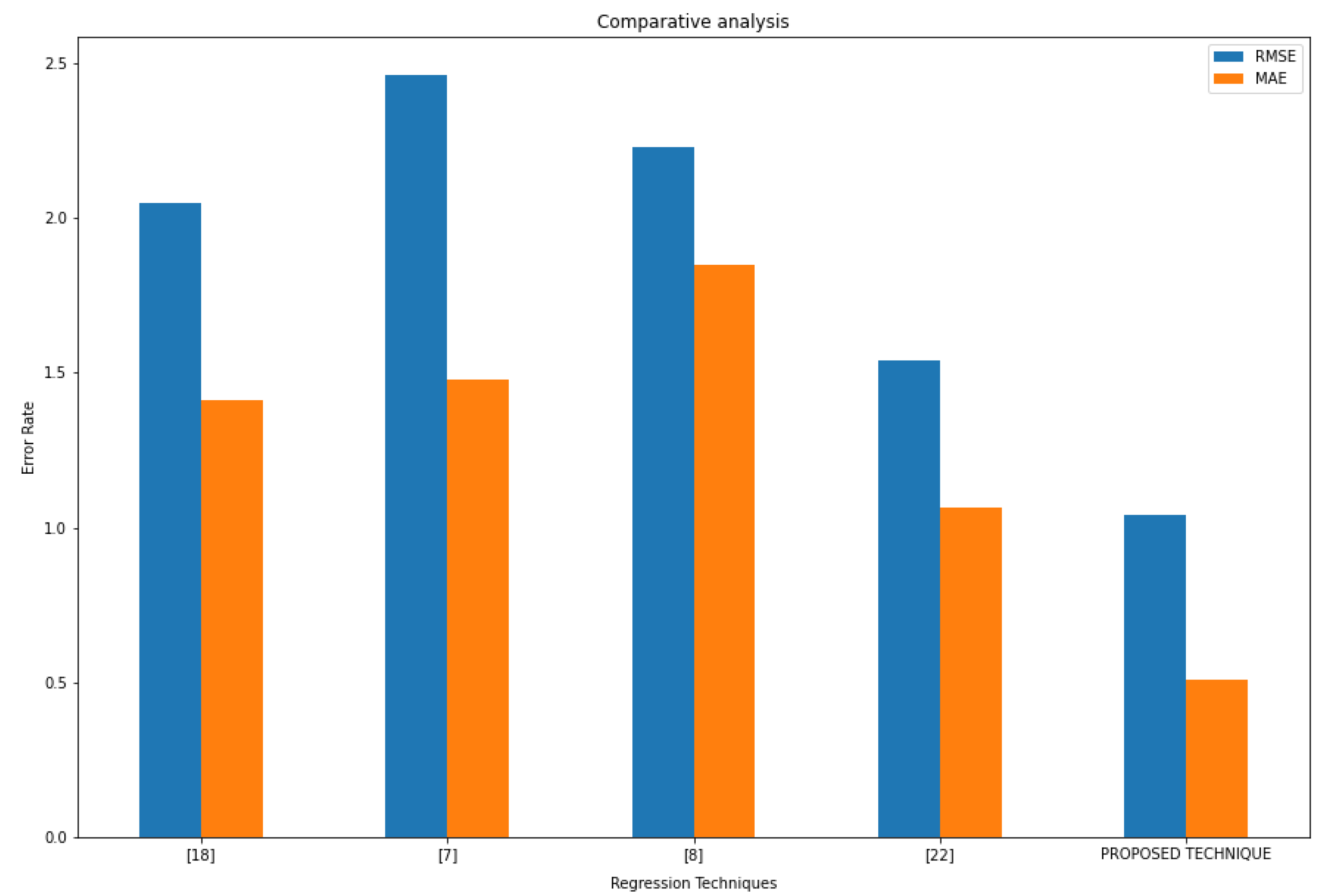
In Figure 10, results of the model were compared with different other baseline models by using two widely used error metrics for measuring the performance of regression models. RMSE and MAE values were interpreted as the error rate of a model which is the difference between actual and predicted value by model. If RMSE and MAE values are high, it means models have high error but if it is low then the model is considered to have learned better. As can be seen in Figure 10. The model has the least error among all baseline models, which means the model has learned significantly better than other models. This study is also compared to the base paper [21]. The experiments showed that the error rate was improved by more than 30% using a bagging ensemble as opposed to boosting ensemble used in [21]. The two studies are similar in the way that both are using the same dataset and problem. The first step of data pre-processing is generally the same in almost all ML tasks. In both studies few ML models such as ANN, Decision Tree are the same. The KNN and Elastic Net models were used while [21] have not used these techniques. The results of the base paper for this study were also presented in Figure 10 when the performance of the proposed scheme was compared with other studies.

5. Discussion

In this section issues with the bagging ensemble were discussed, comparison of the model’s performance on varying dataset sizes. The model’s threats to validity are also discussed.

5.1. Issues in Bagging

As can be seen before one of the best performing models is KNN based bagging. So, if the model is providing the best results for traffic predictions why this kind of approach is not used for another related task as well. There are some issues pertaining to bagging which are the following:

• It increases the storage space and computation time because of the reason that vast number of base classifiers are used [40]
• Bagging can be the reason for losing the model’s interpretability and can have a lot of bias if there is any issue in following the standard procedure of applying bagging. It may result in model underfitting data [41]

5.2. Model Comparison on Different Dataset Sizes

The best model, which is bagging KNN, was trained and tested on a dataset with 96 k instances. Then to check that the model is doing well even if it is given a dataset with fewer instances the dataset was randomized and then 20 k instances were picked and models were trained on it. Then model results were tested which are given separately in

Table 3. Comparison of different bagging ensemble combinations used.

Dataset	Ensemble Regression Techniques	RMSE	MAE	R-Squared	RAE
Dataset with 96 k Instances	MLP	1.344	0.75	0.6030	0.55
	RF	1.37	0.81	0.59	0.59
	KNN	1.04	0.51	0.382	0.382
Dataset with 20 k Instances	MLP	1.4	0.8	0.7	0.52
	RF	1.4	0.9	0.62	0.56
	KNN	1.1	0.54	0.4	0.4

. It can be seen that the results are nearly the same as they were on a big dataset. The minor difference seen is caused by the fact that the more data, the more patterns the model will learn and in turn does better.

5.3. Threat to Validity

Currently, Aarhus City data were used only. So, as electric cars are becoming widespread which will have a huge impact on the amount of pollution being generated around big cities. It is a great factor that could be impacting predictions in long term, however, the replacement of electric vehicles with old vehicles will not be immediate. This delay in adoption could be the catalyst for the model to learn new patterns in the meantime. Because air pollution is increasing the adoption of electric vehicles in the world. Take an example of the nation’s electric mobility missing which is expecting the sale of electric vehicles of around seven million annually from 2020 and onwards [42]. As it is obvious that a longer timeframe will be needed for the world to completely replace/eliminate conventional vehicles, their replacement could be a threat to the approach proposed, because of the reason that it depends partially on the emission of pollution from these vehicles.

6. Conclusions and Future Work

For smart cities traffic flow prediction is the most crucial task. Precise traffic forecasting can help drivers manage their trips effectively. To accurately predict traffic flow, this study initially combined pollution and traffic datasets of Aarhus, Germany. Then different conventional ML approaches were used on the dataset to find out the most accurate approach among them. KNN had the least MAE and RMSE values among them. After observing the results of conventional approaches, the bagging and stacking ensemble was used to improve the MAE and RMSE values. Bootstrapping was used with replacement to split the dataset into samples. The samples were fed into the different number of homogeneous models and their result was aggregated to form a strong bagging ensemble model. KNN bagging ensemble model proved to be the most accurate among all bagging and stacking ensemble combinations. One reason for KNN being more accurate is that the dataset is non-linear in nature and KNN performs well at non-linear data, but it can underfit if the number of nearest neighbors K is too small and can get overfit if it is too large. Experimental results suggest that the proposed bagging ensemble scheme reduced the error rate by 30% over previous studies which used boosting to predict traffic flow in smart cities. The dataset had a lot of outliers which caused boosting ensemble models to overfit. The experiments suggest that the proposed bagging ensemble scheme reduced the effect of overfitting and resulted in an improved error rate. It decreased the error by 12% over KNN and stacking ensemble models which were used in our study. There are some issues related to bagging. Firstly, it increases the storage space and computation time. Secondly, because of the reason, that a vast number of base classifiers were used, bagging can be the reason for losing the model’s interpretability and can result in biasness if there is any issue in following the standard procedure of applying bagging. It may result in model underfitting data. Dataset of different areas of Aarhus, Germany was used so the model will slightly suffer in other areas of the world where seasons and traffic patterns are different.

In future, the effects of different seasons such as summer and winter will be investigated. The patterns of traffic vary as people in European countries go on vacations and leave cities in August. The future study will also focus on finding contributions in air pollution by road traffic, home, and different types of equipment. In different cities, the correlation between traffic and pollution data may differ. Satellite measurements for traffic can be considered in combination with ground sensor values to understand if they both can be used in combination to predict traffic flow. Moreover, the data of more cities of the world will be included to check the robustness and other performance parameters.

References

- Jonathan Levy, K.V. Emissions from Traffic Congestion May Shorten Lives. Available online: https://www.hsph.harvard.edu/news/hsph-in-the-news/air-pollution-traffic-levy-von-stackelberg/ (accessed on 23 November 2021).
- Badger, E. How Traffic Congestion Affects Economic Growth. Available online: https://www.bloomberg.com/news/articles/2013-10-22/how-traffic-congestion-affects-economic-growth (accessed on 23 November 2021).
- UKELA (UK Environmental Law Association). Road Traffic. Available online: http://www.environmentlaw.org.uk/rte.asp?id=38 (accessed on 23 November 2021).
- World Health Organization. Air Pollution and Climate Change. Available online: https://www.who.int/health-topics/air-pollution (accessed on 23 November 2021).
- Chen, V.H.; Xie, Q.; Wang, R.; Simunek, M.; Smutny, Z.; Alobaidi, M.; Badri, R.M.; Salman, M.M. Evaluating the Negative Impact of Traffic Congestion on Air Pollution at Signalized Intersection. In Proceedings of the IOP Conference Series: Materials Science and Engineering, 4th International Conference on Buildings, Construction and Environmental Engineering, Istanbul, Turkey, 7–9 October 2019; Volume 737. [Google Scholar] [CrossRef]
- Krishan, M.; Jha, S.; Das, J.; Singh, A.; Goyal, M.K.; Sekar, C. Air quality modelling using long short-term memory (LSTM) over NCT-Delhi, India. Air Qual. Atmos. Health 2019, 12, 899–908. [Google Scholar] [CrossRef]
- Bogaerts, T.; Masegosa, A.D.; Angarita-Zapata, J.S.; Onieva, E.; Hellinckx, P. A graph CNN-LSTM neural network for short and long-term traffic forecasting based on trajectory data. Transp. Res. Part C Emerg. Technol. 2020, 112, 62–77. [Google Scholar] [CrossRef]
- Zhang, W.; Yu, Y.; Qi, Y.; Shu, F.; Wang, Y. Short-term traffic flow prediction based on spatio-temporal analysis and CNN deep learning. Transp. A Transp. Sci. 2019, 15, 1688–1711. [Google Scholar] [CrossRef]
- Ma, Y.; Zhang, Z.; Ihler, A. Multi-Lane Short-Term Traffic Forecasting with Convolutional LSTM Network. IEEE Access 2020, 8, 34629–34643. [Google Scholar] [CrossRef]
- Cui, Z.; Ke, R.; Pu, Z.; Wang, Y. Stacked bidirectional and unidirectional LSTM recurrent neural network for forecasting network-wide traffic state with missing values. Transp. Res. Part C Emerg. Technol. 2020, 118, 102674. [Google Scholar] [CrossRef]
- Zhan, X.; Zhang, S.; Szeto, W.Y.; Chen, X. Multi-step-ahead traffic speed forecasting using multi-output gradient boosting regression tree. J. Intell. Transp. Syst. 2019, 24, 125–141. [Google Scholar] [CrossRef]
- Guo, J.; Liu, Y.; Yang, Q.; Wang, Y.; Fang, S. GPS-based citywide traffic congestion forecasting using CNN-RNN and C3D hybrid model. Transp. A Transp. Sci. 2020, 17, 190–211. [Google Scholar] [CrossRef]
- Cheng, S.; Lu, F.; Peng, P. Short-term traffic forecasting by mining the non-stationarity of spatiotemporal patterns. IEEE Trans. Intell. Transp. Syst. 2021, 22, 6365–6383. [Google Scholar] [CrossRef]
- Bai, J.; Zhu, J.; Song, Y.; Zhao, L.; Hou, Z.; Du, R.; Li, H. A3T-GCN: Attention Temporal Graph Convolutional Network for Traffic Forecasting. ISPRS Int. J. Geo-Inf. 2021, 10, 485. [Google Scholar] [CrossRef]
- Barua, S. A Naïve Bayes Classifier Approach to Incorporate Weather to Predict Congestion at Intersections. World Acad. J. Eng. Sci. 2020, 7, 72–76. [Google Scholar]
- Cheng, S.; Lu, F.; Peng, P.; Wu, S. Short-term traffic forecasting: An adaptive ST-KNN model that considers spatial heterogeneity. Comput. Environ. Urban Syst. 2018, 71, 186–198. [Google Scholar] [CrossRef]
- Xu, D.; Wang, Y.; Peng, P.; Beilun, S.; Deng, Z.; Guo, H. Real-time road traffic state prediction based on kernel-KNN. Transp. A Transp. Sci. 2018, 16, 104–118. [Google Scholar] [CrossRef]
- Voort, M.V.D.; Dougherty, M.; Watson, S. Combining kohonen maps with arima time series models to forecast traffic flow. Transp. Res. Part C Emerg. Technol. 1996, 4, 307–318. [Google Scholar] [CrossRef] [Green Version]
- Kim, H.W.; Lee, J.H.; Choi, Y.H.; Chung, Y.U.; Lee, H. Dynamic bandwidth provisioning using ARIMA-based traffic forecasting for Mobile WiMAX. Comput. Commun. 2011, 34, 99–106. [Google Scholar] [CrossRef]
- Li, Z.; Zheng, Z.; Washington, S. Short-Term Traffic Flow Forecasting: A Component-Wise Gradient Boosting Approach with Hierarchical Reconciliation. IEEE Trans. Intell. Transp. Syst. 2020, 21, 5060–5072. [Google Scholar] [CrossRef]
- Shahid, N.; Shah, M.A.; Khan, A.; Maple, C.; Jeon, G. Towards greener smart cities and road traffic forecasting using air pollution data. Sustain. Cities Soc. 2021, 72, 103062. [Google Scholar] [CrossRef]
- Zhou, T.; Han, G.; Xu, X.; Lin, Z.; Han, C.; Huang, Y.; Qin, J. δ-agree AdaBoost stacked autoencoder for short-term traffic flow forecasting. Neurocomputing 2017, 247, 31–38. [Google Scholar] [CrossRef]
- Zhang, C.; Yu, J.J.; Liu, Y. Spatial-Temporal Graph Attention Networks: A Deep Learning Approach for Traffic Forecasting. IEEE Access 2019, 7, 166246–166256. [Google Scholar] [CrossRef]
- Lu, H.; Huang, D.; Song, Y.; Jiang, D.; Zhou, T.; Qin, J. ST-TrafficNet: A Spatial-Temporal Deep Learning Network for Traffic Forecasting. Electronics 2020, 9, 1474. [Google Scholar] [CrossRef]
- Kumar, D.T.S. Video based Traffic Forecasting using Convolution Neural Network Model and Transfer Learning Techniques. J. Innov. Image Process. 2020, 2, 128–134. [Google Scholar] [CrossRef]
- Ketabi, R.; Al-Qathrady, M.; Alipour, B.; Helmy, A. Vehicular traffic density forecasting through the eyes of traffic cameras; a spatio-temporal machine learning study. In Proceedings of the 9th ACM Symposium on Design and Analysis of Intelligent Vehicular Networks and Applications, Miami Beach, FL, USA, 25–29 November 2019; pp. 81–88. [Google Scholar] [CrossRef] [Green Version]
- Sun, S. Traffic flow forecasting based on multitask ensemble learning. In Proceedings of the First ACM/SIGEVO Summit on Genetic and Evolutionary Computation, Shanghai, China, 12–14 June 2009; pp. 961–964. [Google Scholar] [CrossRef]
- Moretti, F.; Pizzuti, S.; Panzieri, S.; Annunziato, M. Urban traffic flow forecasting through statistical and neural network bagging ensemble hybrid modeling. Neurocomputing 2015, 167, 3–7. [Google Scholar] [CrossRef]
- CityPulse Dataset Collection. Pollution Dataset. Available online: http://iot.ee.surrey.ac.uk:8080/datasets.html#pollution (accessed on 23 November 2021).
- CityPulse Dataset Collection. Traffic Dataset. Available online: http://iot.ee.surrey.ac.uk:8080/datasets.html#traffic (accessed on 23 November 2021).
- Zenkert, J.; Dornhofer, M.; Weber, C.; Ngoukam, C.; Fathi, M. Big data analytics in smart mobility: Modeling and analysis of the Aarhus smart city dataset. In Proceedings of the 2018 IEEE Industrial Cyber-Physical Systems (ICPS), St. Petersburg, Russia, 15–18 May 2018; pp. 363–368. [Google Scholar] [CrossRef]
- Honarvar, A.R.; Sami, A. Multi-source dataset for urban computing in a Smart City. Data Brief 2019, 22, 222–226. [Google Scholar] [CrossRef] [PubMed]
- Nayak, S.C.; Misra, B.B.; Behera, H.S. Impact of data normalization on stock index forecasting. Int. J. Comput. Inf. Syst. Ind. Manag. Appl. 2014, 6, 257–269. [Google Scholar]
- Gajera, V.; Gupta, R. An effective multi-objective task scheduling algorithm using min-max normalization in cloud computing. In Proceedings of the 2016 2nd International Conference on Applied and Theoretical Computing and Communication Technology (iCATccT), Bangalore, India, 21–23 July 2016; pp. 812–816. [Google Scholar]
- Collopy, F.; Armstrong, J.S. Another Error Measure for Selection of the Best Forecasting Method: The Unbiased Absolute Percentage Error; University of Pennsylvania: Philadelphia, PA, USA, 1994. [Google Scholar]
- Tan, M.C.; Wong, S.C.; Tunku, U.; Rahman, A.; Zhang, P.; Wong, S.C.; Xu, J.M.; Guan, Z.R. An aggregation approach to short-term traffic flow prediction. IEEE Trans. Intell. Transp. Syst. 2009, 10, 60–69. [Google Scholar] [CrossRef]
- Hochreiter, S.; Schmidhuber, J. Long Short-Term Memory. Neural Comput. 1997, 9, 1735–1780. [Google Scholar] [CrossRef]
- Castro-Neto, M.; Jeong, Y.; Jeong, M. Online-SVR for Short-Term Traffic Flow Prediction under Typical and Atypical Traffic Conditions. In Expert Systems with Applications, Part 2; Elsevier: Amsterdam, The Netherlands, 2019; Volume 36, pp. 6164–6173. [Google Scholar]
- CityPulse Smart City Datasets. Available online: http://iot.ee.surrey.ac.uk:8080/ (accessed on 23 November 2021).
- Baba, N.; Makhtar, M.; Fadzli, S. Current issues in ensemble methods and its applications. J. Theor. Appl. Inf. Technol. 2015, 81, 266–276. [Google Scholar]
- Fumera, G.; Roli, F.; Serrau, A. A theoretical analysis of bagging as a linear combination of classifiers. IEEE Trans. Pattern Anal. Mach. Intell. 2008, 30, 1293–1299. [Google Scholar] [CrossRef]
- Nimesh, V.; Sharma, D.; Reddy, V.M.; Goswami, A.K. Implication viability assessment of shift to electric vehicles for present power generation scenario of India. Energy 2020, 195, 116976. [Google Scholar] [CrossRef]