Article

Contributions of Wetland Plants on Metal Accumulation in Sediment

by
Marelé A. Nel
1,2,*,
Gletwyn Rubidge
3,
Janine B. Adams
1 and
Lucienne R. D. Human
1,2,*
1
Department of Botany, DSI/NRF Research: Shallow Water Ecosystems, South Campus, Nelson Mandela University, Summerstrand, Port Elizabeth 6031, South Africa
2
South African Environmental Observation Network (SAEON) Elwandle Coastal Node, Ocean Sciences Campus, Nelson Mandela University, 4 Gomery Avenue, Summerstrand, Port Elizabeth 6031, South Africa
3
Department of Chemistry, Summerstrand North Campus, Nelson Mandela University, Port Elizabeth 6031, South Africa
*
Authors to whom correspondence should be addressed.
Sustainability 2022, 14(6), 3679; https://doi.org/10.3390/su14063679
Submission received: 31 January 2022 / Revised: 11 March 2022 / Accepted: 14 March 2022 / Published: 21 March 2022
(This article belongs to the Special Issue Aquatic Plants as Bioindicators of Trace Metal Pollution)

Abstract

:
Wetlands, and especially salt marshes, are well-known sinks of metals, which limit toxic amounts of metals from entering the food chain. This study investigated metal concentrations (Cr, Cu, Fe, Mn, Ni, Pb, Zn) in a highly urbanised estuary, and compared vegetated rhizosediment (Salicornia tegetaria, Spartina maritima, and Zostera capensis) with bare sediment, in a depositional and non-depositional site, in the intertidal zone of the Swartkops Estuary. The samples were collected at two sites along the middle and lower reaches of the estuary and analysed using a Total X-ray Fluorescence (TXRF) spectrometer. It was found that the rhizosediment contained more metals and that metal concentrations in the sediment decreased as follows: S. tegetaria > S. maritima > Z. capensis > bare sediment. Although metal accumulation was similar in bare sediment for the depositional (Site B) and the non-depositional site (Site A), the rhizosediment displayed higher metal accumulation in the depositional site (Site B). However, regardless of site-specific depositional tendencies, rhizosediment displayed higher metal accumulation than bare sediment. These results indicate that vegetated sites and vegetated depositional sites should be the focus of monitoring metals in estuaries around the world.

1. Introduction

Estuarine wetlands are primary producers that receive high natural and anthropogenic metal loads, which makes them ideal candidates to monitor ecosystem health in an estuary. Estuaries are often developed and utilised for effluent release of urban and industrial wastewater, tourism, fishing, and bait collecting. The loss of ecosystem health can lead to the loss of ecosystem function, which makes these activities unsafe [1]. Wetlands play an important role in the biogeochemistry of metals in an estuary, by acting as a buffer and sink to metals, they can prevent toxic levels from entering the food chain [2,3]. The human population is disproportionally distributed to favour coastal areas, which further puts pressure on estuarine habitats, through the release of effluent [4]. It was wrongly assumed that the toxic effects of pollutants in effluent would be nullified by the dilution of estuarine and marine water [5]. Instead, the estuarine habitats acted as filters of metal contaminants, capturing metals into their tissues and in the rhizosediment [6]. Metal pollutants are generally accumulated into the sediment close to the source, but the hydrodynamics of the estuarine environment can redistribute the metal-rich particles throughout the estuary [7]. The natural hydrodynamics of an estuary can be changed by man-made structures, creating areas that trap metal-enriched particles flowing downstream.
The extent of metal accumulation in estuarine sediment will depend on the physico-chemical characteristics of the sediment, as well as the biological elements in sediment. Estuarine salt marshes are periodically flooded due to river currents and tidal action. They retain large quantities of suspended particles (natural and anthropogenic of origin), due to the elevated topography and the vegetation structure trapping particles. The salt marshes act as a trap for many contaminants and are important sinks for metal pollutants [2,8]. Once the metals are accumulated and distributed the sediment and the plants of these habitats capture the metals by assimilating them in their biomass [9]. However, salt marsh plants often accumulate metals in their roots, keeping toxic concentrations of metals away from other parts of the ecosystem [6,9,10]. Toxic concentrations of the metals are accumulated away from the sensitive photosynthetic apparatus, allowing the plant to tolerate high nutrient loads, and promoting cycling of metals between the roots and sediment [11]. Strategies for metal tolerance are not uncommon in halophytes, because of the susceptibility of the area to high loads of nutrients [3,12]. Therefore, wetland plants (and habitats) are often used for biomonitoring, to indicate whether an environment has reached toxic levels.
Metal accumulation in sediment is dependent on the chemical and physical attributes of the sediment environment [13]. Vegetation can change the sediment environment in between their roots (i.e., in the rhizosediment) in various ways. Different inundation periods driven by higher surface elevation, coupled with the reduced wave energy from vegetated structures, promotes the deposition of enriched particles during tidal fluctuations [14]. Therefore, vegetation can increase the metal accumulation capacity of sediment by promoting smaller sediment grain sizes and producing and promoting the decomposition of organic matter. Radial Oxygen Loss (ROL) is an adaptation of macrophytes to saturated (waterlogged) conditions and results in the oxygenation of the rhizosphere, which changes the redox environment of the sediment [15,16,17]. The sediment environment plays a major role in forming either mobile (bioavailable) or immobile metal species [18,19,20]—grain size, pH, redox organic content, salinity, and Fe and Mn oxides can all influence the metal accumulation capacity of sediment [21]. Metals accumulated into the bottom sediment is in flux with the overlying water column, which indicates that a change in conditions can trigger the dissolution of metals into the water column [22].
The aim of this study was to investigate metal concentrations between dominant salt marsh (Spartina maritima and Salicornia tegetaria) and seagrass (Zostera capensis) rhizosediment, and bare sediment, at the same sites in the Swartkops Estuary. Metal concentrations in rhizosediment and bare sediment within a depositional and non-depositional site, in the middle and lower reaches of the estuary, were compared. The unvegetated (bare) mudflats were near the vegetated areas and would receive similar metal load and have similar hydrodynamic influences. Assessing whether metal concentrations in bare sediment are comparable to concentrations in rhizosediment, assists in promoting vulnerable salt marsh and seagrass habitats for conservation. This study theorises from past research in other estuaries that metal accumulation will be significantly higher in the rhizosediment compared to the bare sediment. The results will remind future researchers to approach metal studies in vegetated areas differently from bare areas.

2. Materials and Methods
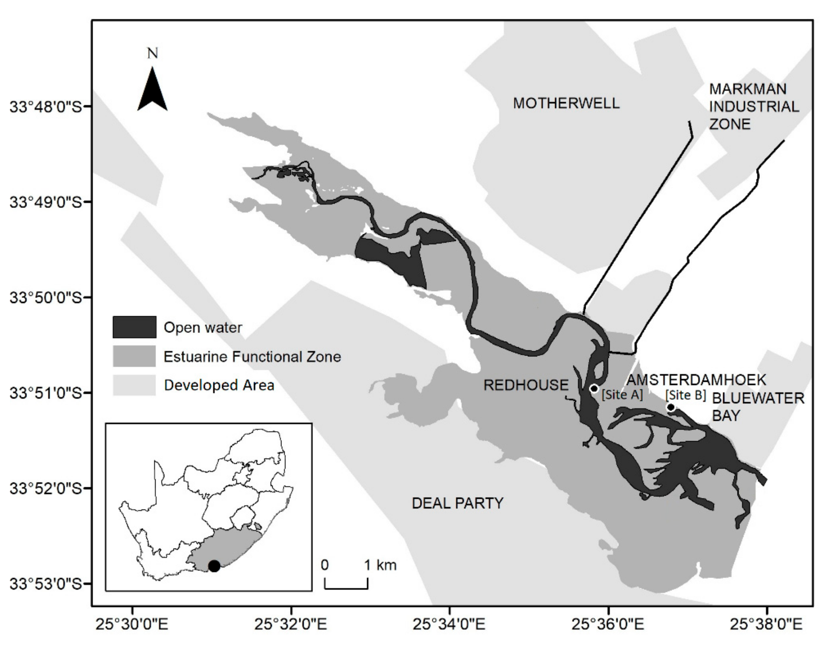
2.1. Study Site

Sampling occurred at two different sites in the Swartkops Estuary, a predominantly open estuary located on the warm-temperate south-east coast of South Africa (Figure 1) [23]. The sites were located in the intertidal area of the middle and lower reaches of the estuary. Site A (Markman Canal) was located close to an industrial point source, while Site B (Tippers’ Creek) was in a highly urbanised creek (Figure 1). The freshwater inflow into the estuary is restricted by damming and tributaries that reduces freshwater inflow by 5% [24]. It is well mixed and exhibits highly stratified waters only during a high flood event. The salt marshes cover an area of approximately 547.4 ha and are dominated by S. maritima in the lower reaches [23]. Salicornia sp. are found higher up the tidal gradient of the saltmarsh, while seagrass beds consisting of Z. capensis are found along the subtidal-intertidal fringe [25]. Swartkops Estuary contains some of the largest Z. capensis beds [23]. These habitats are essential for nutrient cycling, fish nurseries, and aquatic habitat. The middle and lower reaches of the estuary is surrounded by rural, urban, and industrial zones, which contribute to effluent released into the estuary. The major industrial activities in the vicinity include saltpans, sewage works, sand/clay mining, brickworks, a power station, motor industry, wool industry, tanneries, extraction/beneficiation processes, aquaculture, railway yards, depots, and some agriculture [24,26]. The estuary is therefore subjected to high anthropogenic pressure, with the potential to introduce metal contaminants.

2.2. Sampling

Once-off sampling was carried out in winter 2019, during spring low tides. Plants and their accompanying sediment samples were collected at each site in replicates of five. Sediment samples were collected along the shore of the estuary within homogenous patches of Z. capensis, S. maritima, and S. tegetaria, and adjacent unvegetated mudflats. The plants were randomly selected along a vertical line so that the three species were within an intertidal range from each other. Sediment from the surface (0–10 cm) of the rhizosphere was collected and contained within 50 mL plastic jars with a screw cap. A PVC corer (radius = 5.6 cm) was used to remove whole plant biomass from the selected plants, being careful to keep the roots intact (depth = ca. 20 cm). The jars were then contained within sealable ziplock packets. The sediment was transported in a cooled, thermally insulated cooler box and stored at <5 °C until further analysis, according to the specifications in Fourqurean et al. [27]. Once in the laboratory, sediment samples were homogenised. The subsamples were then taken for the analysis of sediment characteristics and for metal extraction. Both subsamples were freeze-dried (Vacutec, V-FD12 Series Freeze Dryer, South Africa) until a constant weight was achieved. All containers and equipment used in handling the samples were acid stripped with 1% HNO3, rinsed with de-ionised water, and dried in their preparation.

2.3. Analysis of Sediment Characteristics

Grain (particle) size was determined with the freeze-dried sediment samples, according to the Wentworth scale [28,29]. It requires shaking approximately 50 g of dry sample for 5 min, through a graded series of sieves (Clear Edge Test Sieves, SABS ISO 3310 specifications, France) with different mesh sizes, to determine the percentage sand and silt/clay in each sample. Each fraction in a sieve was brushed into the smaller graded sieve to ensure that all smaller particles were correctly placed, and then individually weighed (g).
The Total Organic Matter (TOM) content was determined with the loss-on-ignition method [30,31]. A known mass of approximately 10 g of wet sediment was transferred into porcelain crucibles and dried in an oven at 100 °C for 24 h, or until constant weight (W1). The crucibles were then transferred into an ashing oven for 6 h at 550 °C, or until constant weight (W2). Samples were cooled to room temperature before weighing. The percentage of organic matter content was calculated using the following equation (Equation (1)):
%   TOM   =   [ W 1 W 2 ] W 1 × 100
Salinity as sediment conductivity was measured using the method outlined in Bernard [32]. Air-dried sediment was saturated with bi-distilled water, shaken overnight, and filtered through a Whatman No.1 filter paper in a Buchner funnel, at a ratio of approximately 50 g:25 mL. The electrical conductivity (µS.cm−1) was measured using a YSI, handheld salinity-conductivity-temperature metre (Model 30, USA), after a period of equilibration.

2.4. Analysis of Metal Concentrations through TXRF Spectrometry

The single extraction entailed a conventional overnight wet digestion method [33,34], to extract the total metal concentration. The sediment samples and dissected plant samples were digested for the measurement of Cr, Cu, Fe, Mn, Ni, Pb, and Zn. An aliquot of freeze-dried sediment first was pushed through a 1 mm sieve to remove any unwanted material. The homogenous plant and sediment samples (1.0000 ± 0.001 g) were left in 10 mL HNO3 (A.R grade, 65%, p.a.) overnight, and then refluxed on a hotplate for ~5 h at 110 °C, using a watch glass, until the production of NO2 fumes had ceased. After evaporation to near dryness, the sample was diluted with 20 mL of 2% (v/v H2O) nitric acid and transferred to 50 mL volumetric flasks after filtering (Whatman™ GF/F Filters) to remove particulates and diluted to the mark with ultra-pure water (Milli-Q®, Direct 8 Water Purification System, Germany).
Extractants were analysed for the selected metals using a Total Reflection X-ray Fluorescence Spectrometer (TXRF, Bruker, S4 T-star, Germany). The TXRF is a reliable method of analysis, which is very efficient at using small amounts of samples [35]. The spectrometer is equipped with a molybdenum (Mo) and tungsten-brems (W) X-ray tube. A 10 µL mixture of the following was pipetted in the middle of the circular sample carriers (polished quartz glass): (1) 7000 µL of the digested sample, (2) 70 µL of the 100 ppm internal standard(s) i.e., 1 mg.L−1, and 70 µL of poly(vinyl) alcohol (for sample homogeneity). Regarding internal standards, Ga and Y were used for plant samples and Se was used for sediment samples. The internal standard method also corrects for variations in sample deposition on the reflective sample carriers [36]. The stocked sample carrier was then transferred to a hotplate and maintained at low heat (ca. 55 °C) until the sample was dry. The TXRF analyses the surface to detect the metal concentrations using X-ray fluorescence. The metals were identified based on their fluorescence Kα lines (peaks). The instrument was calibrated according to manufacture indications before each analysis, which entails alignment, and calibration of concentrations using a preset standard. Scan time was defined at 1000 s. Blank runs were performed alongside the samples, which consisted of the HNO3 acid and the internal standard. The percentage of recovery of metals was calculated by comparing the detected concentrations of certified reference materials (Sigma-Aldrich, Metals in Sewage Sludge, SQC001S-30 g). The detection limits (mg/L) for the selected metals (Cr = 0.005, Cu = 0.001, Fe = 0.004, Mn = 0.003, Ni = 0.001, Pb = 0.001, Zn = 0.001) were provided by the spectrometer. It is calculated with the area of the target elemental peak and the area of the adjacent (background) peaks (Equation (2)) [37].
LLDi   =   3 .   Ci .   N B G N i
where LLDi = the lowest limit of detection of the element “i” (PPM), Ci = concentration of element “i” in the measured sample (PPM), NBG = background area subjacent to the element “i” Kα lines, and Ni = peak area of the element “i” Kα lines.

2.5. Statistical Analysis

The analyses of variance (ANOVA, random effects) were used to test for differences in all the data. Tukey’s post hoc test was then used to compare the means where significant differences were found. Differences were significant when the p-value was less than 0.05. The assumption of normality was verified before analysis with the Shapiro–Wilks test, accompanied with the respective histograms, to test for skewness. Variables were log-transformed if the null hypothesis for normality was rejected. Sediment characteristics (i.e., grain size, salinity, TOM) were graphically displayed, and standard error bars were displayed on the graphs. Non-Metric Multidimensional Scaling (NMDS) was performed on the metal concentrations and the environmental factors (i.e., the sediment characteristics) were overlaid as vectors, to show the degree of influence of the environmental characteristics on the metals and the sites. All statistical processing and graphical display were performed in RStudio (3.5.1/4.0.2; RProject) using the packages Vegan, RColorBrewer, Tidyverse, R-commander, mvabund and Geoveg, and Microsoft Excel (365).

3. Results

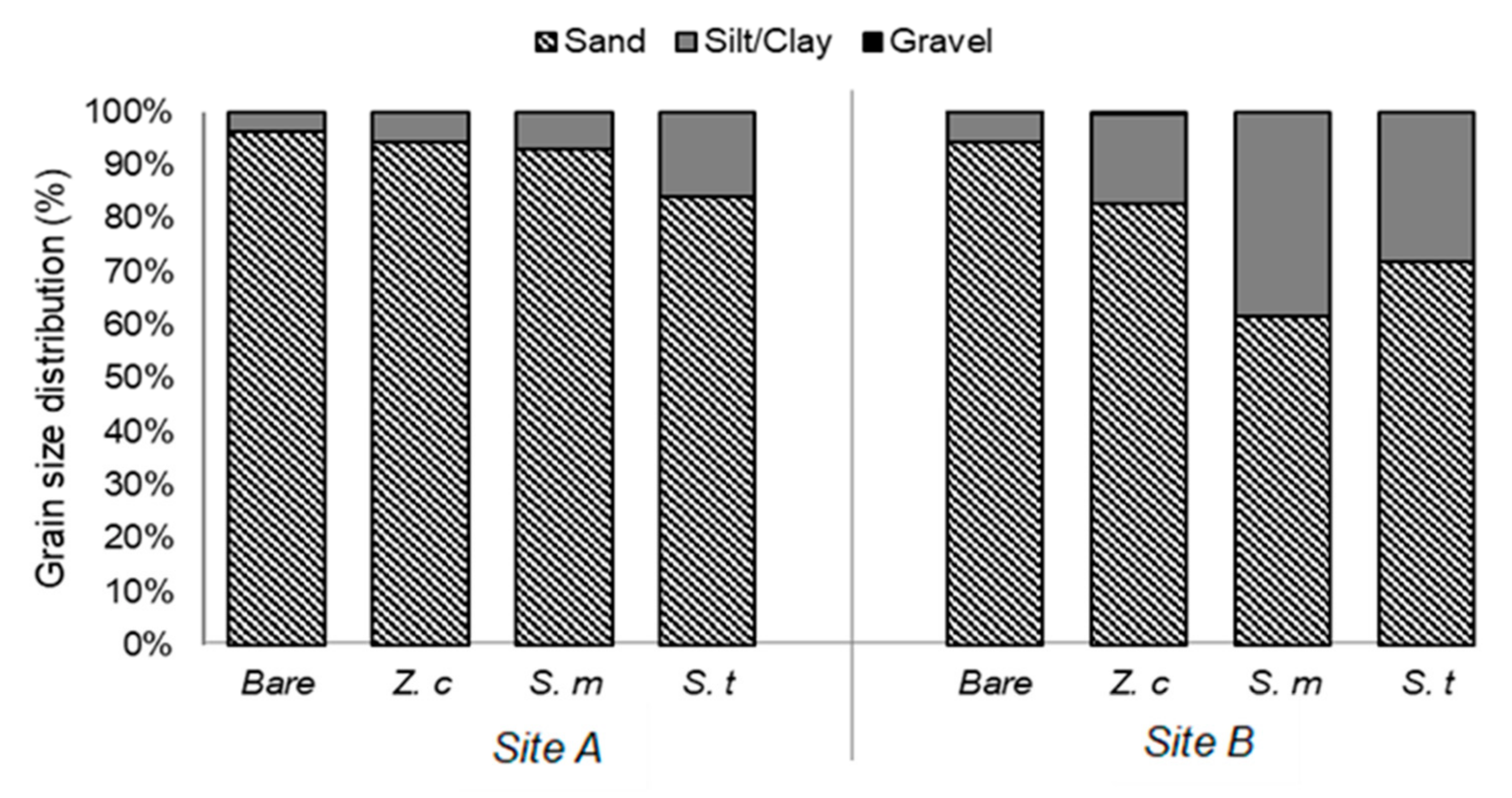
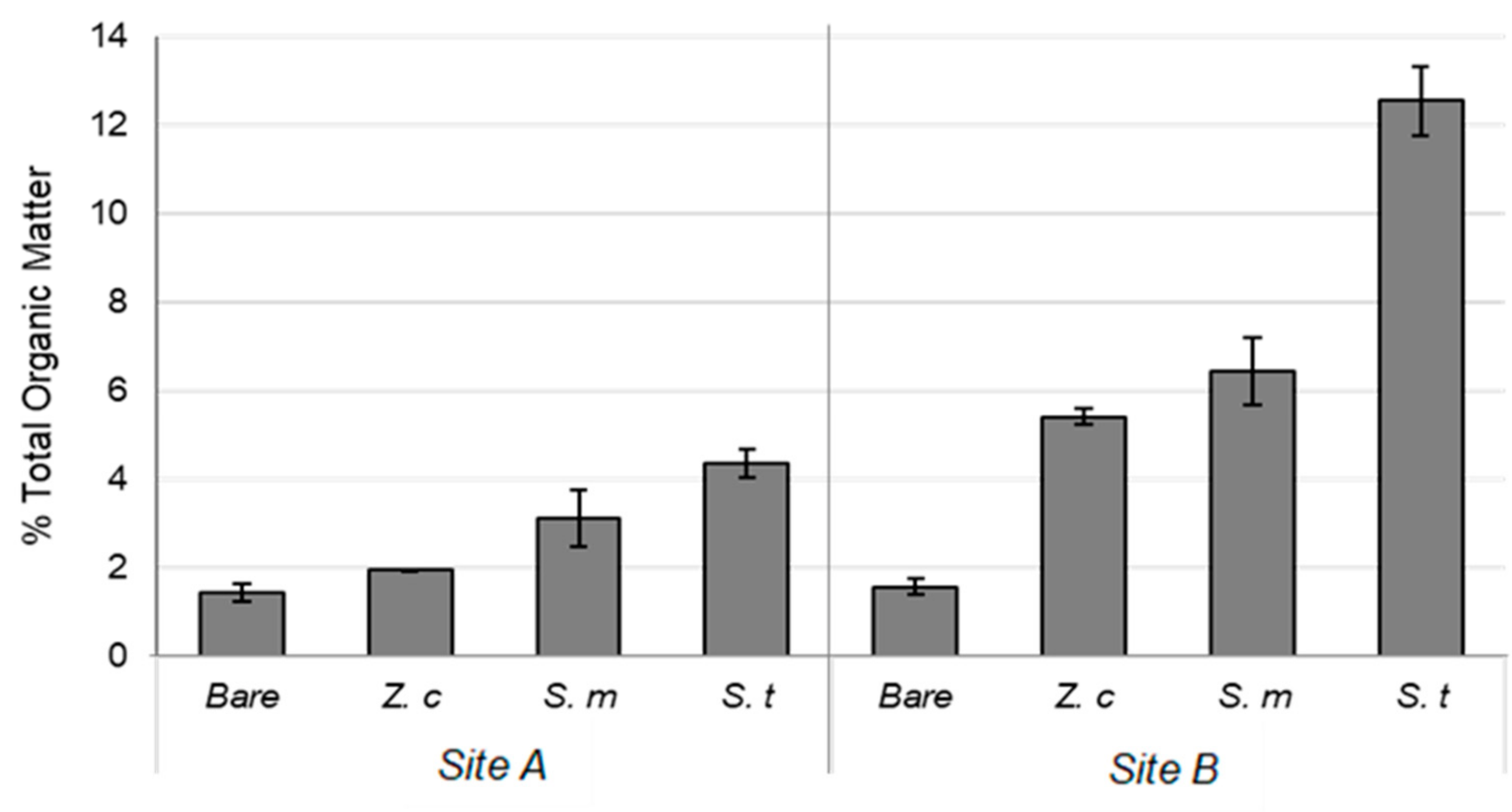
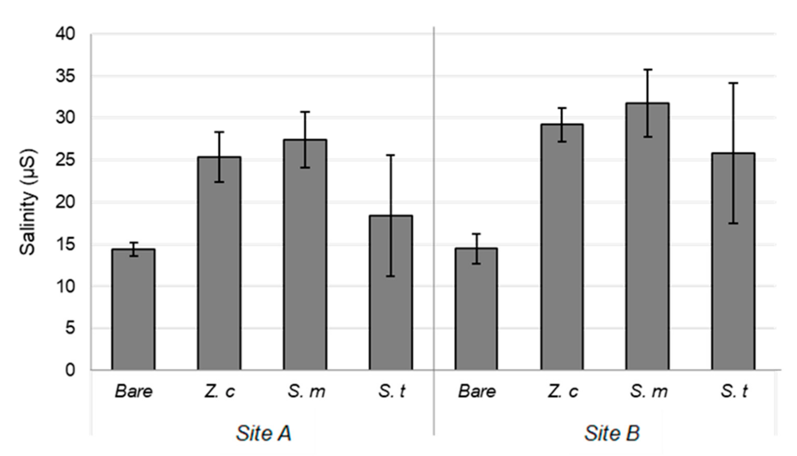
3.1. Sediment Characteristics

The bare sediment had the most sand and least amount of silt/clay, especially in Site B (Figure 2). The grain size and composition of the different rhizosediment for Site A were very similar, only showing a large difference in composition for S. tegetaria, where there was less sand (p = 0.0016) and more silt/clay (p < 0.0001). The differences between the rhizosediment and bare sediment were more noticeable in Site B (bare = 5.57%, Z. capensis = 17.02%, S. maritima = 38.32%, S. tegetaria = 27.99%), the depositional site (silt/clay; p < 0.001, in all cases), than in Site A (bare = 3.80%, Z. capensis = 5.66%, S. maritima = 6.88%, S. tegetaria = 16.02%). Therefore, Site B was generally less sandy than Site A. The bare sediment had similar grain size compositions between the sites (sand; p = 0.9991, silt/clay; p = 0.1449), but rhizosediments had significant differences (silt/clay; p < 0.01, in all cases).
In both sites, TOM increased in the intertidal zone (Z. capensis < S. maritima < S. tegetaria), and bare sediment had the lowest TOM (Figure 3; Site A = 1.46%, Site B = 1.59%). Bare sediment had statistically similar TOM between sites (p = 0.9926). Once again, the differences between the rhizosediment and bare sediment were more noticeable in Site B (Z. capensis = 5.43%, S. maritima = 6.46%, S. tegetaria = 12.56%), the depositional site (p < 0.001, in all cases). At Site A, however, there was no difference in TOM between Z. capensis and the bare sediment in Site A (p < 0.2173).
Salinity did not increase with intertidal range, as would be expected, but the highest salinity is instead found for S. maritima (Figure 4) though not much statistical difference could be shown between the bare sediment and rhizosediment in Site A (p > 0.06, in all cases). Bare sediment, however, showed lower salinity in both sites (Site A = 14.4 µS, Site B = 14.5), even though bare sediment was collected above the S. maritima (highest intertidal) in the case of Site A. At Site B the salinity of the bare sediment was not significantly different to the rhizosediment of S. tegetaria (p = 0.1541). The bare sediment and the rhizosediment all had statistically similar salinity between the sites (bare sediment; p = 1.000 and rhizosediment; p > 0.5, respectively).

3.2. Total Metal Concentrations

Metal concentrations differed between vegetation type, metals, and sites. The different metals had different concentrations (Table 1). Notably, where statistically significant differences occur between concentrations in bare sediment and the other rhizosediment, it was always higher in the rhizosediment than the bare sediment. Differences were more notable in Site B compared to Site A, where only Ni was statistically similar to the bare sediment for Z. capensis. However, the margin is very slight as p = 0.0742. Regarding Site A, Z. capensis rhizosediments was the most similar to the bare sediment, statistically, with the exception of Ni and Cu, which was not the case for Site B (p = 0.0049). The notable differences were between Fe and Mn for S. maritima and S. tegetaria, and Cr for S. maritima. Comparably, the metal concentrations in Site A were less than Site B, for the rhizosediment sites. However, there were a couple of exceptions for Ni. Spartina maritima also showed statistical similarities for Mn and Zn between the sites, even though the means for Site A was lower than Site B—the similarities could be attributed to an overlap in the range resulting in a high standard deviation (p = 0.0756 and p = 0.1794, respectively). Metal concentrations between sites for bare sediment were statistically similar, again, with the only exception being Ni (p = 0.0022).

3.3. nMDS Evaluation of Bare versus Vegetated Rhizosediment

The multivariate analysis showed patterns akin to the sediment characteristics, specifically grain size and salinity for the bare sediment, and rhizosediment of S. maritima and Z. capensis, while TOM was only closely related to S. tegetaria in Site B (Figure 5a,b). In Site A it was more difficult to determine, as the sediment characteristics were not as statistically distinct as in Site B. Larger differences between the communities were shown for Site B (Figure 5b) compared to Site A (Figure 5), but each site had well-defined communities. Overlaps occurred for Z. capensis and S. maritima in Site A and, S. tegetaria and Z. capensis in Site B.

4. Discussion

4.1. Sediment Characteristics

There were distinct differences between the sediment properties of the two sites (Site A and Site B) in the estuary, as well as between the rhizosediment of the vegetation types. Sand was dominant in both sites, but Site A had remarkably more sand than Site B. The finer silt/clay particles were therefore higher in Site B. However, bare sediment showed similar grain size composition between sites. The bare sediment, Z. capensis rhizosediment, and S. maritima rhizosediment in Site A also showed remarkably similar grain size compositions, while Site B’s sediment was more distinct between vegetation types. Nevertheless, bare sediment showed the lowest silt/clay content and the highest sand content in Site B. A large sandbank, most likely succeeding the construction of Wylde Bridge, was largely fluvially driven and deposited by the ebb-directed tidal flow from the sea [38,39]. The natural and man-made geography in this section (around Site B) of the estuary resulted in the slackening of the downstream flow [38], contributing to the build-up of finer-grained sediment in Site B, and a steeper incline between the subtidal and upper intertidal vegetation. The intertidal macrophytes trap more sediment as the flood tide recedes, increasing the presence of fine-grained sediment, particularly for S. maritima and S. tegetaria, higher up the intertidal zone [40]. The silt/clay fraction in this area is comparatively high, even though there is little input of fine-grained sediment into the estuary [41]. Site B is therefore considered a depositional site, which traps fine particles flowing downstream.
Total Organic Matter (TOM) increased with the intertidal zonation, that is, bare sediment had the lowest content and S. tegetaria had the highest content. Similarly to the silt/clay content, TOM was higher in Site B than in Site A, due to the same trapping mechanics of particles at the large sandbank. Site B (Tippers Creek) is a well-known collection site, trapping particles from upstream, and so has been recommended for monitoring [42]. Els reported %TOM for winter, one year prior to this study, and found notably lower TOM for all three of the plant species for the same sites [43]. The exception was S. tegetaria in Site B, which instead increased by a factor of approximately 1.5. Watling and Watling and Nel et al. both concluded that Tippers’ Creek is incompletely flushed by tidal action, resulting in the build-up of contaminants over time [44,45]. Organic particles deposited by the flood tide may become trapped in the higher intertidal zone colonised by S. tegetaria, due to higher surface elevation on the sandbank [46].
Sediment salinity was very similar in the upstream Site A and the downstream Site B. Site B had a larger intertidal range; thus, the vegetation types were further apart. Rhizosediment of S. tegetaria in particular had more variability in salinity measurements, which could indicate some extended evaporation periods in some areas in the upper intertidal zone. Higher salinity in the lower intertidal—subtidal zones will be washed more frequently by saline water from the flood tide at lower elevations, while higher intertidal—supratidal species are inundated less frequently and for shorter periods of time [46]. Bornman et al. did not find that sediment salinity was a key driver in their study on sea-level rise and intertidal salt marshes in the Swartkops Estuary since recorded values were very low [40]. However, they expected water column salinity to be lower compared to the natural state, as increasing freshwater input (i.e., stormwater run-off, treated sewerage water) enters into the catchment. This study’s values correspond to the range of salinity found in Figure 4, which indicates that salinity is unlikely to be a driver of metal accumulation.

4.2. Metal Concentration

In this study, the vegetated rhizosediment contained more metals than the bare sediment. That is, metal concentrations had the following general trend: bare < Z. capensis rhizosediment < S. maritima rhizosediment < S. tegetaria rhizosediment. This trend has been found in other studies around the world (e.g., Pedro et al. [5]). However, this study also includes a comparison between a depositional and non-depositional site. Studies suggest that wetland plants predominantly accumulate metals within their rhizosphere and that they have an influence on the bioavailability of metals in sediment, so information on metal accumulation in sediment is important to consider in monitoring health in estuaries [2,15,21,47,48].
The metal concentrations were higher in Site B compared to Site A, which was located further upstream. Although Site A is located closer to the point sources, the topography of the two areas is very different. The riverbank in Site A is unmodified followed by Wylde Bridge further away—Site B is located after the bridge where the sandbank splits the channel into a large, but comparatively shallower creek. The jetties, modified embankment, and sandbank located at Site B effectively traps the currently transported particles, slowed down by the bridges. The accretion of sediment in Site B elevates S. tegetaria and S. maritima on the sandbank and accumulates enriched particles, and with little flushing in the creek, the metals are held in the marsh. Unsurprisingly, various authors have recommended the site for long-term monitoring of metals and other pollutants [42,49]. The results in Table 1 indeed show that the metal load in Site B is much larger than in Site A, particularly on the sandbank where S. tegetaria and S. maritina was located. The higher metal accumulation in Site B occurred despite the fact that Site A was located close to a point source, and that Site B does not contain a point source.
Our results show significantly fewer metals in bare sediment compared to the rhizosediment. Salicornia tegetaria rhizosediments specifically contain 5.6 times more Fe, and 4.8 times more Mn than the bare sediment in Site B (Table 1). Apart from Pb, which had lower concentrations, and Cu with similar concentrations, the Cr, Mn, and Zn concentrations were significantly higher than the concentrations found by Binning and Baird, for the middle and lower reaches of the estuary [26]. Nickel and Cu were in range to the concentrations found in sediments by Nel et al. four to five years prior to this study, in the Swartkops Estuary [44]. However, Fe, Mn, Zn, Cr, and Pb were much higher. Lastly, Phillips et al. found higher concentrations of Pb and Cu and similar Zn concentrations, in rhizosediments, of the Swartkops Estuary [34]. Although older studies indicated an increase in metal concentrations in the Swartkops Estuary [26,45,50], they were not conducted in rhizosediment, but in surface sediment in the channel. Therefore, if a higher concentration is expected in rhizosediment compared to bare or channel sediment (as seen in Table 1), a conclusion on the extent of metal pollution in the estuary cannot be made when compared to the oldest studies, 40 years ago. An enrichment study on the channel sediment is therefore recommended, but our work and that of Phillips et al. indicate that the wetlands in the Swartkops Estuary have been acting as sinks for metal pollution [34].
Bonanno et al. showed that metal translocation and accumulation is often based on the individual species and not their ecological or morphological similarities [51]. Indicating that each plant species should be carefully studied as a potential phytoremediator, biomonitor or metal sink. It is important to consider the metal concentrations in rhizosediment of S. tegetaria, S. maritima, and Z. capensis, due to their dominance in Southern African estuaries, in order to set a baseline of the levels of metals these plants can tolerate. This information is crucial for laboratory-based bioassays, where macrophytes are exposed to different levels of metal concentrations, to determine their tolerance.
Plants can release substances such as root exudates to change the chemical sediment environment and promote metal bioavailability [13]. The uptake and release of exudates highly depend on root structure surface area to volume ratio [52]. Some wetland plants adapt to low-oxygen, waterlogged environments through Radial Oxygen Loss (ROL), by sending oxygen to their rhizosphere [15]. The change from a less reduced environment allows the precipitation of ferric- and Mn-oxide/hydroxides called iron plaque, which often forms a protective layer around the rhizosphere. The oxygenation only extends 0.4–2.5 mm from the rhizosphere and does not affect bulk sediment [53,54]. Iron plaque has been recorded for S. tegetaria, Z. capensis, and S. maritima [15,47,53,55,56], and may contribute to the higher recorded Mn and Fe in the rhizosediments compared to the bare sediment. The precipitation of iron plaque is followed by the co-precipitation of other metals including Zn, Pb, Cu, and Al. This may result in correlations between different metals’ concentrations in the sediment. This would account for the considerably higher concentrations of these metals in the rhizosediment compared to the bare sediment. Martins et al. found that the amount of oxygen pumped to the depths can exceed the consumption, and oxygen can spread into the surrounding bulk sediment [56]. The subsequent immobilisation of metals can increase the capacity of the marsh sediment to accumulate more metals, by providing surface area for adsorption [56]. Radical oxygen loss increases the capacity of salt marsh plants as phytostabilisers, the lack of the process in bare sediment (especially in waterlogged areas) will decrease metal content and increase their leaching (and their toxicity). The highly dense root system of S. maritima may promote more changes to the metal accumulation capacity of the rhizosediment via root exudates compared to the seagrass, Z. capensis and S. tegetaria, which has a much less pronounced root system [52].
Another factor contributing to higher metal accumulation in rhizosediment is the total organic matter (TOM). The higher TOM was comparable with higher metal concentration, and lower TOM with the lower metal concentrations (Table 1 and Figure 3). Organic matter can either act as a source or a sink of metals depending on its solubility and the particular metals [57,58]. Williams et al. indicated that high organic matter presents higher metal accumulation in wetlands [8]. In general, the cationic metals in this study should form insoluble complexes with organic matter. Copper and Pb prefer to form bonds with organic matter [11,59,60], and dissolved Fe3+ and Cr3+ associate well with humic substances. Other metals also adsorb it due to its high specific surface area [61]. High decomposition rates of organic matter can cause the dissolution of Mn and Fe oxides/hydroxides (i.e., dissolve iron plaque), causing rapid anaerobic conditions and higher rates of leaching. Longer inundation times make leaching more prevalent in Z. capensis and S. maritima habitats in the lower marsh. However, simpler aerenchyma tissue in Z. capensis in comparison to more developed aerenchyma tissue in S. maritima greatly decreases metal accumulation in Z. capensis rhizosediment [19]. Nonetheless, all rhizosediment stored significantly more metals than the bare sediment.
Vegetation greatly reduces the energy of shallow wave-currents, trapping suspended particles in the habitat [14,60]. Suspended particles can contain organic matter and fine-grained sediment. Higher percentages of silt and clays in the sediment increase the metal binding capacity of cationic metals onto the negatively charged surfaces [62]. These bonding sites in clays are created by Al oxides, Mn oxides, and Fe oxides [63,64]. Although higher concentrations of these elements were found in sediments containing high metal concentrations, the results were not as well correlated as the TOM. However, sand being more prevalent in Site A is probably the reason why metal concentrations are comparatively lower, and why the different rhizosediment had little difference (Figure 5). Bare sediment, Z. capensis rhizosediment, and S. maritima rhizosediment have similar grain size compositions with >90% sand. However, S. maritima has significantly higher Fe and Mn, indicating the possible formation of root plaque. Spartina spp. have highly developed aerenchyma tissue, maintaining more effective oxygen demands under waterlogged conditions [15]. While S. tegetaria in Site A, the higher clay/silt content played a significant role to sequester higher metal concentrations, in the higher intertidal zone with less frequent anaerobic conditions. The upper intertidal zones (e.g., S. tegetaria habitat) are also less frequently inundated and therefore is less flushed compared to the lower intertidal zones (S. maritima and Z. capensis habitats).
Lastly, sediment salinity did not differ considerably between sites (Figure 4) and vegetation type and was not a driver of metal accumulation, indicated by the direction of the environmental vectors for Site A in Figure 5a. However, higher sediment salinity was associated with S. tegetaria rhizosediment in Site B (Figure 5b). Fritioff et al. found that metals become more bioavailable for submersed plants with decreasing salinity and increasing temperature [65]. A decrease in the salinity in the estuary due to increased effluent input may enhance metal toxicity in the future.

5. Conclusions

This study investigated the metal concentrations in the intertidal sediment of the Swartkops Estuary, South Africa. The metal concentrations show a clear pattern of accumulation favouring the rhizosediment over the bare sediment. Metal concentrations were also higher higher up the intertidal range (i.e., in S. tegetaria) compared to lower down the intertidal rage (i.e., Z. capensis). Depositional sites accumulated higher silt/clay content and organic content, but only for the rhizosediment, while bare sediment was similar between depositional and non-depositional sites. Therefore, it can be concluded that the rhizosediment acts as a sink of metals and that the depositional site without point sources captures the metals more efficiently than the upstream non-depositional site, with closer point sources. Our results indicate that it should be a priority to conserve wetland plants that act as metal sinks, considering the high rate of salt marsh loss locally and globally, and their ability to reduce/prevent metal toxicity.

Author Contributions

Conceptualization, M.A.N. and L.R.D.H.; methodology, M.A.N., L.R.D.H., and G.R.; software, M.A.N.; validation, L.R.D.H. and J.B.A.; formal analysis, M.A.N.; investigation, M.A.N.; resources, L.R.D.H., J.B.A. and G.R.; data curation, M.A.N.; writing—original draft preparation, M.A.N.; writing—review and editing, M.A.N., J.B.A., L.R.D.H., and G.R.; visualization, M.A.N.; supervision, L.R.D.H., J.B.A., and G.R.; project administration, M.A.N.; funding acquisition, J.B.A. and L.R.D.H. All authors have read and agreed to the published version of the manuscript.

Funding

The research was funded by the National Research Foundation (Grant Number: 120406). The first author was supported by a scholarship from the National Research Foundation of South Africa (Grant Number: 116920).

Institutional Review Board Statement

Ethical review and approval were not applicable for this study due to no involvement of human or animal subjects.

Informed Consent Statement

Patient consent was not applicable due to no involvement of human subjects.

Data Availability Statement

The raw data supporting the conclusions of this article will be made available by the authors, without undue reservation.

Acknowledgments

This work was supported by the Shallow Marine and Coastal Research Infrastructure (SMCRI) platform hosted by the South African Environmental Observation Network Elwandle Node (SAEON). The authors also wish to thank the Shallow Water Ecosystem research group (funded by UID 84375DSI/NRF Research Chair) for assistance in the laboratory and field.

Conflicts of Interest

The authors declare no conflict of interest. The funders had no role in the design of the study; in the collection, analyses, or interpretation of data; in the writing of the manuscript, or in the decision to publish the results.

References

  1. Van Niekerk, L.; Adams, J.B.; Bate, G.C.; Forbes, A.T.; Forbes, N.T.; Huizinga, P.; Lamberth, S.J.; MacKay, C.F.; Petersen, C.; Taljaard, S.; et al. Country-Wide Assessment of Estuary Health: An Approach for Integrating Pressures and Ecosystem Response in a Data Limited Environment. Estuar. Coast. Shelf Sci. 2013, 130, 239–251. [Google Scholar] [CrossRef]
  2. Doyle, M.; Otte, M. Organism-Induced Accumulation of Iron, Zinc and Arsenic in Wetland Soils. Environ. Pollut. 1997, 96, 1–11. [Google Scholar] [CrossRef]
  3. Reboreda, R.; Caçador, I. Halophyte Vegetation Influences in Salt Marsh Retention Capacity for Heavy Metals. Environ. Pollut. 2007, 146, 147–154. [Google Scholar] [CrossRef] [PubMed]
  4. Anjum, N.A.; Duarte, B.; Caçador, I.; Sleimi, N.; Duarte, A.C.; Pereira, E. Biophysical and Biochemical Markers of Metal/Metalloid-Impacts in Salt Marsh Halophytes and Their Implications. Front. Environ. Sci. 2016, 4, 24. [Google Scholar] [CrossRef] [Green Version]
  5. Pedro, S.; Duarte, B.; Raposo, P.; Almeida, D.; Caçador, I. Metal Speciation in Salt Marsh Sediments: Influence of Halophyte Vegetation in Salt Marshes with Different Morphology. Estuar. Coast. Shelf Sci. 2015, 167, 248–255. [Google Scholar] [CrossRef]
  6. Bonanno, G.; Vymazal, J.; Cirelli, G.L. Translocation, Accumulation and Bioindication of Trace Elements in Wetland Plants. Sci. Total Environ. 2018, 631–632, 252–261. [Google Scholar] [CrossRef]
  7. de Souza Machado, A.A.; Spencer, K.; Kloas, W.; Toffolon, M.; Zarfl, C. Metal Fate and Effects in Estuaries: A Review and Conceptual Model for Better Understanding of Toxicity. Sci. Total Environ. 2016, 541, 268–281. [Google Scholar] [CrossRef]
  8. Williams, T.P.; Bubb, J.M.; Lester, J.N. Metal Accumulation within Salt Marsh Environments: A Review. Mar. Pollut. Bull. 1994, 28, 277–290. [Google Scholar] [CrossRef]
  9. Caçador, I.; Vale, C.; Catarino, F. Seasonal Variation of Zn, Pb, Cu and Cd Concentrations in the Root- Sediment System of Spartina Maritima and Halimione Portulacoides from Tagus Estuary Salt Marshes. Mar. Environ. Res. 2000, 49, 279–290. [Google Scholar] [CrossRef]
  10. Bonanno, G.; Raccuia, S.A. Comparative Assessment of Trace Element Accumulation and Bioindication in Seagrasses Posidonia Oceanica, Cymodocea Nodosa and Halophila Stipulacea. Mar. Pollut. Bull. 2018, 131, 260–266. [Google Scholar] [CrossRef]
  11. Duarte, B.; Caetano, M.; Almeida, P.R.; Vale, C.; Caçador, I. Accumulation and Biological Cycling of Heavy Metal in Four Salt Marsh Species, from Tagus Estuary (Portugal). Environ. Pollut. 2010, 158, 1661–1668. [Google Scholar] [CrossRef] [PubMed]
  12. Bonanno, G.; Vymazal, J. Compartmentalization of Potentially Hazardous Elements in Macrophytes: Insights into Capacity and Efficiency of Accumulation. J. Geochem. Explor. 2017, 181, 22–30. [Google Scholar] [CrossRef]
  13. du Laing, G.; Rinklebe, J.; Vandecasteele, B.; Meers, E.; Tack, F.M.G. Trace Metal Behaviour in Estuarine and Riverine Floodplain Soils and Sediments: A Review. Sci. Total Environ. 2009, 407, 3972–3985. [Google Scholar] [CrossRef] [PubMed]
  14. Ward, L.G.; Kemp, M.W.; Boynton, W.R. The Influence of Waves and Seagrass Communities on Suspended Particulates in an Estuarine Embayment. Mar. Geol. 1984, 59, 85–103. [Google Scholar] [CrossRef]
  15. Maricle, B.R.; Lee, R.W. Aerenchyma Development and Oxygen Transport in the Estuarine Cordgrasses Spartina Alterniflora and S. Anglica. Aquat. Bot. 2002, 74, 109–120. [Google Scholar] [CrossRef]
  16. Yang, J.; Ye, Z. Metal Accumulation and Tolerance in Wetland Plants. Front. Biol. China 2009, 4, 282–288. [Google Scholar] [CrossRef]
  17. Pezeshki, S.R.; DeLaune, R.D. Soil Oxidation-Reduction in Wetlands and Its Impact on Plant Functioning. Biology 2012, 1, 196–221. [Google Scholar] [CrossRef] [Green Version]
  18. Fakoya, O.T.; Oluyemi, E.A.; Olabanji, I.O.; Eludoyin, A.O.; Makinde, O.W.; Oyinloye, J.A. Seasonal Variation of Heavy Metal Speciation in Soil and Stream Sediments from Hospital Waste Dumpsite in Ilesa, Southwestern Nigeria. Afr. J. Environ. Sci. Technol. 2018, 12, 312–322. [Google Scholar] [CrossRef]
  19. Reboreda, R.; Caçador, I. Copper, Zinc and Lead Speciation in Salt Marsh Sediments Colonised by Halimione Portulacoides and Spartina Maritima. Chemosphere 2007, 69, 1655–1661. [Google Scholar] [CrossRef]
  20. Peppicelli, C.; Cleall, P.; Sapsford, D.; Harbottle, M. Changes in Metal Speciation and Mobility during Electrokinetic Treatment of Industrial Wastes: Implications for Remediation and Resource Recovery. Sci. Total Environ. 2018, 624, 1488–1503. [Google Scholar] [CrossRef]
  21. Kabata-Pendias, A. Trace Elements in Soils and Plants, 4th ed.; CRC Press: Boca Raton, FL, USA, 2011; ISBN 9781420093681. [Google Scholar]
  22. Colloty, B.M.; Adams, J.B.; Bate, G.C. The Use of a Botanical Importance Rating to Assess Changes in the Flora of the Swartkops Estuary over Time. Water SA 2000, 26, 171–180. [Google Scholar]
  23. van Niekerk, L.; Adams, J.B.; Lamberth, S.J.; MacKay, C.F.; Taljaard, S.; Turpie, J.K.; Raimondo, D.C. South African National Biodiversity Assessment 2018: Technical Report. Volume 3: Estuarine Realm; CSIR: Stellenbosch, South Africa, 2019; Volume 3. [Google Scholar]
  24. Enviro-Fish Africa. Swartkops Integrated Environmental Management Plan; CAPE: Port Elizabeth, South Africa, 2009. [Google Scholar]
  25. Enviro-Fish Africa. Integrated Management Plan: Swartkops Estuary and the Swartkops River Valley and Aloes Nature Reserves; CAPE: Grahamstown, South Africa, 2011. [Google Scholar]
  26. Binning, K.; Baird, D. Survey of Heavy Metals in the Sediments of the Swartkops River Estuary, Port Elizabeth South Africa. Water SA 2001, 27, 461–466. [Google Scholar] [CrossRef] [Green Version]
  27. Fourqurean, J.W.; Johnson, B.; Kauffman, J.B.; Kennedy, H.; Lovelock, C.E.; Megonigal, J.P.; Rahman, A.; Saintilan, N.; Simard, M. Coastal Blue Carbon; Howard, J., Hoyt, S., Isensee, K., Emily, P., Telszewski, M., Eds.; International Union for Conservation of Nature: Arlington, VA, USA, 2017; ISBN 9782831717623. [Google Scholar]
  28. Wentworth, C.K. A Scale of Grade and Class Terms for Clastic Sediments. J. Geol. 1922, 30, 377–392. [Google Scholar] [CrossRef]
  29. Buchanan, J.B. Sediment Analysis. In Methods for the Study of Marine Benthos; Holme, N.A., McIntyre, A.D., Eds.; Blackwell: Oxford, UK, 1984; pp. 41–65. [Google Scholar]
  30. Briggs, D. Soils: Sources and Methods in Geography; Butterworths: London, UK, 1977; ISBN 0408709111. [Google Scholar]
  31. Veres, D.S. A Comparitive Study between Loss on Ignition and Total Carbon Analysis on Minerogenic Sediments. Studia Univ. Babes-Bolyai 2002, 67, 171–182. [Google Scholar] [CrossRef]
  32. Bernard, R.O. Handbook of Standard Soil Testing Methods for Advisory Purposes; Sediment Science Society of South Africa: Pretoria, South Africa, 1990; ISBN 0620148004. [Google Scholar]
  33. du Laing, G.; Tack, F.M.G.; Verloo, M.G. Performance of Selected Destruction Methods for the Determination of Heavy Metals in Reed Plants (Phragmites australis). Anal. Chim. Acta 2003, 497, 191–198. [Google Scholar] [CrossRef]
  34. Phillips, D.P.; Human, L.R.D.; Adams, J.B. Wetland Plants as Indicators of Heavy Metal Contamination. Mar. Pollut. Bull. 2015, 92, 227–232. [Google Scholar] [CrossRef]
  35. Vilhena, J.C.E.; Amorim, A.; Ribeiro, L.; Duarte, B.; Pombo, M. Baseline Study of Trace Element Concentrations in Sediments of the Intertidal Zone of Amazonian Oceanic Beaches. Front. Mar. Sci. 2021, 8, 570. [Google Scholar] [CrossRef]
  36. Montero Alvarez, A.; Estévez Alvarez, J.R.; Padilla Alvarez, R. Heavy Metal Analysis of Rainwaters: A Comparison of TXRF and ASV Analytical Capabilities. J. Radioanal. Nucl. Chem. 2007, 273, 427–433. [Google Scholar] [CrossRef]
  37. Matusiak, K.; Skoczen, A.; Setkowicz, Z.; Kubala-Kukus, A.; Stabrawa, I.; Ciarach, M.; Janeczko, K.; Jung, A.; Chwiej, J. The Elemental Changes Occurring in the Rat Liver after Exposure to PEG-Coated Iron Oxide Nanoparticles: Total Reflection x-Ray Fluorescence (TXRF) Spectroscopy Study. Nanotoxicology 2017, 11, 1225–1236. [Google Scholar] [CrossRef]
  38. Esterhuysen, K.; Rust, I.C. Channel Migration in the Lower Swartkops Estuary. S. Afr. J. Sci. 1987, 83, 521–525. [Google Scholar]
  39. Reddering, J.S.V.; Esterhuysen, K.; Rust, I.C. The Sedimentary Ecology of the Swartkops Estuary; University of Port Elizabeth: Gqeberha, South Africa, 1981; ISBN 0869882589. [Google Scholar]
  40. Bornman, T.G.; Schmidt, J.; Adams, J.B.; Mfikili, A.N.; Farre, R.E.; Smit, A.J. Relative Sea-Level Rise and the Potential for Subsidence of the Swartkops Estuary Intertidal Salt Marshes, South Africa. South Afr. J. Bot. 2016, 107, 91–100. [Google Scholar] [CrossRef]
  41. Reddering, J.S.; Esterhuysen, K. The Swartkops Estuary: Physical Description and History. Swart. Estuary 1988, 7–15. [Google Scholar]
  42. Adams, J.B.; Pretorius, L.; Snow, G.C. Deterioration in the Water Quality of an Urbanised Estuary with Recommendations for Improvement. Water SA 2019, 45, 86–96. [Google Scholar] [CrossRef] [Green Version]
  43. Els, J. Carbon and Nutrient Storage of the Swartkops Estuary Salt Marsh and Seagrass Habitats; Nelson Mandela University: Port Elizabeth, South Africa, 2020. [Google Scholar]
  44. Nel, L.; Strydom, N.A.; Bouwman, H. Preliminary Assessment of Contaminants in the Sediment and Organisms of the Swartkops Estuary, South Africa. Mar. Pollut. Bull. 2015, 101, 878–885. [Google Scholar] [CrossRef]
  45. Watling, R.J.; Watling, H.R. Metal Surveys in South African Estuaries. I. Swartkops River. Water SA 1982, 8, 26. [Google Scholar]
  46. Veldkornet, D.A.; Potts, A.J.; Adams, J.B. The Distribution of Salt Marsh Macrophyte Species in Relation to Physicochemical Variables. S. Afr. J. Bot. 2016, 107, 84–90. [Google Scholar] [CrossRef]
  47. Smillie, C. Salicornia Spp. as a Biomonitor of Cu and Zn in Salt Marsh Sediments. Ecol. Indic. 2015, 56, 70–78. [Google Scholar] [CrossRef]
  48. Furtado, B.U.; Golebiewski, M.; Skorupa, M.; Hulisz, P.; Hrynkiewicz, K. Bacterial and Fungal Endophytic Microbiomes of Salicornia Europaea. Appl. Environ. Microbiol. 2019, 85, 1–18. [Google Scholar] [CrossRef] [Green Version]
  49. Nel, M.A.; Rubidge, G.; Adams, J.B.; Human, L.R.D. Rhizosediments of Salicornia Tegetaria Indicate Metal Contamination in the Intertidal Estuary Zone. Front. Environ. Sci. 2020, 8, 175. [Google Scholar] [CrossRef]
  50. Watling, R.J.; Watling, H.R. Metal Surveys in Southern African Estuaries: 1. Swartkops Estuary. CSIR Spec. Rep. FIS 1979, 183. [Google Scholar]
  51. Bonanno, G.; Borg, J.A.; di Martino, V. Levels of Heavy Metals in Wetland and Marine Vascular Plants and Their Biomonitoring Potential: A Comparative Assessment. Sci. Total Environ. 2017, 576, 796–806. [Google Scholar] [CrossRef] [PubMed]
  52. Wang, H.; Inukai, Y.; Yamauchi, A. Root Development and Nutrient Uptake. Crit. Rev. Plant Sci. 2006, 25, 279–301. [Google Scholar] [CrossRef]
  53. Koop-Jakobsen, K.; Fischer, J.; Wenzhöfer, F. Survey of Sediment Oxygenation in Rhizospheres of the Saltmarsh Grass - Spartina Anglica. Sci. Total Environ. 2017, 589, 191–199. [Google Scholar] [CrossRef] [PubMed]
  54. Holmer, M.; Gribsholt, B.; Kristensen, E. Effects of Sea Level Rise on Growth of Spartina Anglica and Oxygen Dynamics in Rhizosphere and Salt Marsh Sediments. Mar. Ecol. Prog. Ser. 2002, 225, 197–204. [Google Scholar] [CrossRef]
  55. Frederiksen, M.S.; Glud, R.N. Oxygen Dynamics in the Rhizosphere of Zostera Marina: A Two-Dimensional Planar Optode Study. Limnol. Oceanogr. 2006, 51, 1072–1083. [Google Scholar] [CrossRef] [Green Version]
  56. Martins, M.; Ferreira, A.M.; Vale, C. The Influence of Sarcocornia Fruticosa on Retention of PAHs in Salt Marsh Sediments (Sado Estuary, Portugal). Chemosphere 2008, 71, 1599–1606. [Google Scholar] [CrossRef]
  57. Tranvik, L.J. Dystrophy in Freshwater Systems; Elsevier Inc.: Amsterdam, The Netherlands, 2014; ISBN 9780124095489. [Google Scholar]
  58. Violante, A.; Cozzolino, V.; Perelomov, L.; Caporale, A.G.; Pigna, M. Mobility and Bioavailability of Heavy Metals and Metalloids in Soil Environments. J. Soil Sci. Plant Nutr. 2010, 10, 268–292. [Google Scholar] [CrossRef] [Green Version]
  59. Wyatt, K.H.; Stevenson, R.J. Effects of Acidification and Alkalinization on a Periphytic Algal Community in an Alaskan Wetland. Wetlands 2010, 30, 1193–1202. [Google Scholar] [CrossRef]
  60. Human, L.; Feijão, E.; de Carvalho, R.C.; Caçador, I.; Reis-Santos, P.; Fonseca, V.; Duarte, B. Mediterranean Salt Marsh Sediment Metal Speciation and Bioavailability Changes Induced by the Spreading of Non-Indigenous Spartina Patens. Estuar. Coast. Shelf Sci. 2020, 243, 1–9. [Google Scholar] [CrossRef]
  61. Lin, J.G.; Chen, S.Y.; Su, C.R. Assessment of Sediment Toxicity by Metal Speciation in Different Particle-Size Fractions of River Sediment. Water Sci. Technol. 2003, 47, 233–241. [Google Scholar] [CrossRef]
  62. Ujević, I.; Odžak, N.; Barić, A. Trace Metal Accumulation in Different Grain Size Fractions of the Sediments from a Semi-Enclosed Bay Heavily Contaminated by Urban and Industrial Wastewaters. Water Res. 2000, 34, 3055–3061. [Google Scholar] [CrossRef]
  63. Elderfield, H.; Hepworth, A.; Edwards, P.N.; Holliday, L.M. Zinc in the Conwy River and Estuary. Estuar. Coast. Mar. Sci. 1979, 9, 403–422. [Google Scholar] [CrossRef]
  64. Talbot, M.M.J.F. Trace Metals in the Marine Environment and Their Effect on Nitrogen Cycling; Nelson Mandela University: Port Elizabeth, South Africa, 1988. [Google Scholar]
  65. Fritioff, Å.; Kautsky, L.; Greger, M. Influence of Temperature and Salinity on Heavy Metal Uptake by Submersed Plants. Environ. Pollut. 2005, 133, 265–274. [Google Scholar] [CrossRef] [PubMed]
Figure 1. Locations of the sampling sites: (Site A) Markman Canal and (Site B) Tipper’s Creek.
Sustainability 14 03679 g001
Figure 2. Grain size distribution in rhizosediment (vegetated) and bare sediment (unvegetated) of Site A and Site B; where Z.c = Z. capensis, S.m = S. maritima, and S.t = S. tegetaria.
Sustainability 14 03679 g002
Figure 3. Total Organic Matter (TOM) (%) in the rhizosediment and bare mudflats of Site A and Site B; where Z.c = Z. capensis, S.m = S. maritima, and S.t = S. tegetaria (mean ± SD, N = 3).
Sustainability 14 03679 g003
Figure 4. Salinity (µS) in the rhizosediment and bare mudflats of Site A and Site B; where Z.c = Z. capensis, S.m = S. maritima, and S.t = S. tegetaria (mean ± SD, N = 3).
Sustainability 14 03679 g004
Figure 5. Non-metric multidimensional scaling (nMDS) ordination plots based on Euclidean distances of the vegetation types for bare (), Z. capensis (), S. maritima (), and S. tegetaria (), at (a) Site A and (b) Site B.
Sustainability 14 03679 g005
Table 1. Average metal concentrations (µg.g−1 dry weight ± SD) in the surface of vegetated (rhizosediment) and unvegetated (bare) sediment. An asterisk (*) indicates significant differences between the bare mudflat with the different rhizosediments, of the same site and metal (p < 0.05; N = 3). An arrow indicates if the values are significantly higher (↑) or lower (↓).
SitesMetals
(µg.g−1)
UnvegetatedRhizosediment
Bare MudflatZ. capensisS. maritimaS. tegetaria
Site AFe3468 ± 3853152 ± 171↑5407 ± 985 *↑6923 ± 1222 *
Mn31.5 ± 4.130.4 ± 2.5↑63.7 ± 14.2 *↑112.9 ± 28.6 *
Zn48.8 ± 12.738.1 ± 0.857.4 ± 3.853.7 ± 1.8
Cr8.5 ± 1.110.6 ± 0.5↑19.0 ± 4.0 *11.6 ± 1.7
Pb3.9 ± 0.62.8 ± 1.05.2 ± 1.37.1 ± 1.9
Ni0.9 ± 0.5↑4.1 ± 1.7 *1.2 ± 0.41.2 ± 0.3
Cu2.9 ± 0.7↑1.4 ± 0.2 *2.9 ± 0.73.0 ± 0.4
Site BFe5120± 223↑14073 ± 341 *↑19445 ± 2 850 *↑28947 ± 858 *
Mn29.3 ± 1.8↑76.8 ± 10.4 *↑108.6 ± 21.2 *↑367.2 ± 34.4 *
Zn51.2 ± 2.6↑96.7 ± 16.0 *↑81.0 ± 10.3 *↑128.2 ± 9.0 *
Cr10.3 ± 0.7↑36.8 ± 2.3 *↑37.5 ± 4.1 *↑72.1 ± 1.5 *
Pb7.1 ± 0.9↑29.8 ± 5.5 *↑30.3 ± 5.0 *↑59.0 ± 1.5 *
Ni3.5 ± 0.19.6 ± 0.7↑11.2 ± 1.8 *↑21.2 ± 0.7 *
Cu3.5 ± 0.1↑11.6 ± 0.6 *↑8.7 ± 1.2 *↑13.9 ± 0.8 *
Publisher’s Note: MDPI stays neutral with regard to jurisdictional claims in published maps and institutional affiliations.

