Soil Erosion and Deposition in a Taiwanese Watershed Using USPED

Abstract

Soil erosion is a global problem that has been exacerbated in recent decades by global warming and the increased frequency of extreme weather events. It is also a global issue addressed by the United Nations’ Sustainable Development Goal #15 that seeks to recover degraded land and create a world free of land degradation by 2030. In this study, we used the Unit Stream Power-based Erosion Deposition (USPED) model to investigate the distribution of soil erosion and deposition in an important reservoir watershed in Taiwan, which is known to have a high risk of sediment hazard. We found the average soil erosion rate to be 136.4 Mg/ha/year using the model’s recommended m = 1.3 and n = 1.2 empirical coefficients for a combined occurrence of sheet and rill erosion. Additionally, we selected the Sule sub-watershed and the Kala area as examples to illustrate the pattern of soil erosion and deposition and their relationship to rivers, roadways, and anthropogenic activity, and 3D terrain was employed to further enhance visualization of the model output. It was estimated that 12.6% of eroded soil was deposited with a 200 m buffer of the rivers in the watershed and might be swept into the river system by the next typhoon, torrential rain, landslide, or earthquake. In comparison to previous USLE- and RUSLE-based soil erosion modeling in the same research area, our USPED modeling is unique in that it included the amount and distribution of soil deposition. This successful implementation of USPED in Taiwan establishes a new modeling alternative in addition to the widely used USLE and RUSLE models. The findings can be used to direct future erosion pin placement in the research area, allowing for improved monitoring of sediment movement and avoiding sediment hazards.

1. Introduction

Soil erosion is a global problem that has been aggravated by global warming and the increased occurrence of extreme weather events in the last several decades. In accordance with the United Nations’ Sustainable Development Goal (SDG) #15 (life on land), soil is essential to all forms of life on land. One of the SDG’s objectives is to combat desertification by 2030 and restore degraded land and soil, particularly in areas affected by desertification, drought, and flooding, and work toward achieving a world devoid of land degradation. In addition, the loss of valuable soil is associated with a reduction in the functioning of the ecosystem as well as an increase in CO₂ levels in the atmosphere.

When analyzing soil erosion in a watershed, the universal soil loss equation (USLE) and the revised universal soil loss equation (RUSLE) are the most common models used by researchers around the world, accounting for 13.9% and 17.1% of the literature published between 1994 and 2017 in the Scopus database, respectively [1]. The predominant use of USLE and RUSLE is also true in Taiwan for soil erosion analysis [2,3,4,5,6,7,8,9,10,11]. However, USLE or RUSLE can only model the amount of soil erosion in watersheds; they cannot simulate the movement of sediments and where the soil is deposited in the watersheds.

On the other hand, Mitasova et al. [12,13] developed the Unit Stream Power-based Erosion Deposition (USPED) model that was able to model both erosion and deposition as divergence of sediment flow, effectively compensating for the shortcomings of the USLE and RUSLE models. Although USPED accounts for less than 0.7% of all soil erosion modeling studies in the Global Applications of Soil Erosion Modelling Tracker (GASEMT) database [1], many researchers have noted good results in their findings. For example, Borrelli et al. [14] used USPED (m = 1.3 and n = 1.2) to forecast the effect of tree removal on soil erosion in a central Italian intermountain watershed. They discovered that the net soil erosion rate for the undisturbed forest area was 0.34 Mg/ha/year while disturbed forest land had a rate of 5.34 Mg/ha/year. To validate their findings, they planted metallic stakes in a 1.97 hectare experimental watershed. Gross erosion was measured at 3.8 mm/year with a predicted rate of 2.1 mm/year. More recently, Gioia et al. [15] utilized USPED to forecast the location of linear erosion in a 7 km² watershed in southern Italy’s Apennines and discovered that the USPED model predicted the location of linear erosion quite reliably. Similarly, Domingues et al. [16] used USPED and genetic algorithm to optimize the placement and size of forest restoration zones. Also, USPED was used by Leh et al. [17] to examine the effect of land use change on soil erosion risk, and by Liu et al. [18] to model the effect of land cover change on carbon dynamics. Additionally, Skagen et al. [19] used USPED to predict sediment accretion in wetlands in North America’s interior regions and assessed the relative contributions of precipitation and land use. Young et al. [20] investigated the effect of soil organic carbon (SOC) redistribution on soil productivity and crop yield in agricultural fields in the Midwest of the US. Additionally, Honek et al. [21] used USPED to simulate siltation and predicted the lifespan of a small reservoir.

Despite the fact that all these studies gave examples of USPED model applications, the geographic scope of the applications is still quite limited. The limited geographic scope of the model impacts its usefulness. A full assessment of the USPED model as an effective soil erosion modeling tool is hampered by the model’s lower number of reported studies compared to other soil erosion models. Several other issues such as empirical coefficient selection across watersheds and climate zones also need to be addressed.

Taiwan, for example, has never employed USPED-based modeling to model watersheds in the past. As such, the purpose of this work was to apply USPED to the Shihmen Reservoir watershed in Taiwan and to compare the results with those from prior USLE-based assessments and erosion pin measurements. The USPED results included not only soil erosion, as reported by USLE and RUSLE models, but also the amount and distribution of soil deposition. Additionally, the Sule sub-watershed and the Kala area were also used as illustrations of the pattern of soil erosion and deposition and their relationship to rivers, roadways, and anthropogenic activity. To improve the visualization of the model output, three-dimensional landscape was used. The goal is to create a new modeling option in Taiwan, in addition to the widely used USLE and RUSLE models.

2. Material and Methods

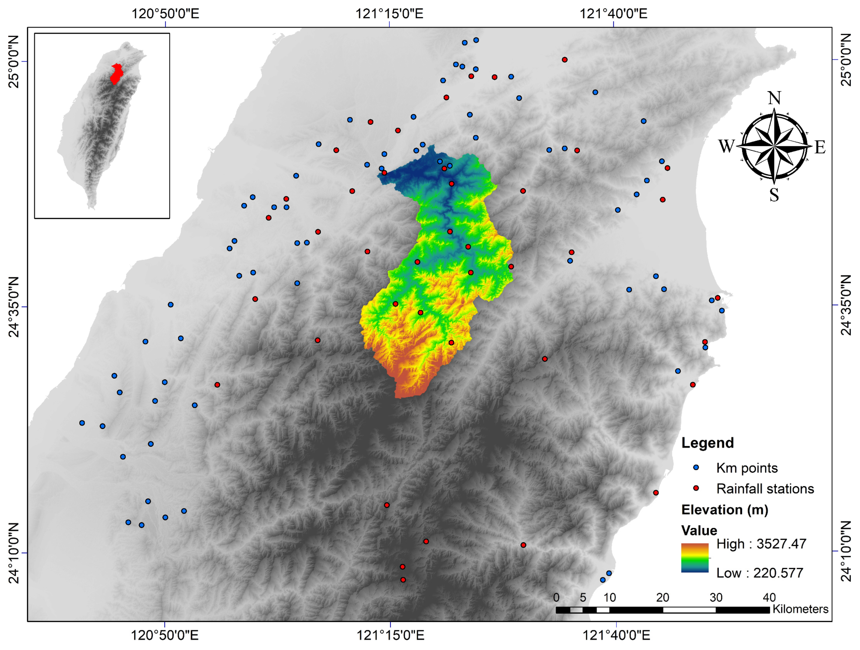
The research area encompassed the watershed of Shihmen Reservoir, one of Taiwan’s most significant reservoirs (Figure 1). The reservoir serves a variety of functions. It is located in the heart of Taiwan and supplies drinking water to important cities such as New Taipei. Additionally, the reservoir serves as an irrigation reservoir, a power generation source, and a flood control reservoir. Regrettably, the reservoir’s watershed is also known to have a high risk of sediment hazard. For instance, the Ronghua Dam, located 27 km upstream of the Shihmen reservoir and capable of holding 12.4 million cubic meters of water, was built in 1983 as a check dam to safeguard the Shihmen reservoir. However, in a short period of time after completion, the Ronghua Dam was nearly completely filled with sediments [5].

The Shihmen Reservoir watershed covers an area of approximately 760 km². The overall topography slopes from south to north (from 3527 to 221 m above the mean sea level, as illustrated in Figure 1), with the reservoir lying on the northern end. The Tahan river is the principal source of water for this reservoir. The watershed receives an annual average of 2400 mm of precipitation due to its mountainous location [22]. Despite the fact that much of the watershed is forested, the area has a long history of human habitation.

To compute soil erosion and deposition using the USPED model, the sediment flow was first computed. We rewrote the equations and their units as follows [12,13,23,24]:

$$T=R_m\times K_m\times L{S}_T\times C\times P$$

(1)

where

• T = sediment flow at transport capacity (Mg∙m/ha/year);
• R_m = rainfall-runoff erosivity factor (MJ∙mm/ha/hr/year);
• K_m = soil erodibility factor (Mg∙hr/MJ/mm);
• C = cover-management factor (dimensionless);
• P = support practice factor (dimensionless);
• LS_T = topographic sediment transport factor (m²/m) and:

$$L{S}_T=U^m\times {\left(sin\beta \right)}^n$$

(2)

where

• U = upslope contributing area per unit width (m²/m);
• Β = angle of the slope;
• m = empirical coefficient; and
• n = empirical coefficient.

Note how similar Equation (1) is to the USLE and RUSLE models. The LS factor (topographic factor) in the USLE and RUSLE models was essentially replaced by the topographic sediment transport factor LS_T. Moreover, USLE and RUSLE simulates soil loss whereas, instead of soil loss, Equation (1) calculates sediment flow at transport capacity. Calculating the divergence of sediment flow is necessary in order to determine soil erosion or deposition:

$$ED=\nabla ·\left(T{S}_0\right)=\frac{\partial \left(Tcos\alpha \right)}{\partial x}+\frac{\partial \left(Tsin\alpha \right)}{\partial y}$$

(3)

where

• ED = soil erosion or deposition (t/ha/year or Mg/ha/year);
• α = aspect of the topography or the direction of flow; and
• s₀ = (cosα, sinα) = unit vector in the steepest slope direction.

When the parameters m = 1 and n = 1 are employed, the sheet erosion mode is dominant. However, when m = 1.6 and n = 1.3 are used, the rill erosion mode is the most prominent. In this study, we adopted the model’s recommended m = 1.3 and n = 1.2 to evaluate a combined occurrence of sheet and rill erosion, as Borrelli et al. [14] did.

The data used in this analysis was gathered from a variety of sources. Liu [25] collected rainfall data from 41 meteorological stations located throughout and around the Shihmen Reservoir watershed, including 31 stations operated by the Central Weather Bureau and ten stations operated by the Northern Region Water Resources Office of the Ministry of Economic Affairs’ Water Resources Agency. The soil erodibility factor was derived from Jhan [26], who scanned and georeferenced Wann and Hwang’s [27] K_m points. Interpolation of the R_m and K_m values was performed using the inverse distance weighting (IDW) method. The locations of the rainfall stations and K_m points are also shown in Figure 1. The topographic sediment transport factor was calculated using a digital elevation model (DEM) produced with Airborne LiDAR, released by the Central Geological Survey (CGS) in 2013. The DEM has a horizontal resolution of 10 m. The cover-management factor C was calculated using data from the Industrial Technology Research Institute’s 2004 national land use survey [28] and Wu et al.’s [29] conversion table between land uses and C factors. Liu [25], Wang [30], and Lo [31] subsequently revised the C factors. Finally, the P factor was assumed to be one, as is customary in the literature when no protection mechanisms are available.

This study followed the procedures indicated on the USPED website [32]. The same findings were found using both GRASS (Geographic Resources Analysis Support System) GIS 7.8 and ArcGIS 10.4.1. However, in both cases, the DEM was not filled and the flowlines and flow accumulation were calculated using the GRASS GIS r.flow and r.watershed modules. GRASS GIS’s flow direction algorithm was implemented using a combined raster–vector technique [33] that is not available in ArcGIS. This component was always computed in GRASS GIS and imported into ArcGIS as needed.

As with USLE-based research, the purpose of this study was to determine the long-term (10–20-plus years) average of soil erosion in the study watershed rather than for a single year or month. Whenever possible, we analyzed obtained data on a yearly average basis. However, the data are not contemporaneous and contemporaneous data were unavailable. This is one possible source of modeling inaccuracy but given the temporal and geographic scope of the investigation, it was unavoidable.

3. Results

Figure 2 illustrates the results of an analysis of the Shihmen Reservoir watershed using USPED. The soil loss and deposition were classified in the same way as Borrelli et al. [14]. On the one hand, there are seven categories of soil erosion: 0–1, 1–3, 3–5, 5–10, 10–20, 20–40, and >40 Mg/ha/year. Soil deposition, on the other hand, is divided into two categories: 0–6 Mg/ha/year and >6 Mg/ha/year. When compared to USLE-based research conducted in the same watershed [5,6], a clear distinction can be detected. Previous research was only able to demonstrate the distribution of soil erosion; however, our study was able to also determine the distribution of deposition. By and large, the northern portion of the watershed, which is adjacent to the reservoir, experiences less soil erosion than the southern portion of the watershed. This corresponds to the forecast made by machine learning models using erosion pin methods [34]. Deposition, on the other hand, is more common around natural depressions, roadways, and riverbanks. 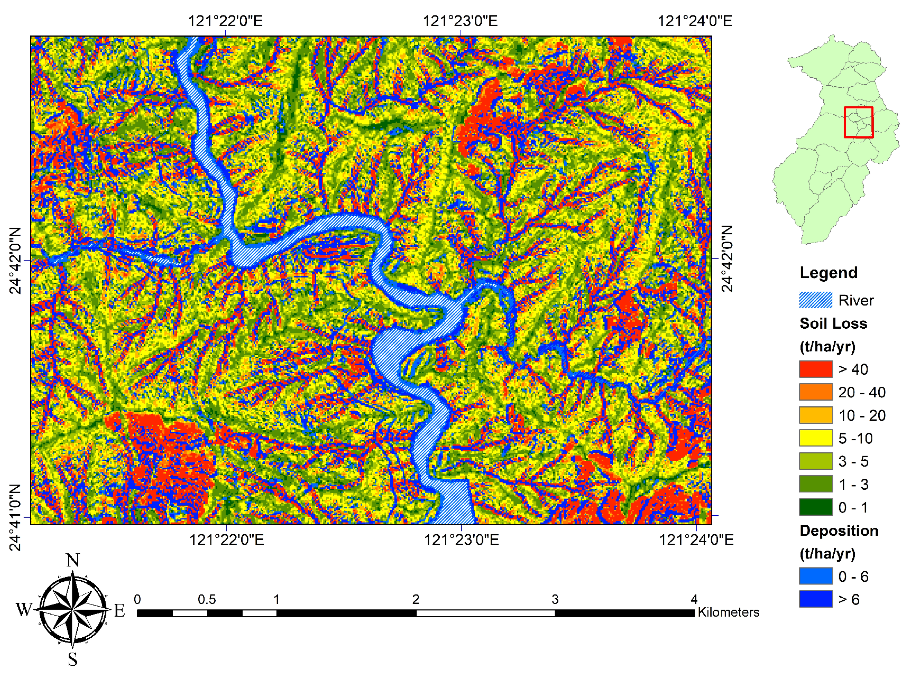Additionally, as illustrated in Figure 2, areas of high soil erosion (>40 Mg/ha/year in red) cluster in multiple locations throughout the watershed. Zooming into the map’s center for example, we can see the spread of soil erosion and deposition more clearly, as illustrated in Figure 3. Erosion hotspots are in red and the relatively stable ground is in green. Additionally, the illustration clearly depicts the distribution of deposition in addition to the distribution of erosion. This is a step forward from USLE-based analysis which calculates and displays only soil erosion. 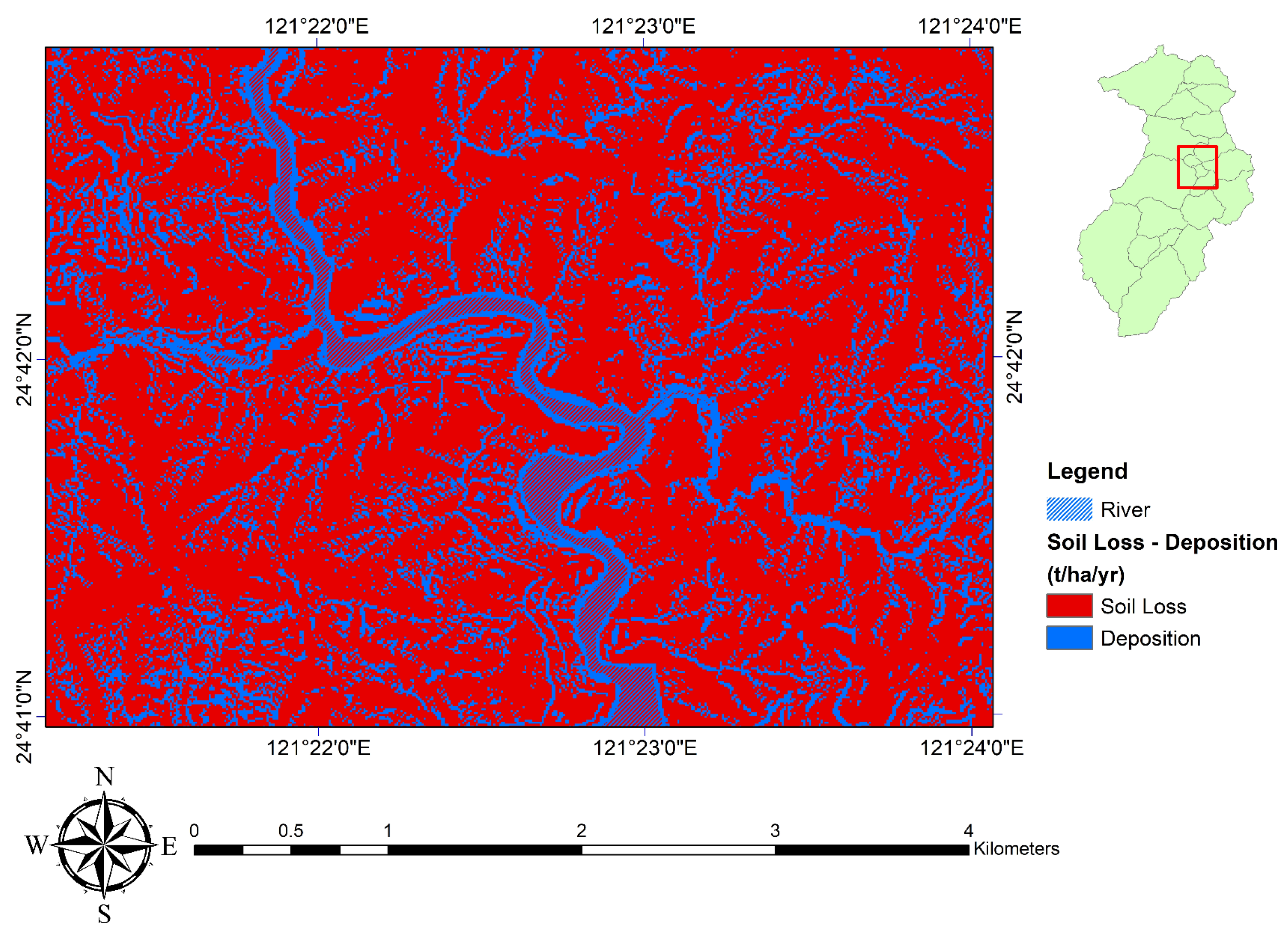Furthermore, when the color scale of the map (Figure 3) is reduced to two hues with red representing soil erosion and blue representing soil deposition, as shown in Figure 4, it is even more clear that soil erosion is more widespread than soil deposition, reflecting the presumed nature of sheet erosion and rill erosion. Also, the distribution of soil deposition is clearly more linear. Additionally, it can be seen that a substantial amount of soil was deposited on both sides of rivers. This is because, in theory, water bodies do not have any exposed soil to erode and are therefore considered areas without soil loss in both the USLE and USPED models. Consequently, the USPED model predicted sediment flow to be nil in the rivers. The abrupt cessation of sediment flow resulted in soil being deposited in areas where water enters into river channels. As a result, sediments accumulated on the riverbanks.

As indicated in

Table 1. Average soil erosion and deposition in the Shihmen Reservoir watershed.

	Total (Mg)	Average of Watershed (Mg/ha/Year)	Area of Occurrence (ha)	% of Total Watershed Area	Average of Occurrence Area (Mg/ha/Year)
Erosion	10,357,271	136.4	60,153	79.2%	172.2
Deposition	10,359,307	136.4	14,582	19.2%	710.4
Net	2036	0.03	-	-	-

, the total soil erosion and soil deposition in the Shihmen Reservoir watershed was approximately equal at $1.04\times {10}^7$ Mg, with soil deposition slightly more than soil loss. The average rate of soil erosion was 136.4 Mg/ha/year while the average rate of soil deposition was also 136.4 Mg/ha/year. However, soil erosion occurred over a greater geographical region (60,153 hectares) than soil deposition (14,582 ha). The phenomenon of soil erosion occurring across a larger area than soil deposition is intriguing. The average rate of soil erosion in the eroded region was 172.2 Mg/ha/year while the average rate of soil deposition in the deposited area was 710.4 Mg/ha/year. Worth noting is that the sum of the eroded and deposited areas was not 100%. The remainder was devoted to rivers and a reservoir.

While this study lacked a method for validating soil deposition, the estimated soil erosion could be compared to in situ data. Between 8 September 2008 and 10 October 2011, the Shihmen Reservoir watershed was instrumented with 550 erosion pins on 55 slopes prone to erosion. On average, soil erosion occurred at a rate of 6.5 mm/year [5]. The erosion depth predicted using the USPED model was 9.7 mm/year assuming that the soil has a bulk density of 1.4 Mg/m³. The result suggested that USPED overestimated soil erosion in this study. However, we conducted the modeling using only the model’s recommended m = 1.3 and n = 1.2 empirical coefficients. The empirical coefficients could be adjusted to account for different relative contributions of rill and inter-rill erosion in the watershed. Alternatively, the coefficients could be tweaked to match the USPED result to the erosion pin measurement. We used the default coefficients solely to demonstrate the capabilities of the USPED model, and the result was fairly satisfactory. Additional coefficient adjustment to achieve unrealistically good agreement between modeling and measurement is pointless for a modeling of this scale and other sources of modeling inaccuracy. As a point of comparison, Harmon et al. [23] discovered that overestimation occurred with a greater margin of error in a North Carolina watershed (1235 m³ vs. 153 m³ of soil erosion). However, Borrelli et al. [14] found that soil erosion in a central Italian watershed was underestimated (2.1 mm/year predicted vs. 3.8 mm/year measured).

3.1. Case Study of Sule Sub-Watershed

Due to the study watershed’s vastness, it is difficult to see the detailed distribution of soil erosion and deposition in Figure 2. As a result, we chose a sub-watershed for additional analysis. During our investigation of this region, we discovered that the Sule sub-watershed is the only one that remains the same regardless of whether the total watershed was divided into 21 or 93 sub-watersheds based on flow accumulation. The Sule sub-watershed also possesses various characteristics and is located around the map’s center as shown in Figure 5. These facts led us to choose it as a case study for further analysis. We utilized it to demonstrate the USPED results in further detail.

The Sule sub-watershed is 406 hectares in size and ranges in height from 474 to 1374 m above the mean sea level. Figure 5 depicts its digital elevation model (DEM). Mountains surround the sub-watershed on both sides and a river flows through the center from south to north. The results generated using the USPED model are depicted in Figure 6. Erosion was most severe on the upper parts of slopes and along the natural depression lines in the terrain. Notice that there are two bridge crossings towards the map’s bottom (southern part).

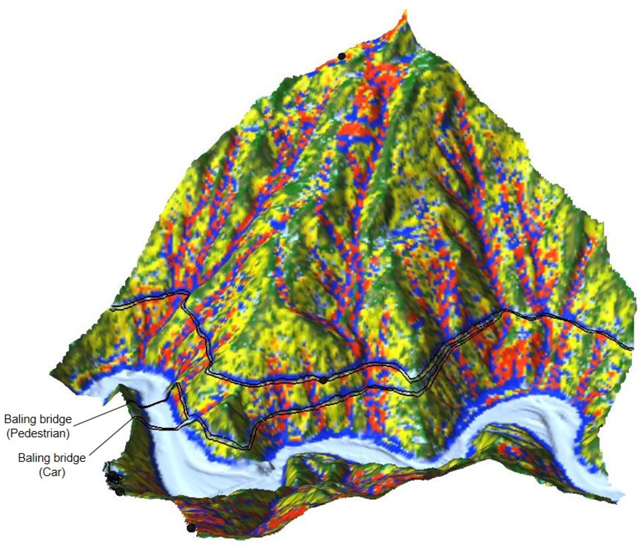
To illustrate how soil erosion and deposition are dispersed across the terrain, we superimposed the soil erosion and deposition map in Figure 6 onto a 3D terrain model and observed the mountain on the west side (Figure 7). We can see that the ridge tops have minimal soil erosion (green) while the elongated low areas between hills and ridges experience concentrated water flow, resulting in significant soil erosion. Along the path leading to the river, soils deposit when the sediment carrying capacities of the flow pathways change. For soils that are not deposited along the way, they are eventually deposited at the river channel’s entry locations, because T = 0 in the river (Equation (1)). This results in the formation of a blue band on both sides of the river.

In addition to the blue bands on the riverbanks, Figure 7 clearly shows two more horizontal blue bands that correspond to two roadways. When sediment flows move down the watershed’s hillside and through the roadways, they deposit soils on the roadways’ upper slopes because of the reduction in sediment carrying capacities. Figure 7 also shows two river crossing bridges connected to the bottom roadway, one for pedestrians and one for automobiles.

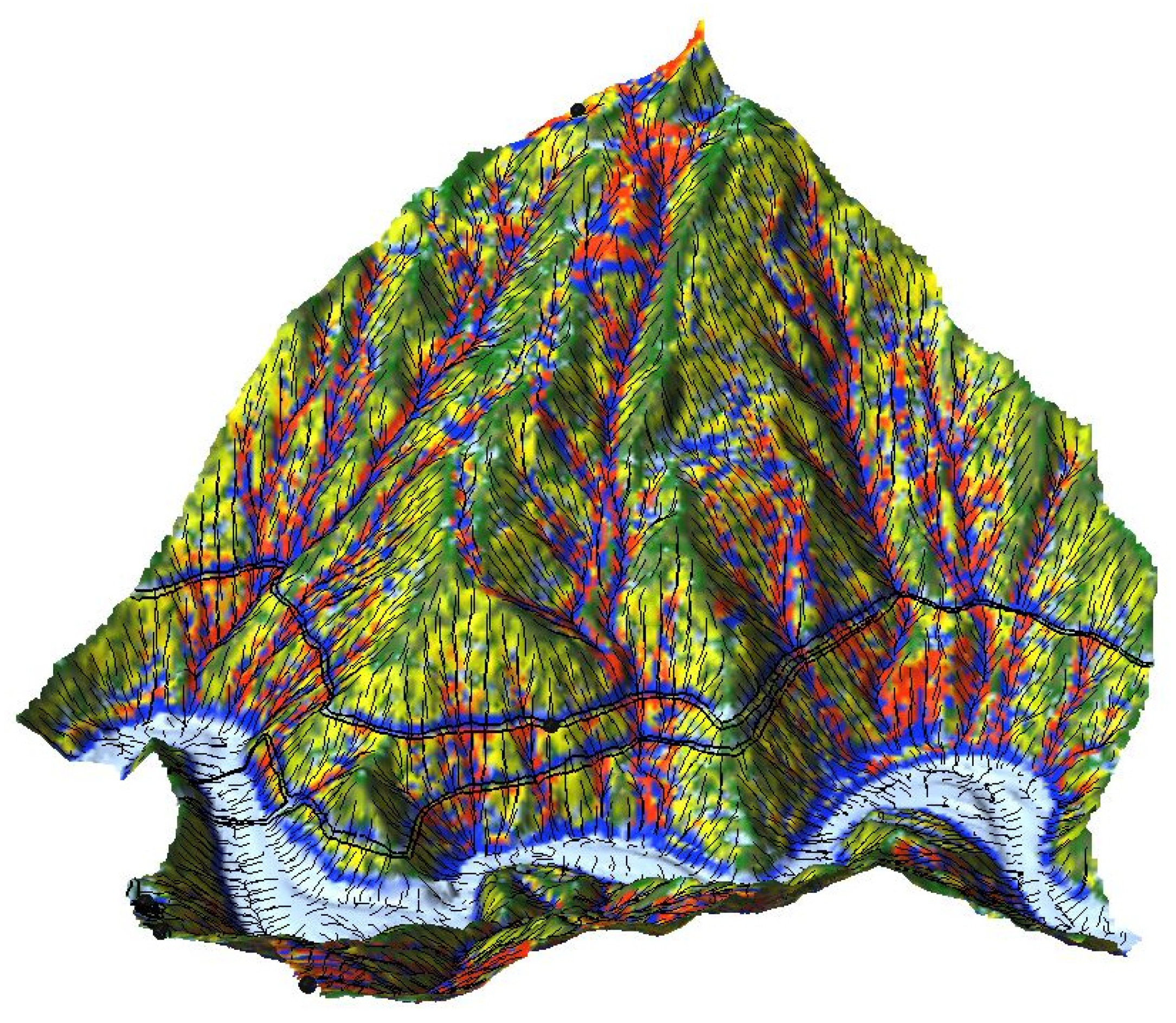
To demonstrate how water flow influences soil erosion and deposition in the area, we further overlaid the flow lines on the soil erosion and deposition map in Figure 8. The flows began at the top of the hill. They converged along natural depression lines following the undulations of the landscape. After that, they flowed through the roadways and into the river. They eroded or deposited soils in the process.

3.2. Factor Comparison for Kala Area

The Kala area, which is located immediately east of the Sule sub-watershed, was chosen for an in-depth examination due to its proximity to the Sule sub-watershed and the anthropogenic activities brought about by settlement. The goal of this example was to explore the effects of erosive factors on soil erosion and deposition and how these factors are linked to human settlement.

The area’s R_m and K_m factors are depicted in Figure 9a,b. The area’s R_m values are predominantly orange and yellow, indicating that they are in the lower range of the Shihmen Reservoir watershed’s rainfall erosivity. Similarly, the K_m values are predominantly yellow and in the lower range of the Shihmen Reservoir watershed’s soil erodibility. R_m and K_m are almost constant in the region at the scale of our modeling, as illustrated in the figures. The LS_T factor is depicted in Figure 9c. The majority of the area had a low LS_T value (red), but as the flows converged, the LS_T factor significantly increased (from yellow to green and eventually blue), attaining maximum values. The distribution of the C factor is depicted in Figure 9d. The values were assigned in accordance with the land use classifications and varied from 0 to 0.25. Due to the relatively constant values of R_m and K_m, the LS_T and C factors were the primary contributors to the observed results. These two factors had a significant effect on how soil erosion and deposition are distributed in the area.

Figure 9e illustrates the computed sediment flow. It exhibits a pattern quite similar to Figure 9c but magnified or diminished by the C factor of Figure 9d. When we computed the divergence of Figure 9e in order to derive the soil erosion and deposition distribution in Figure 9f, an entirely different distribution emerged. Red in Figure 9f denotes erosion while blue denotes deposition. Again, erosion accounted for the great majority of the area whereas deposition accounted for a small percentage.

Figure 9g shows a color rendition of Figure 9f’s soil erosion and deposition distribution. As observed in the figure, relative stable zones (green) occupy a modest area. The majority of the area is shown in orange or red (high erosion). This is due to the area’s anthropogenic activities. As observed in the satellite image (Figure 9h), the USPED model’s high estimates of soil erosion correspond to the local community’s land development and agricultural activities. Additionally, similar to the Sule sub-watershed, the three blue bands in Figure 9g correspond to the rivers visible in the satellite image.

4. Discussion

We used the USPED model to conduct a watershed-scale simulation (760 square kilometers) in this study to estimate the locations of soil erosion and deposition in the watershed. We estimated that the average annual soil erosion for such a large watershed is 136.4 Mg/ha/year. This figure is slightly higher than the earlier USLE results (95.5 Mg/ha/year by Chen et al. [6]; 97.0 Mg/ha/year by Liu et al. [5]; 127.0 Mg/ha/year by Liu [25]; and 110.20 Mg/ha/year by Lo [31]), owing in part to the differences in R_m and C values. However, the primary distinction is that USPED replaces the topographic factor (LS) in USLE with the upslope contributing area and the topographic sediment transport factor (LS_T). Additionally, USPED does not multiply the five erosive factors (Rm, Km, LS, C, P) when calculating soil erosion; rather, it multiplies the five erosive factors when calculating sediment flow. Soil erosion or deposition occurs when the divergence of sediment flow changes. While this investigation did not validate soil deposition, we discovered that USPED’s average soil erosion is greater than the erosion pin measurement in the research region (9.7 vs. 6.5 mm/year). The inaccuracy, however, is not as large as that observed in Harmon et al. [23] who considered a much smaller watershed. Although the estimate of USPED was greater than the erosion pin measurement and the previous USLE estimates, the USPED model was able to depict the sediment distribution inside the watershed and gave modeling results previously unavailable for sediment hazard prevention.

Moreover, two empirical coefficients, m and n, regulate the USPED model. We used the model recommended m = 1.3 and n = 1.2 for this study as Borrelli et al. [14] did. For prevailing rill erosion, the USPED recommends m = 1.6, n = 1.3, but for prevailing sheet erosion, the USPED recommends m = n = 1. For comparison, we also conducted a simulation for the Shihmen Reservoir watershed with m = n = 1 and discovered that the average annual rate of soil erosion and deposition for the entire watershed was 10.4 Mg/ha/year, which was less than the erosion pin measurement. However, if m = 1.6 and n = 1.3 were utilized, the average soil erosion would be 2453.6 Mg/ha/year and the average soil deposition would be 2464.1 Mg/ha/year, which was bigger than the erosion pin measurement. As can be observed, the modeling results vary significantly depending on the values of m and n. On the basis of these results, it is possible to adjust the m and n parameters to obtain their optimal values that fit the erosion pin measurement. However, this may not be meaningful given the model’s complexity and other causes of inaccuracy.

Because water bodies such as rivers and reservoirs have a zero C factor, their sediment flow is also zero in the USPED model. When surface water joins rivers, the sediment carrying capacity abruptly decreases to zero, causing sediments to settle at the river’s entry points (riverbanks). As a result, the entire Shihmen Reservoir watershed is a self-contained area in the simulation. Sediments were not allowed to exit the watershed. However, the total soil deposition calculated in this study was slightly greater than the total soil erosion (difference = 0.02%). It is possible that this is due to USPED’s model limitations or rounding errors in the GIS computation.

Figure 10 shows the percentage of total sediments deposited as a function of the distance from the watershed’s rivers. The figure and associated computation show that 3.4% of all sediments were deposited within 10 m (which is the grid cell size) of the rivers. These are the sediments that should have entered the rivers but instead were deposited directly next to them due to the model assumption. Figure 10 clearly shows that when the buffer size grows, the percentage of sediments deposited in the buffer zone next to the rivers increases almost linearly. The buffer distance is crucial because if there is a landslide of sediments when the next typhoon, torrential rain, or earthquake occurs, the distance determines whether the sediments will be swept into the rivers or not. The average runout distance of landslides, according to the literature, depends on many factors. For example, Prochaska et al. [35] compiled a table of 23 events with runout distances ranging from 142 to 785 m, with the exception of a 3178 m runout. Xu et al. [36] also demonstrated in a table of 53 shallow loess landslide incidents that the runout distance varies between 25 and 621 m. These two ranges have midpoints of 464 and 323 m, respectively. The USPED model indicated that 12.6% of sediments in the Shihmen Reservoir watershed was inside a 200 m buffer and 26.3% percent was within a 500 m buffer zone.

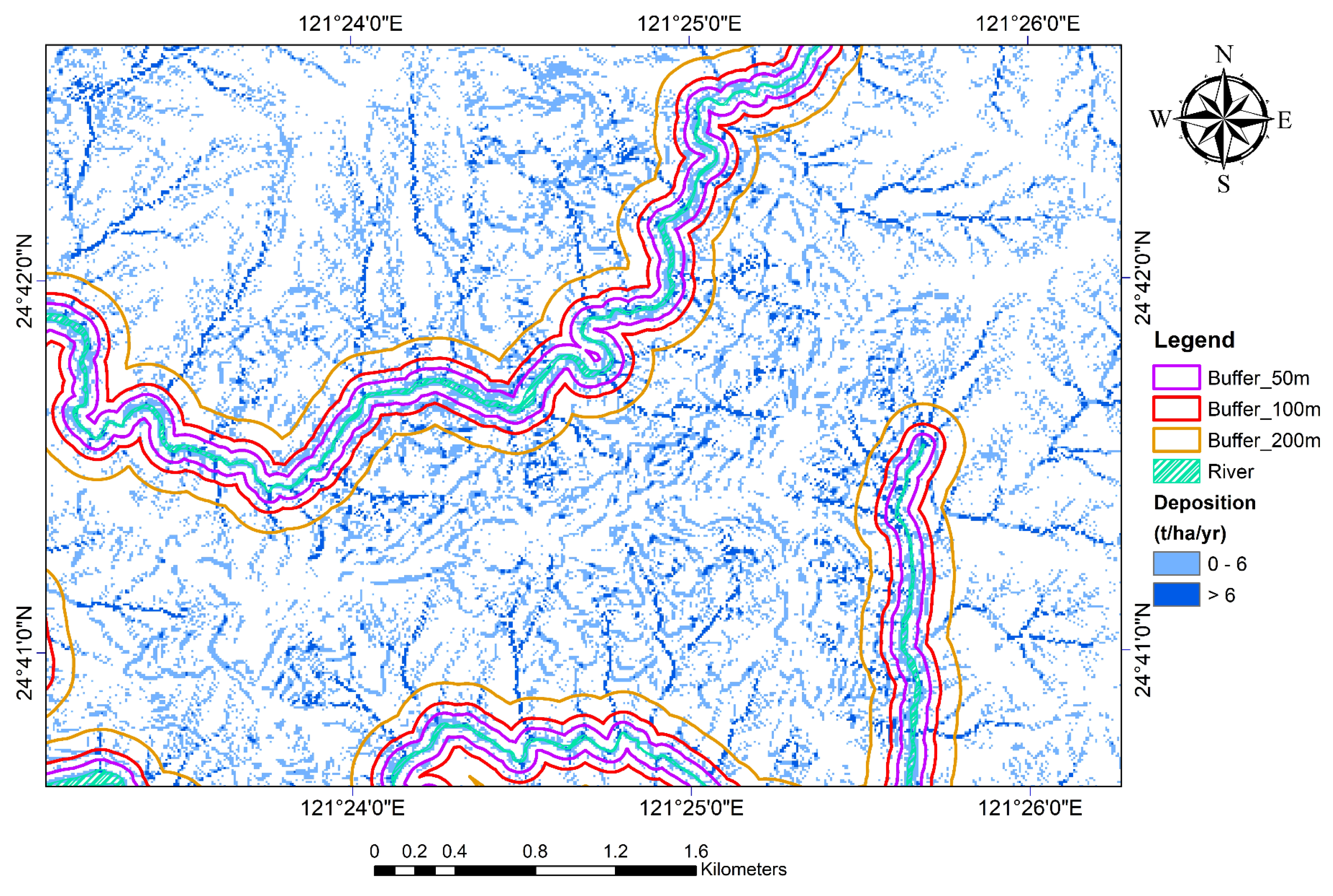
Additionally, Figure 11 depicts the soil deposition map of Kala area with 50, 100, and 200 m buffers around all of the rivers to illustrate the area’s sediment distribution. As with prior figures, soil deposition is classified into two categories: 0–6 Mg/ha/year and >6 Mg/ha/year. However, soil erosion was omitted from the figure to prevent cluttering it. As illustrated in the figure, the sediment distribution was influenced by surface runoff and intersected the rivers at almost a straight angle. This explains why the percentage of sediments deposited in the buffer zone had a linear relationship.

The USPED model assumes that soil detachment significantly surpasses the ability of overland flow to transfer sediments. As a result, the sediment flow rate is equal to the sediment transport capacity. As such, USPED is a transport-capacity-limited model. Soil erosion occurs when the divergence of sediment flow is positive, causing the carrying capacity of sediment flow to grow while the soil detachment increases in order to fulfill the capacity. When the divergence is negative, it indicates soil deposition [37,38].

The USPED modeling results were adequately demonstrated in the 406 hectare Sule sub-watershed where the soil is mostly stable due to good vegetation. The topography contains many undulating ridges and draws, as shown in the 3D view (Figure 7). As a result, concentrated surface runoff was largely responsible for soil erosion and deposition, which occurs primarily along slope drainage lines. Many of these runoffs are even hidden by lush vegetation, making them unnoticeable from the air.

Finally, according to Li’s [39] literature review, the average rate of gully erosion in the Shihmen Reservoir watershed was 6.9 Mg/ha/year whereas the average amount of soil displaced by landslides was 46.0 Mg/ha/year. The Shihmen reservoir’s average siltation rate between 2011 and 2015 was 71.2 Mg/ha/year. Thus, an estimate of the watershed’s sediment delivery ratio based on the USPED model was 71.2/189.3 = 0.38.

5. Conclusions

We conducted a watershed-scale simulation (760 square kilometers) in this study using the USPED model to determine the locations of soil erosion and deposition in the watershed. Additionally, we selected the Sule sub-watershed and the Kala area as examples to illustrate the pattern of soil erosion and deposition and their relationship to rivers, roadways, and anthropogenic activity. Even though the entire watershed depicted in this study is enormous, when we focused in on the two cases, we achieved good and reasonable results that fit the local conditions. In comparison to prior USLE- and RUSLE-based soil erosion modeling in the same research area, our USPED modeling is unique in that it additionally included both the amount and distribution of soil deposition. This successful implementation of USPED in Taiwan establishes a new modeling alternative in addition to the widely used USLE and RUSLE models. The results can be used to guide the future location selection of erosion pins in the research area, ensuring that they cover both erosion and deposition zones. The new erosion pin readings can then be utilized to evaluate the model output, increasing our ability to model sediment movement and avoid sediment hazards. Although this was a regional study, it compensates for the USPED model’s limited geographic reach and provides another application example for a comprehensive assessment of the USPED model’s effectiveness as a soil erosion modeling tool.