Abstract
Environmental pollution has attracted growing government attention. We employ a series of panel data regression models to measure and analyze the impact of environmental attention of 284 prefecture-level municipal governments on ambient pollution in China. The results show that: (1) The improvement of government environmental attention can curb ambient pollution. (2) The impact of government environmental attention on ambient pollution is heterogeneous in the difference of regional and local environmental pollution severity. (3) Government environmental attention inhibits ambient pollution through green development and industrial upgrading. The conclusions of this paper provide evidence and implications for environmental regulation in developing countries and cities.
1. Introduction
1.1. Motivation
Since the 1960s, the environmental problems caused by large-scale industrial production have attracted widespread attention, and ambient pollution has become one of the main focuses of the public in many countries. The harm of ambient pollution such as PM2.5 to human health has been confirmed, mainly causing respiratory obstruction or inflammation by assisting pathogenic microorganisms, chemical pollutants, and oil fumes [1,2]. In order to cope with the problematic ambient pollution situation, governments of various countries and regions have continuously strengthened their attention to the environment and issued relevant regulations.
In the past few decades, the U.S. government has established a number of environmental protection policies through the Environment Protection Agency (EPA) to reduce and control urban pollution and has achieved some results. The 2020 EPA report showed that, from 1970 to 2019, the U.S. GDP increased by 285%, population by 60%, miles driven by 195%, energy consumption by 48%, and carbon dioxide (CO2) emissions increased by 25%, but the ambient pollution decreased by 77%. All primary air pollutants levels have decreased significantly over the past few decades. According to the U.S. EPA’s National Air Quality Summary, from 1980 to 2019, carbon monoxide emissions decreased by 75%, lead emissions decreased by 99%, nitrogen oxides (NOX) emissions decreased by 68%, volatilization emissions of sexual organic compounds (VOCs) were reduced by 59%, PM10 emissions by 63%, PM2.5 emissions by more than 36%, and sulfur dioxide emissions by 92%. The overall air quality improvement in the United States is mainly due to the continuous innovation of industrial production technology and the deindustrialized urban development model, but despite this, many urban populations are still affected by ambient pollution. The U.S. Environmental Protection Agency reported that, in 2019, roughly 81.9 million people, or 25 percent of the U.S. population, lived in areas with concentrations of at least one air pollutant that exceeded federal standards. By pollutant categorization, 2.8 million, 15.4 million, and 22.5 million people live in areas where sulfur dioxide, PM2.5, and PM10 exceed the standard.
On 12 May 2021, the European Commission issued the “EU Action Plan: Towards Zero Pollution for Air, Water and Soil”, which aims to reduce air, water, and soil pollution to a level that is no longer harmful to human health and natural ecosystems by 2050. The action plan is a key outcome of the European Green deal. A series of key action plans to achieve zero pollution by 2050 are set.
Since the reform and opening up, China’s economy has snowballed [3], but the natural ecological environment has been severely damaged. The increasingly severe environmental pollution problem has endangered the average production and life of the public and the sustainable development of the economy. PM2.5 is one of the primary air pollutants in China, and it is also one of the air pollutants with the most consistent results and the most apparent health hazards in long-term exposure studies [4,5]. In most areas of China, the concentration of PM2.5 has been relatively high. From 2014 to 2016, 95%, 87%, and 81% of the population were exposed to the environment, exceeding the national standard of 35 μg/m³. Almost no one’s exposure environment can reach the 10 μg/m³ recommended by the WHO [6]. Studies have demonstrated that long-term exposure to high PM2.5 concentrations increases the morbidity and mortality of numerous diseases, particularly in low- and middle-income communities [7]. The Global Burden of Disease (GBD) research report of 2015 showed that PM2.5 has become the fifth-leading cause of death globally. In 2015, the global death toll attributable to PM2.5 exposure was 4.2 million, of which China accounted for 1.1 million, which was more than a quarter. The mortality rate in China attributable to PM2.5 pollution is 84.3 per 100,000 people, which is more than four times that of the United States (18.5 per 100,000 people) [8].
Given the grim situation of ambient pollution, the Chinese government has also made many efforts. In September 2013, the “Action Plan for Air pollution Prevention and Control” issued by the State Council proposed accelerating the construction of desulfurization and other transformation projects in major industries. In September 2014, the National Development and Reform Commission and other agencies released the “Notice on Adjusting the Collection Standard of Sewage Charges and Other Related Issues”, which doubled the collection standard of sewage charges per pollution equivalent of waste gas and sewage, requiring to strengthen the environmental law enforcement and inspection of the collection of sewage charges. In December 2015, the Ministry of Environmental Protection and other departments issued the “Work Plan for the Full Implementation of Ultra-low Emission and Energy Saving Transformation of Coal-fired Power Plants”, mandating that coal-fired power facilities in the east, middle, and west achieve ultra-low emissions by the end of 2017, 2018, and 2020, respectively. The emission concentrations of smoke, SO2, and NOx must not exceed 10 mg/m3, 35 mg/m3, and 50 mg/m3, respectively, under the condition of a 6% reference oxygen content. Coal-fired units achieve average dust removal, desulfurization, and denitration rates of more than 99.95%, 98%, and 85%, respectively. In December 2016, the State Council issued “The Comprehensive Work Plan for Energy Conservation and Emission Reduction” in the 13th “Five-Year Plan”, which significantly improved the goal of ambient pollution control. In September 2017, the Ministry of Environmental Protection proposed the “Prevention and Control of Volatile Organic Compounds Pollution” in the 13th “Five-Year Plan” to focus on promoting the prevention and control of VOC pollution from critical industries such as petrochemical; chemical; packaging and printing; industrial coating; and other traffic sources, such as motor vehicles and oil storage, transportation, and marketing. In July 2018, the State Council issued “The Three-year Action Plan for Winning the Blue Sky Defense War”, defining the overall idea, primary objectives, main tasks, safeguard measures, and planning process of ambient pollution prevention and control. In May 2019, the Ministry of Ecological Environment and other departments jointly issued “The Opinions on Promoting the Implementation of Ultra-low Emission in the Iron and Steel Industry”, which outlined the general goal of fostering ultra-low emissions in the steel sector. The 2020 Central Economic Work Conference stated that China should fight hard against pollution; stick to one direction and strength; emphasize precise pollution control, scientific pollution control, and pollution control according to law; and promote continuous improvement of the ecological environment.
With the continuous deterioration of the environment, the local government inevitably needs to assume greater social responsibility, and the relationship between the local government’s environmental attention and ambient pollution from the meso-perspective is the value of the investigation. In this context, we can raise some questions: Does the government’s environmental attention directly affect ambient pollution? What are the differences in the role of government environmental attention on ambient pollution among different subjects? How does the government’s environmental attention affect ambient pollution? We must use appropriate measurement methods and theories to analyze these problems. Figure 1 shows the logical structure diagram of this study.
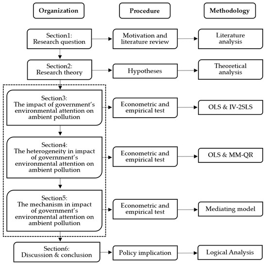
Figure 1.
The logical framework.
1.2. Literature Review
It is generally accepted that government actions have impacts on the environment [9]. Wang et al. introduced environmental and carbon levies to determine the appropriate power mix [10]. To prevent the “peak” impact of polluted weather, Yang et al. recommend promoting individual adaptive actions [11]. According to research, the Chinese government should invest more effort than only enacting environmental legislation [12]. Hao et al. utilized panel data from 30 provinces in China from 1998 to 2016 to evaluate the influence of FDI and technological innovation on environmental pollution [13]. Although the influence of environmental regulations on happiness has been debated, the present research has neglected it [14]. From the standpoint of environmental pollution, Wu et al. suggested a set of policy implications for reducing criminal activities in China [15]. Gao et al. addressed the effects of short- and long-term pollution exposure [16]. The importance of another study highlights the impact of coronavirus disease on urban ambient pollution [17]. Carbon financial market, carbon tax, carbon pricing, and economic uncertainty are some important factors affecting pollution and closely related to government behavior [18,19,20,21,22,23,24,25].
Ambient pollution has been extensively studied in the past. Adamczyk et al. presented a wide range of activities aimed at the reduction of the environmental impact of the emissions of pollutants from individual heat sources, the so-called low emission [26]. Liao et al. investigated UPM pollution to analyze its source, composition, and distribution characteristics of UPM in ambient air [27]. Świerszcz et al. considered the implications of geothermal energy as an alternative source for the counteracting of low emissions as part of the ecological security strategy [28]. Loyeva et al. presented an algorithm of a complicated statistical analysis of atmospheric air pollution over certain urban territories based on the methods of a multivariate statistical analysis and a statistical decisions theory [29]. There have been many other influential studies [30,31,32].
PM2.5 is one of the leading indicators used to measure ambient pollution, and the relevant research has been relatively mature [33]. To interpret globally scattered PM2.5 mass and composition measurements from the Surface Particulate Matter Network (SPARTAN) [34], Weagle et al. utilized the GEOS-Chem simulation by satellite-based estimations of PM2.5. Liu et al. employed a random forest-based geostatistical (regression kriging) technique to improve one of the most widely used satellite-derived, gridded PM2.5 datasets with a finer spatial resolution (0.01°) and improved accuracy [35]. In order to predict the PM2.5 levels in the North China Plain, Huang et al. created a high-performance machine learning model directly at the monthly level [36]. Shi et al. used standard deviation ellipse and trend analysis to examine the regional and temporal features of PM2.5 in South and Southeast Asia, based on a long-term series of satellite-retrieved PM2.5 concentrations [37]. By integrating a chemical transport model with a complete emission inventory, Zhang et al. calculated the air quality and health benefits of certain clean air activities [38]. With hourly ozone and PM2.5 readings from 106 locations in the North China Plain from 2013 to 2018, Li et al. provided observational evidence for this impact [39]. Stafoggia et al. used random forest to predict the daily PM10, fine, and coarse particles at 1-km2 grid [40]. Choi et al. investigated source contributions to PM2.5 in South Korea under various meteorological conditions, using a suite of extensive observations of PM2.5 and its precursors’ concentrations collected during the international Korea–US cooperative air quality field study in Korea in May to June 2016 [41].
There have been few direct studies on the impact of government actions on ambient pollution in the past. The CSN database was used to explore the long-term variants of pollution sources to PM2.5 organic carbon (OC) in Central Los Angeles and Riverside from 2005 to 2015, during which a few federal and state PM-based legislations were taken to minimize the tailpipe emissions in the region [42]. The research purposed by Park et al. was to investigate the impacts of PM2.5 on domestic and Chinese components identified in the Korean government’s policy [43]. The research of Zhang et al. applied the CMAQ model to analyze the effectiveness of pollution regulations to give data-driven assistance to policy decisions, which are becoming more crucial [44]. Wang et al. employed long-term reliable data to explore the variance of air pollutants in China, in which the Chinese government has made substantial efforts to decrease the emission levels in polluted locations [45]. In addition, the research on government actions such as limiting vehicle emissions, afforestation projects, and increasing financial expenditure on energy conservation and environmental protection has also obtained meaningful conclusions [18,46,47].
1.3. Contribution
Compared with previous studies, the innovations and contributions of this paper are as follows. (1) We collect the annual government work reports of more than 200 prefecture-level cities in China and use text analysis technology to measure the data of municipal government environmental attention, filling the gaps in the government environmental regulation research from a meso-perspective. Compared with previous studies, which are keen to use environmental tax to represent the intensity of the environmental regulation, this paper directly uses the government’s environmental attention, which can more truly reflect the local government’s subjective willingness to regulate the environment. (2) Compared with previous studies, the sample size of this paper is larger, and the period is more extended, which can get more accurate and practical conclusions. (3) This study makes full use of the measurement methods to build targeted measurement models for different problems. Firstly, the fixed effect panel model and 2SLS method are used for estimations, confirming the inhibitory effect of urban government environmental attention on ambient pollution. Secondly, the mediating effect model is applied to verify the path role of the green development effect and industrial upgrading effect in the impact. Finally, the heterogeneity of urban government environmental attention on ambient pollution is analyzed using subsample regression and the MM-QR method.
As the largest developing country in the world, China has sufficient urban samples for empirical analysis. The relevant conclusions can provide practical experience for governments worldwide to formulate environmental protection policies. Furthermore, China’s economic development is seriously unevenly distributed, and the level of economic development is gradually declining from the eastern coast to the western inland. Therefore, the empirical results of Eastern, Central, and Western China can provide targeted experiences for developed countries, middle-level countries, and backwards countries, respectively.
2. Research Design
2.1. Hypotheses
The actual effect of government environmental regulation can be considered from two perspectives. On the one hand, government environmental regulation is difficult to curb pollution. China’s investment in environmental pollution control has accounted for only about 1.5% of the GDP in many years. The Chinese government mainly promotes enterprises to reduce pollution by implementing a sewage charge system. However, many enterprises prefer to pay sewage charges rather than reduce emissions [48]. The government has also increased financial subsidies to reduce the cost of pollution reduction of enterprises, and even the phenomenon of subsidy funds exceeding the amount of pollutant discharge fees has caused many enterprises to take the opportunity to obtain state subsidy funds without increasing their investment in pollution control. On the other hand, environmental pollution will be effectively controlled with the growing investment in pollution control and the increasingly stringent environmental regulations. Local governments rely on a solid economic foundation to establish strict and perfect environmental management laws and regulations. At the same time, the public has gradually developed a good awareness of environmental protection and green behavior habits, which is conducive to stimulating the motivation of enterprises to reduce pollution. As the economy enters the stage of low-speed growth, the marginal rate of return of social capital is decreasing, reducing the opportunity costs of pollution control investments and conducive to improving the investment level of pollution control. Generally, urban government regulation can alleviate local ambient pollution in China, where the government has a strong control ability. Accordingly, we propose the following hypothesis:
Hypothesis 1 (H1).
Government environmental attention can inhibit regional ambient pollution.
There must be differences in the willingness and ability of governments to control environmental pollution among different cities. Many variables influence the local government environmental control and the degree of local environmental pollution, including the internal and external environment, location, policy strategy, and infrastructure, in the area. Therefore, there are significant differences in the core elements between different cities. From the geographical location, Eastern China has several important developed urban circles with convenient foreign exchanges. It is China’s most economically advanced area, with highly developed industry, severe ambient pollution, and more flexible government policies. The central and western regions have rugged terrain and relatively backwards transportation development. They are still in a driven role in development planning. The industrial intensity is low, and local governments are more eager for development. They have different attitudes towards environmental problems. In terms of the degree of local environmental pollution, the heavily polluted area itself has a larger amount of pollution sources: a large number of heavily polluting enterprises and populations. In the overall planning of the central government, heavily polluted areas are also under greater pressure from higher authorities. Sometimes, environmental problems are directly linked to the assessment of officials. The environmental protection pressure and difficulty of more heavily polluted cities are higher. Accordingly, we propose the following hypothesis:
Hypothesis 2 (H2).
The heterogeneity of the impact of government environmental attention on ambient pollution is reflected in regional differences and local ambient pollution degree.
Intuitively, the fundamental driving force for reducing ambient pollution comes from reducing pollution emissions from the production sector. Although China is the second-largest economy globally, its per capita economic level still belongs to developing countries. It is unrealistic to require China to give up its development for environmental problems. For the region’s economic development, local governments will not choose to give up industry directly. Improving green production efficiency and industrial structure is the best choice in reality. Environmental laws and regulations mainly reduce pollution by limiting the polluting production factors or the production of commodities. They can also encourage enterprises to invest in pollution control and reduce pollution emissions per unit output to reduce the pollution level, improving green production efficiency. In addition, heavy polluting enterprises are densely distributed in areas with early industrial development, causing tremendous pressure on the local environment. The local government also requires explicitly polluting enterprises to transform or move out, which will be replaced by greener and environmentally friendly industries; that is, using industrial upgrading to reduce pollution. Accordingly, we propose the following hypothesis:
Hypothesis 3 (H3).
Government environmental attention can restrain ambient pollution through green development effect and industrial upgrading effect.
2.2. Model
The first step is benchmark regression. We employ a fixed effect panel regression model to analyze the direct impact of China’s urban government environmental attention on ambient pollution. The model setting is as follows:
where represents a city’s serial number; is the year; represents the dependent variable ambient pollution, i.e., PM2.5 concentration; is the independent variable, i.e., government’s environmental attention; are the covariates, including economic development level, regional urbanization level, upgrading of industrial structure, openness, degree of marketization, population density, transportation development level, and development level of posts; stands for the individual fixed effect; is the error term; and describes the direct impact of the government’s environmental attention on ambient pollution, which is the chief factor in this paper.
The second step is to set the instrumental variable method [49]. This research employs 2SLS to design the model in order to better quantify the influence of on :
Formula (2) is the first stage of 2SLS, and the form of the second stage is the same as Formula (1). is the with a lag period. According to the general practice, endogenous variables with one lag period can meet the correlation assumption and the exogenous assumption of effective instrumental variables.
The third step is for the quantile regression. For verifying Hypothesis 2, we need to further analyze it based on benchmark regression. For regional differences, we can divide samples. However, quantile regression is needed to analyze the heterogeneity based on the difference of the local environmental pollution degree measured with the following formula:
is the quantile of ambient pollution degree, and is the quantile estimation coefficient of the influence of government’s environmental attention on ambient pollution.
The weighted average of the absolute value of the residual, which is not easily impacted by extreme values, is used as the objective function of minimization in the quantile regression initially described by Koenker and Bassett [50]. The fixed effect panel quantile regression with adjustment effect was later introduced by Koenker [51]. Prior quantile analyses believed that a single influence only created a parallel (position) shift in the response variable distribution without changing the whole distribution [51,52]. To put it another way, it ignored unobserved individual heterogeneity. This research uses a novel Minimization Quantile Regression (MM-QR) approach to explore the heterogeneous influence of the government’s environmental attention on PM2.5 in order to tackle this challenge [53]. In estimating panel data models with individual effects and avoiding endogenous difficulties, MM-QR technology provides benefits [54].
The fourth step is the mechanism test. The above theoretical mechanism analysis shows that green development and industrial upgrading are two main mechanisms for the government’s environmental attention to affect ambient pollution. In order to verify these mechanisms, this paper uses the mediating effect model based on the stepwise regression method for empirical research:
where represent the two mediating variables, including urban ecological efficiency () and upgrading of industrial structure (), means the same as it is in Formula (1), measures the impact of the government’s environmental attention on the mediating variable, measures the direct impact outside the mechanism approach, and means the impact of mediating variables on the ambient pollution. In addition, this paper also uses the Sobel test to verify the mediating effect.
3. Data Preprocessing
3.1. Measurement
For the dependent variable, the PM2.5 concentration data () come from the relevant data published by the Socio-Economic Data and Application Center (SEDAC) of Columbia University [55], which is based on the Aerosol Optical Thickness (AOD) measured by the Moderate-resolution Imaging Spectroradiometer (MODIS), Multi-Angle Imaging Spectrometer (MISR), and Sea-viewing Wide Field-of-view Sensor (SeaWiFS) on NASA satellites. The global PM2.5 grid data formed after the transformation of the geochemical transfer model (GEOS-Chem model) and the prediction and adjustment of the Geographically Weighted Regression model (GWR) further take the vector boundary of China’s municipal administrative divisions as the mask and uses the spatial analyst tool in ArcGIS software to count and extract the grid data, so as to obtain the PM2.5 concentration data at the municipal level from 2008 to 2018.
For the independent variable, the measurement of government environmental attention () data refers to the research of Chen et al. [56]. The first step is to extract keywords related to environmental protection from multiple environmental policy reports and words, including environmental protection, environmental protection, green development, new energy, haze, haze control, pollution, energy consumption, pollution control, emission reduction, sewage discharge, ecological environment, ecological protection, ecological damage, water ecology, low carbon, sulfur dioxide, carbon dioxide, PM10, PM2.5, chemical oxygen demand, COD, scattered pollution, discharge, air, water environment, water safety, water quality, clear water, black odor, sewage, waste gas, waste residue, environmental violation, environmental crime, environmental case, environmental punishment, environmental treatment, environmental quality, blue sky, coal combustion, greening, dust, tail gas, and VOCs.
Secondly, we collect the annual government work reports of 284 prefecture-level cities in China during the investigation period. Then, the proportion of statements containing environmental protection keywords in the full text is analyzed. Finally, we use text analysis to measure the proportion of sentences related to environmental protection, which is multiplied by 100 to get the government’s environmental attention of prefecture-level cities in China.
Mediating variables include urban ecological efficiency () and upgrading of the industrial structure (). Urban ecological efficiency is measured by the super-efficient SBM-GML model in data envelopment analysis (DEA), according to the research of Su et al. [57,58]. DEA is one of the most popular methods to measure efficiency [33,59,60]. We take capital, labor, construction, and energy as the four major input indicators; GDP is the desirable output indicator; wastewater, waste gas, and smoke as the three undesirable output indicators. For the indicator of industrial structure upgrading, we adopt the common practice, taking the proportion of the total output value of the secondary industry and the tertiary industry in the urban GDP.
This paper selects seven main control variables related to the urban economy and environment. They are the logarithm of each city’s per capita GDP (); urbanization level (), which is the fraction of each city’s population living in the municipal area [61]; openness (), the city’s real foreign investment share of GDP; marketization (), which is the fraction of private and individual employment in the whole population; the logarithm of the population density () of each city; transportation (), the logarithm of total urban passenger volume divided by total urban population; and postal development level (), expressed as a logarithm of the revenue from postal business divided by entire population. The data of the control variables are from the China Urban Statistical Yearbooks, and missing values are interpolated using the changing trend.
3.2. Statistics
Table 1 reports descriptive statistics for all variables in this paper. In order to reflect the differences among cities in different regions, the descriptive statistics of eastern, central, and western cities are displayed, respectively.

Table 1.
Descriptive statistics.
It can be found that the intensity of ambient pollution in the eastern region is high, followed by the central part, and the degree of ambient pollution in the western region is relatively weak. PM2.5 is the main cause of weather haze. It is generally believed that if the concentration of PM2.5 exceeds 35 μg/m³, the environment is not good. The WHO has pointed out that, when the average annual concentration of PM2.5 reaches 35 μg/m³, the risk of human death is about 15% higher than that of 10 μg/m³. It can be seen that ambient pollution in Eastern and Central Chinese cities has been relatively severe.
In terms of the government’s environmental attention, eastern cities pay the greatest attention, followed by western cities, and central city governments pay the lowest attention to environmental protection. However, there is little difference in government environmental attention among different regions.
4. Empirical Results
4.1. Parameter Estimation
According to the setting of Formula (1), we first briefly analyze the direct impact of China’s urban government’s environmental attention on ambient pollution. Table 2 shows the results of the benchmark regression. Column (1) represents the ordinary OLS regression results of and , and Column (2) considers the seven control variables in this paper based on ordinary OLS. Column (3) displays the regression results of the panel fixed effect; that is, the fixed effect of urban individuals is considered based on Column (2).
Table 2.
Estimation results for the benchmark regression.
According to Table 2, it can be seen that the government’s environmental attention significantly reduces ambient pollution. In Column (1), the PM2.5 concentration decreases by 0.134 μg/m³ for each percentage point increase in the government’s environmental attention. According to the results in Column (3), the PM2.5 concentration decreases by 0.164 μg/m³ for each percentage point increase in the government’s environmental attention. N, FE, and R2 stand for the number of samples, fixed effect, and goodness of fit, respectively.
When directly assessing the influence of government environmental attention on ambient pollution, the foregoing analysis suggests that the endogeneity between fundamental variables may be neglected. To study the influence more quantitatively, we use the 2SLS estimate technique in conjunction with Formulas (1) and (2), and the findings are displayed in Table 3.
Table 3.
Estimation results for the 2SLS.
After considering the instrumental variables, the government’s environmental attention still has a significant inhibitory effect on ambient pollution. Column (1) shows the first stage regression results. Firstly, the correlation between and is proven to be significant. The regression results indicate that there is no problem with weak instrumental variables. According to Column (2), it can be seen that the government’s environmental attention still has an inhibitory effect on the ambient pollution, but this impact degree is not the same as that in the benchmark analysis. After eliminating the endogenous problems of the core variables, the government’s environmental attention even has a more significant inhibitory effect on ambient pollution; that is, for each percentage point increase in , the regional PM2.5 concentration decreases significantly by 0.435μg/m³ .
4.2. Robustness Test
This part tests the robustness based on the inhibitory effect of the government environmental attention on ambient pollution, examining the influence of increasing the sample size and data truncation on the analytic result’s robustness.
For the first test, we utilize the bootstrap approach to see whether increasing the virtual sample size improves the result. The empirical regression technique in this study uses about 3124 samples, which is not a big sample test and may impair regression accuracy. In order to get a steadier and more accurate estimator, bootstrap is utilized. Following Formulas (1) and (2), we employ 2000 repeated samplings to get the regression coefficients. Table 4 shows the regression findings.
Table 4.
Results of the robustness test of bootstrap.
Table 4 shows that the results are robust, and the factors with a small sample size do not affect the results. The government’s environmental attention can also inhibit ambient pollution without considering instrumental variables. Although the significance of parameter estimation has decreased, it is still statistically significant.
In the second step, we assess the influence of data truncation on the analytic results. In some empirical tests, extreme data will fundamentally impact the parameter estimation results, and they often come from errors in the collection process. Based on Formulas (1) and (2), we truncate the data by 2%, removing the data of the highest and lowest 2% of the two core variables. Table 5 shows the regression findings.
Table 5.
Results of the robustness test of truncating.
Table 5 shows that the results are still robust, and extreme values have little effect on the results. Specifically, after removing the highest and lowest 2% data, with or without instrumental variables, the government’s environmental attention can inhibit ambient pollution. The parameter estimation results after truncating shows that the inhibition intensity is almost twice that before truncating, and the significance is also strengthened.
Based on the above analysis, we can accept Hypothesis 1 of this paper.
5. Additional Analysis
5.1. Heterogeneity
This section will carry out the heterogeneity test of the impact of government environmental attention on ambient pollution.
Each Chinese provincial administrative area is classified into one of the three economic zones based on economic growth: eastern (112), central (111), and western (61). According to Formulas (1) and (2), this section uses the fixed effect panel model and 2SLS method to analyze the regional heterogeneity of the impact of government environmental attention on ambient pollution. The parameter estimation results are shown in Table 6.
Table 6.
Estimation results for the regional heterogeneity.
Table 6 shows that the influence of government environmental attention on ambient pollution varies by region.
According to Columns (1) and (2), the impact of government environmental attention on ambient pollution in eastern cities is insignificant. Under the 2SLS condition, the regional PM2.5 concentration will decrease by 0.098 μg/m³ for each percentage point increase of government environmental attention, but it is not statistically significant in Eastern China, which is a prosperous region with a high degree of economic growth and environmental pollution. Local governments have paid attention to environmental issues for a long time, and the government’s environmental attention has remained at a high level for many years, so the improvement is not obvious. Heavy pollution and labor-intensiveness are highly related. One of the main reasons for reducing polluting enterprises in the eastern region is the rapid increase of labor prices and plant rents, which is the result of the market’s own choices, and the government’s active regulation is not the decisive factor.
According to Columns (3) and (4), the of the central region has an obvious inhibitory effect on ambient pollution. Under the condition of 2SLS, the regional PM2.5 concentration will decrease by 1.345 μg/m³ for each percentage point increase in the environmental attention of the government. With its low labor and land costs in recent years, the central region has developed rapidly. Many polluting enterprises have poured into the central region, and environmental protection depends on the active regulation and control of the government.
According to Columns (5) and (6), the of the western region has an apparent promoting effect on ambient pollution. Under the condition of 2SLS, the regional PM2.5 concentration will increase by 0.910 μg/m³ for each percentage point increase in the environmental attention of the government. The economic development of the western region lags significantly behind the central and eastern regions, and its industrial foundation is poor. However, the urban governments in the western region must maintain a high level of environmental regulation owing to the unified structure of the national environmental regulation and control activity. The results show that the western region’s inhibits green development, and the collection of pollution fees crowd out the funds of enterprises on technological innovation, which is not conducive to upgrading industrial institutions and slows down or even hinders the decoupling between economic growth and pollutant emission.
According to the principle of quantile regression, the models given in Formula (3) and the MM-QR method are used to analyze the heterogeneity of the impact of government environmental attention on ambient pollution based on the local ambient pollution severity. The results are shown in Table 7.
Table 7.
Estimation results for the local ambient pollution degree heterogeneity.
According to Table 7, there is local ambient pollution heterogeneity in the impact of the government’s environmental attention on ambient pollution. Overall, with the increasing local ambient pollution severity, the inhibitory impact of municipal government environmental attention on ambient pollution tends to grow initially, then diminish. This conclusion is consistent with the regional heterogeneity mentioned above: in moderately polluted areas, the market itself does not have the ability of pollution regulation, and the government’s active environmental regulation plays a crucial role in green development. In heavily polluted areas and lightly polluted areas, the government’s environmental regulation is not a key factor in green development and may even hinder green development. Then, we can accept Hypothesis 2 of this paper.
5.2. Mechanism
According to the previous theoretical analysis, the green development effect and industrial upgrading effect are the two main channels for the government’s environmental attention to affect the local ambient pollution. This section uses the mediating effect model, namely Formulas (4) and (5), to test the green development effect and industrial upgrading effect of government environmental attention, respectively, with and as the mediating variables. Table 8 and Table 9 show the results.
Table 8.
Mediating role of the urban ecological efficiency.
Table 9.
Mediating role of the industrial upgrading.
As shown in Table 8, the government’s environmental attention inhibits ambient pollution by enhancing the urban ecological efficiency. Column (1) describes the complete impact of on , which agrees with the results in Table 2. Column (2) shows that can promote the urban ecological efficiency ; that is, the improvement of promotes the green development ability of the city. Column (3) shows that the influence coefficient of on is −0.126 , lower than that in Column (1), and is no longer significant. The impact of on is −2.622 , which means that the increase of urban ecological efficiency will inhibit the severity of ambient pollution. To sum up, the inhibitory effect of government environmental attention on ambient pollution is largely realized by promoting the urban ecological efficiency.
As shown in Table 9, the government’s environmental attention inhibits ambient pollution by upgrading the industrial structure. Column (1) describes the complete impact of on , which is in agreement with that in Table 2. Column (2) shows that can promote industrial structure upgrading ; that is, the improvement of government environmental attention promotes the industrial optimization ability of the city. Column (3) shows that the influence coefficient of on is −0.095 , lower than that in Column (1), and is no longer significant. The impact of on is −0.346 , indicating that the increase in the industrial structure upgrading will inhibit the severity of the ambient pollution. To sum up, the inhibitory effect of government environmental attention on ambient pollution is largely realized by promoting the upgrading of the industrial structure. Therefore, we can accept Hypothesis 3 of this paper.
6. Discussion
This paper studies the impact of urban government environmental attention on ambient pollution. Through the text analyses of many annual government work reports, this paper measures the government environmental attention index of 284 prefecture-level cities in China over 11 years. After using a series of panel data models for parameter estimation, this paper analyzes the complexity of the impact of government environmental attention on ambient pollution. We can summarize several important findings and enlightenment from the empirical results and theoretical analysis.
Firstly, the government’s attention to the environment can curb ambient pollution. Through the fixed effect panel regression model and 2SLS and the robustness test, we get the conclusion that the government’s environmental attention can inhibit ambient pollution. After using the lagging one-period environmental regulation as an instrumental variable to eliminate endogenous problems, we found that, for every percentage point increase in government environmental attention, the local PM2.5 concentration decreased significantly by about 0.435 μg/m³. For more than a decade, at the call of the central government, local governments in China have gradually attached importance to green development, constantly innovated laws and regulations, launched two sets of schemes of command-controlled and market incentive environmental regulations, and actively formulated environmental and pollutant emissions and technical standards, establishing a pollution charge or tax system and emission right trading system. In general, the local government’s attention and control of the environment have alleviated local ambient pollution in the long-term development process.
Secondly, the effect of government environmental attention on ambient pollution is heterogeneous in the differences of regional and local environmental pollution severities. Through subsample regression and quantile regression, we get some meaningful conclusions. In terms of regional differences, the environmental attention of the central and eastern governments has an inhibitory effect on local ambient pollution, but it is not significant in the eastern region. On the contrary, the environmental attention of the government in the western region hinders green development. In terms of the differences of pollution severities, with the increment of the local environmental pollution severity, the inhibitory impact of municipal environmental attention on ambient pollution tends to increase and then decrease. The two heterogeneous features give us the same enlightenment: in areas with moderate economic development and pollution, the government’s environmental attention can play a good regulatory role in ambient pollution. However, in high development and heavy pollution areas or low development and light pollution areas, the government’s environmental supervision is not the key factor of green development and may even be counterproductive.
Thirdly, the government’s environmental attention can curb ambient pollution through green development and industrial structure upgrading. Using the mediating effect test model, we verify the mediating role of urban ecological efficiency and the industrial structure upgrading effect in the inhibition of ambient pollution by government environmental attention; government environmental attention can inhibit ambient pollution by improving urban ecological efficiency and industrial structure upgrading. For a long time, China has maintained a high economic growth rate. The “one size fits all” policy of eliminating the production sector is unsuitable for developing countries still pursuing development. It is better to find the path of green development from the production process, which is proved by the mediating role of ecological efficiency improvement and industrial structure upgrading.
There may be three deficiencies in this paper. (1) The government environmental attention index comes from the text analysis of the annual work report of local governments, which is one of the few feasible schemes at present. However, there may be many defects in the data obtained from the text analysis that can only reflect part of the object’s contents. In the future, if we have the opportunity to conduct extensive field visits, we may get a more accurate environmental attention index. (2) At present, China’s environmental regulations can be divided into two kinds: command control and market incentive environmental regulation. In the future, we should specifically distinguish the impacts of these two environmental regulations on ambient pollution, and the relevant conclusions can provide more targeted enlightenment for policy-making. (3) There is a spatial relationship between the government’s attention and pollution status in various regions. There is little literature to explore the spatial interaction spillover effect of environmental attention and pollution status in various regions. If the spatial effect is ignored in the econometric model, it may cause a significant error in the research results. In the latter research, it is meaningful to consider introducing a spatial matrix.
7. Conclusions
The conclusion of this paper provides a reference for environmental regulation and green development in many developing countries and regions.
(1) The heterogeneity test results show that the government intervention in pollution should be adjusted to local conditions. The central government should pay attention to the administrative intervention in the environmental governance activities of local governments and strengthen the supervision and inspection of the implementation of environmental regulations. Targeted requirements should also be made according to the special conditions of each region. Specifically, for the central region with high-speed industrialization and a moderate pollution level, strict environmental regulation is a good policy to control ambient pollution. In the eastern region with high industrialization and a high pollution level, strict environmental regulation alone cannot effectively (significantly) control ambient pollution. The government should take into account the green development of enterprises and industrial upgrading and implement more detailed policies from the micro level. For the western region with backwards industrialization, strict environmental regulations bring the burden to the immature local industry, and its green development ability is reduced. Therefore, the western region government should adopt a gentler environmental policy.
(2) It is necessary to reform local governments’ existing performance appraisal mechanisms according to the local characteristics and establish a performance appraisal system guided by the scientific outlook on development, incorporating environmental quality indicators, such as pollution emission increase and pollution emission reduction, as well as appropriately improving the weight coefficients of environmental quality indicators in the political performance assessment system.
(3) Ecological efficiency and industrial structure upgrading are key factors the local government should pay attention to. It is necessary to provide pollution reduction technical support for enterprises, encourage energy-saving and emission reduction product innovation, and improve pollution emission reduction under environmental regulation. The government should increase the environmental protection subsidies of enterprises and reduce the pollution control costs of enterprises to reduce the losses caused by the implementation of environmental regulations to enterprises and the local economy.
Author Contributions
Conceptualization, S.H. and P.F.; methodology, S.H.; software, Y.D.; validation, S.H., Y.D. and P.F.; formal analysis, Y.D.; investigation, S.H.; resources, Y.D.; data curation, S.H.; writing—original draft preparation, S.H.; writing—review and editing, P.F.; visualization, Y.D.; supervision, P.F.; and funding acquisition, S.H. and Y.D. All authors have read and agreed to the published version of the manuscript.
Funding
This research was funded by the Humanities and Social Sciences Fund of the Hunan Institute of Technology, 2020HY019; the Key Project of Education Department of Hunan Province, 20A139; and the Natural Science Fund of Hunan Province, 2020JJ5122.
Institutional Review Board Statement
Not applicable.
Data Availability Statement
The data in this study are available on request from the authors.
Conflicts of Interest
The authors declare no conflict of interest.
References
- Rajagopalan, S.; Brauer, M.; Bhatnagar, A.; Bhatt, D.L.; Brook, J.R.; Huang, W.; Munzel, T.; Newby, D.; Siegel, J.; Brook, R.D.; et al. Personal-Level Protective Actions against Particulate Matter Air Pollution Exposure: A Scientific Statement from the American Heart Association. Circulation 2020, 142, E411–E431. [Google Scholar] [CrossRef] [PubMed]
- Feng, Y.; Jones, M.R.; Chu, N.M.; Segev, D.L.; McAdams-DeMarco, M. Ambient Air Pollution and Mortality among Older Patients Initiating Maintenance Dialysis. Am. J. Nephrol. 2021, 52, 217–227. [Google Scholar] [CrossRef] [PubMed]
- Yue, L.; Li, Z.; Xu, M. The Influential Factors of Financial Cycle Spillover: Evidence from China. Emerg. Mark. Financ. Trade 2020, 56, 1336–1350. [Google Scholar]
- Hu, J.L.; Huang, L.; Chen, M.D.; Liao, H.; Zhang, H.L.; Wang, S.X.; Zhang, Q.; Ying, Q. Premature Mortality Attributable to Particulate Matter in China: Source Contributions and Responses to Reductions. Environ. Sci. Technol. 2017, 51, 9950–9959. [Google Scholar] [CrossRef]
- Li, T.T.; Zhang, Y.; Wang, J.N.; Xu, D.D.; Yin, Z.X.; Chen, H.S.; Lv, Y.B.; Luo, J.S.; Zeng, Y.; Liu, Y.; et al. All-cause mortality risk associated with long-term exposure to ambient PM2.5 in China: A cohort study. Lancet Public Health 2018, 3, E470–E477. [Google Scholar] [CrossRef]
- Song, C.B.; He, J.J.; Wu, L.; Jin, T.S.; Chen, X.; Li, R.P.; Ren, P.P.; Zhang, L.; Mao, H.J. Health burden attributable to ambient PM2.5 in China. Environ. Pollut. 2017, 223, 575–586. [Google Scholar] [CrossRef]
- Shang, Y.; Sun, Z.W.; Cao, J.J.; Wang, X.M.; Zhong, L.J.; Bi, X.H.; Li, H.; Liu, W.X.; Zhu, T.; Huang, W. Systematic review of Chinese studies of short-term exposure to air pollution and daily mortality. Environ. Int. 2013, 54, 100–111. [Google Scholar] [CrossRef]
- Cohen, A.J.; Brauer, M.; Burnett, R.; Anderson, H.R.; Frostad, J.; Estep, K.; Balakrishnan, K.; Brunekreef, B.; Dandona, L.; Dandona, R.; et al. Estimates and 25-year trends of the global burden of disease attributable to ambient air pollution: An analysis of data from the Global Burden of Diseases Study 2015. Lancet 2017, 389, 1907–1918. [Google Scholar] [CrossRef]
- Huang, Z.; Liao, G.; Li, Z. Loaning scale and government subsidy for promoting green innovation. Technol. Forecast. Soc. Chang. 2019, 144, 148–156. [Google Scholar] [CrossRef]
- Wang, B.; Liu, L.; Huang, G.; Li, W.; Xie, Y. Effects of carbon and environmental tax on power mix planning—A case study of Hebei Province, China. Energy 2018, 143, 645–657. [Google Scholar] [CrossRef]
- Yang, J.; Zhou, Q.; Liu, X.; Liu, M.; Qu, S.; Bi, J. Biased perception misguided by affect: How does emotional experience lead to incorrect judgments about environmental quality? Glob. Environ. Chang. 2018, 53, 104–113. [Google Scholar] [CrossRef]
- Wang, K.; Yin, H.; Chen, Y. The effect of environmental regulation on air quality: A study of new ambient air quality standards in China. J. Clean. Prod. 2019, 215, 268–279. [Google Scholar] [CrossRef]
- Hao, Y.; Wu, Y.; Wu, H.; Ren, S. How do FDI and technical innovation affect environmental quality? Evidence from China. Environ. Sci. Pollut. Res. 2020, 27, 7835–7850. [Google Scholar] [CrossRef] [PubMed]
- Guo, S.; Wang, W.; Zhang, M. Exploring the impact of environmental regulations on happiness: New evidence from China. Environ. Sci. Pollut. Res. 2020, 27, 19484–19501. [Google Scholar] [CrossRef] [PubMed]
- Wu, H.; Xia, Y.; Yang, X.; Hao, Y.; Ren, S. Does environmental pollution promote China’s crime rate? A new perspective through government official corruption. Struct. Chang. Econ. Dyn. 2021, 57, 292–307. [Google Scholar] [CrossRef]
- Gao, H.; Shi, J.; Cheng, H.; Zhang, Y.; Zhang, Y. The impact of long-and short-term exposure to different ambient air pollutants on cognitive function in China. Environ. Int. 2021, 151, 106416. [Google Scholar] [CrossRef] [PubMed]
- Sarkodie, S.A.; Owusu, P.A. Global effect of city-to-city air pollution, health conditions, climatic & socio-economic factors on COVID-19 pandemic. Sci. Total Environ. 2021, 778, 146394. [Google Scholar] [PubMed]
- Li, T.; Li, X.; Liao, G. Business cycles and energy intensity. Evidence from emerging economies. Borsa Istanb. Rev. 2021, in press. [Google Scholar] [CrossRef]
- Li, Z.; Huang, Z.; Failler, P. Dynamic Correlation between Crude Oil Price and Investor Sentiment in China: Heterogeneous and Asymmetric Effect. Energies 2022, 15, 687. [Google Scholar] [CrossRef]
- O’Mahony, T. State of the art in carbon taxes: A review of the global conclusions. Green Financ. 2020, 2, 409–423. [Google Scholar] [CrossRef]
- Yang, J.; Luo, P. Review on international comparison of carbon financial market. Green Financ. 2020, 2, 55–74. [Google Scholar] [CrossRef]
- Li, Z.; Ao, Z.; Mo, B. Revisiting the Valuable Roles of Global Financial Assets for International Stock Markets: Quantile Coherence and Causality-in-Quantiles Approaches. Mathematics 2021, 9, 1750. [Google Scholar] [CrossRef]
- Farouq, I.S.; Sambo, N.U.; Ahmad, A.U.; Jakada, A.H.; Danmaraya, I.I.A. Does financial globalization uncertainty affect CO2 emissions? Empirical evidence from some selected SSA countries. Quant. Financ. Econ. 2021, 5, 247–263. [Google Scholar] [CrossRef]
- Jeris, S.S.; Nath, R.D. COVID-19, oil price and UK economic policy uncertainty: Evidence from the ARDL approach. Quant. Financ. Econ. 2020, 4, 503–514. [Google Scholar] [CrossRef]
- Kanamura, T. Supply-side perspective for carbon pricing. Quant. Financ. Econ. 2019, 3, 109–123. [Google Scholar] [CrossRef]
- Adamczyk, J.; Piwowar, A.; Dzikuć, M. Air protection programmes in Poland in the context of the low emission. Environ. Sci. Pollut. Res. Int. 2017, 24, 16316–16327. [Google Scholar] [CrossRef] [PubMed]
- Liao, D.-X.; Shan, H.-M.; Peng, S.-X.; Luo, L.-B.; Wang, S.-P.; Zhao, C.-R.; Pan, A.-R.; Huang, J.; Chen, H. The Fate of Ultrafine Particle Matters in Air and Their Detection Techniques. DEStech Trans. Environ. Energy Earth Sci. 2019. [Google Scholar] [CrossRef]
- Świerszcz, K.; Grenda, B. Geothermal Energy as an Alternative Source and a Countermeasure against Low Emission in the Ecological Security Strategy. In Proceedings of the Joint International Conference on Energy, Ecology and Environment (ICEEE 2018) and International Conference on Electric and Intelligent Vehicles (ICEIV 2018), Melbourne, Australia, 21–25 November 2018; pp. 1–6. [Google Scholar]
- Loyeva, I.; Bazar, S.; Burhaz, O.; Vladymyrova, O. Methods of comprehensive statistical analysis. Environ. Probl. 2021, 6, 130–134. [Google Scholar] [CrossRef]
- Stepanova, A.V. Improvement of state management in atmospheric air protection. Bull. USPTU Sci. Educ. Econ. Ser. Econ. 2019, 2, 67–74. [Google Scholar] [CrossRef]
- Galloni, M.; Campisi, S.; Marchetti, S.; Gervasini, A. Environmental Reactions of Air-Quality Protection on Eco-Friendly Iron-Based Catalysts. Catalysts 2020, 10, 1415. [Google Scholar] [CrossRef]
- Lakshmanan, A.; Gavali, D.; Thapa, R.; Sarkar, D. Synthesis of CTAB-Functionalized Large-Scale Nanofibers Air Filter Media for Efficient PM2.5 Capture Capacity with Low Airflow Resistance. ACS Appl. Polym. Mater. 2021, 3, 937–948. [Google Scholar] [CrossRef]
- Yang, C.; Li, T.; Albitar, K. Does Energy Efficiency Affect Ambient PM2.5? The Moderating Role of Energy Investment. Front. Environ. Sci. 2021, 9, 707751. [Google Scholar] [CrossRef]
- Weagle, C.L.; Snider, G.; Li, C.; van Donkelaar, A.; Philip, S.; Bissonnette, P.; Burke, J.; Jackson, J.; Latimer, R.; Stone, E. Global sources of fine particulate matter: Interpretation of PM2.5 chemical composition observed by SPARTAN using a global chemical transport model. Environ. Sci. Technol. 2018, 52, 11670–11681. [Google Scholar] [CrossRef] [PubMed]
- Liu, Y.; Cao, G.; Zhao, N.; Mulligan, K.; Ye, X. Improve ground-level PM2.5 concentration mapping using a random forests-based geostatistical approach. Environ. Pollut. 2018, 235, 272–282. [Google Scholar] [CrossRef] [PubMed]
- Huang, K.; Xiao, Q.; Meng, X.; Geng, G.; Wang, Y.; Lyapustin, A.; Gu, D.; Liu, Y. Predicting monthly high-resolution PM2.5 concentrations with random forest model in the North China Plain. Environ. Pollut. 2018, 242, 675–683. [Google Scholar] [CrossRef] [PubMed]
- Shi, Y.; Matsunaga, T.; Yamaguchi, Y.; Li, Z.; Gu, X.; Chen, X. Long-term trends and spatial patterns of satellite-retrieved PM2.5 concentrations in South and Southeast Asia from 1999 to 2014. Sci. Total Environ. 2018, 615, 177–186. [Google Scholar] [CrossRef] [PubMed]
- Zhang, Q.; Zheng, Y.; Tong, D.; Shao, M.; Wang, S.; Zhang, Y.; Xu, X.; Wang, J.; He, H.; Liu, W. Drivers of improved PM2.5 air quality in China from 2013 to 2017. Proc. Natl. Acad. Sci. USA 2019, 116, 24463–24469. [Google Scholar] [CrossRef] [PubMed]
- Li, K.; Jacob, D.J.; Liao, H.; Zhu, J.; Shah, V.; Shen, L.; Bates, K.H.; Zhang, Q.; Zhai, S. A two-pollutant strategy for improving ozone and particulate air quality in China. Nat. Geosci. 2019, 12, 906–910. [Google Scholar] [CrossRef]
- Stafoggia, M.; Bellander, T.; Bucci, S.; Davoli, M.; De Hoogh, K.; De’Donato, F.; Gariazzo, C.; Lyapustin, A.; Michelozzi, P.; Renzi, M. Estimation of daily PM10 and PM2.5 concentrations in Italy, 2013–2015, using a spatiotemporal land-use random-forest model. Environ. Int. 2019, 124, 170–179. [Google Scholar] [CrossRef]
- Choi, J.; Park, R.J.; Lee, H.-M.; Lee, S.; Jo, D.S.; Jeong, J.I.; Henze, D.K.; Woo, J.-H.; Ban, S.-J.; Lee, M.-D. Impacts of local vs. trans-boundary emissions from different sectors on PM2.5 exposure in South Korea during the KORUS-AQ campaign. Atmos. Environ. 2019, 203, 196–205. [Google Scholar] [CrossRef]
- Altuwayjiri, A.; Pirhadi, M.; Taghvaee, S.; Sioutas, C. Long-term trends in the contribution of PM2.5 sources to organic carbon (OC) in the Los Angeles basin and the effect of PM emission regulations. Faraday Discuss. 2021, 226, 74–99. [Google Scholar] [CrossRef] [PubMed]
- Park, S.-A.; Shin, H.-J. Analysis of the factors influencing PM2.5 in Korea: Focusing on seasonal factors. J. Environ. Policy Adm. 2017, 25, 227–248. [Google Scholar] [CrossRef]
- Zhang, X.; Fung, J.C.; Zhang, Y.; Lau, A.K.; Leung, K.K.; Huang, W.W. Assessing PM2.5 emissions in 2020: The impacts of integrated emission control policies in China. Environ. Pollut. 2020, 263, 114575. [Google Scholar] [CrossRef] [PubMed]
- Wang, Y.; Gao, W.; Wang, S.; Song, T.; Gong, Z.; Ji, D.; Wang, L.; Liu, Z.; Tang, G.; Huo, Y. Contrasting trends of PM2.5 and surface-ozone concentrations in China from 2013 to 2017. Natl. Sci. Rev. 2020, 7, 1331–1339. [Google Scholar] [CrossRef] [PubMed]
- Dai, S.; Bi, X.; Chan, L.; He, J.; Wang, B.; Wang, X.; Peng, P.; Sheng, G.; Fu, J. Chemical and stable carbon isotopic composition of PM2.5 from on-road vehicle emissions in the PRD region and implications for vehicle emission control policy. Atmos. Chem. Phys. 2015, 15, 3097–3108. [Google Scholar] [CrossRef]
- Bao, C.; Chai, P.; Lin, H.; Zhang, Z.; Ye, Z.; Gu, M.; Lu, H.; Shen, P.; Jin, M.; Wang, J. Association of PM2.5 pollution with the pattern of human activity: A case study of a developed city in eastern China. J. Air Waste Manag. Assoc. 2016, 66, 1202–1213. [Google Scholar] [CrossRef] [PubMed]
- Liu, Y.; Failler, P.; Chen, L. Can Mandatory Disclosure Policies Promote Corporate Environmental Responsibility?—Quasi-Natural Experimental Research on China. Int. J. Environ. Res. Public Health 2021, 18, 6033. [Google Scholar] [CrossRef] [PubMed]
- Jia, S.; Qiu, Y.; Yang, C. Sustainable Development Goals, Financial Inclusion, and Grain Security Efficiency. Agronomy 2021, 11, 2542. [Google Scholar] [CrossRef]
- Koenker, R.; Bassett, G. Regression Quantiles. Econometrica 1978, 46, 33–50. [Google Scholar] [CrossRef]
- Koenker, R. Quantile regression for longitudinal data. J. Multivar. Anal. 2004, 91, 74–89. [Google Scholar] [CrossRef]
- Canay, I.A. A simple approach to quantile regression for panel data. Econom. J. 2011, 14, 368–386. [Google Scholar] [CrossRef]
- Machado, J.A.F.; Silva, J.M.C.S. Quantiles via moments. J. Econom. 2019, 213, 145–173. [Google Scholar] [CrossRef]
- Lee, C.-C.; Chen, M.-P.; Lee, C.-C. Investor attention, ETF returns, and country-specific factors. Res. Int. Bus. Financ. 2021, 56, 101386. [Google Scholar] [CrossRef]
- Donkelaar, A.; Martin, R.; Brauer, M.; Hsu, N.; Kahn, R.; Levy, R.; Lyapustin, A.; Sayer, A.; Winker, D. Global Estimates of Fine Particulate Matter using a Combined Geophysical-Statistical Method with Information from Satellites, Models, and Monitors. Environ. Sci. Technol. 2016, 50, 3762–3772. [Google Scholar] [CrossRef] [PubMed]
- Chen, Z.; Kahn, M.E.; Liu, Y.; Wang, Z. The consequences of spatially differentiated water pollution regulation in China. J. Environ. Econ. Manag. 2018, 88, 468–485. [Google Scholar] [CrossRef]
- Su, Y.; Li, Z.; Yang, C. Spatial Interaction Spillover Effects between Digital Financial Technology and Urban Ecological Efficiency in China: An Empirical Study Based on Spatial Simultaneous Equations. Int. J. Environ. Res. Public Health 2021, 18, 8535. [Google Scholar] [CrossRef] [PubMed]
- Wang, S.; Yang, C.; Li, Z. Spatio-Temporal Evolution Characteristics and Spatial Interaction Spillover Effects of New-Urbanization and Green Land Utilization Efficiency. Land 2021, 10, 1105. [Google Scholar] [CrossRef]
- Li, Z.; Zou, F.; Mo, B. Does mandatory CSR disclosure affect enterprise total factor productivity? Ekon. Istraz./Econ. Res. 2021, 34. [Google Scholar] [CrossRef]
- Yao, Y.; Hu, D.; Yang, C.; Tan, Y. The impact and mechanism of fintech on green total factor productivity. Green Financ. 2021, 3, 198–221. [Google Scholar] [CrossRef]
- Li, Z.; Zou, F.; Tan, Y.; Zhu, J. Does Financial Excess Support Land Urbanization—An Empirical Study of Cities in China. Land 2021, 10, 635. [Google Scholar] [CrossRef]
Publisher’s Note: MDPI stays neutral with regard to jurisdictional claims in published maps and institutional affiliations. |
© 2022 by the authors. Licensee MDPI, Basel, Switzerland. This article is an open access article distributed under the terms and conditions of the Creative Commons Attribution (CC BY) license (https://creativecommons.org/licenses/by/4.0/).