
Intelligent Optimized Wind Turbine Cost Analysis for Different Wind Sites in Jordan


Abstract
:1. Introduction
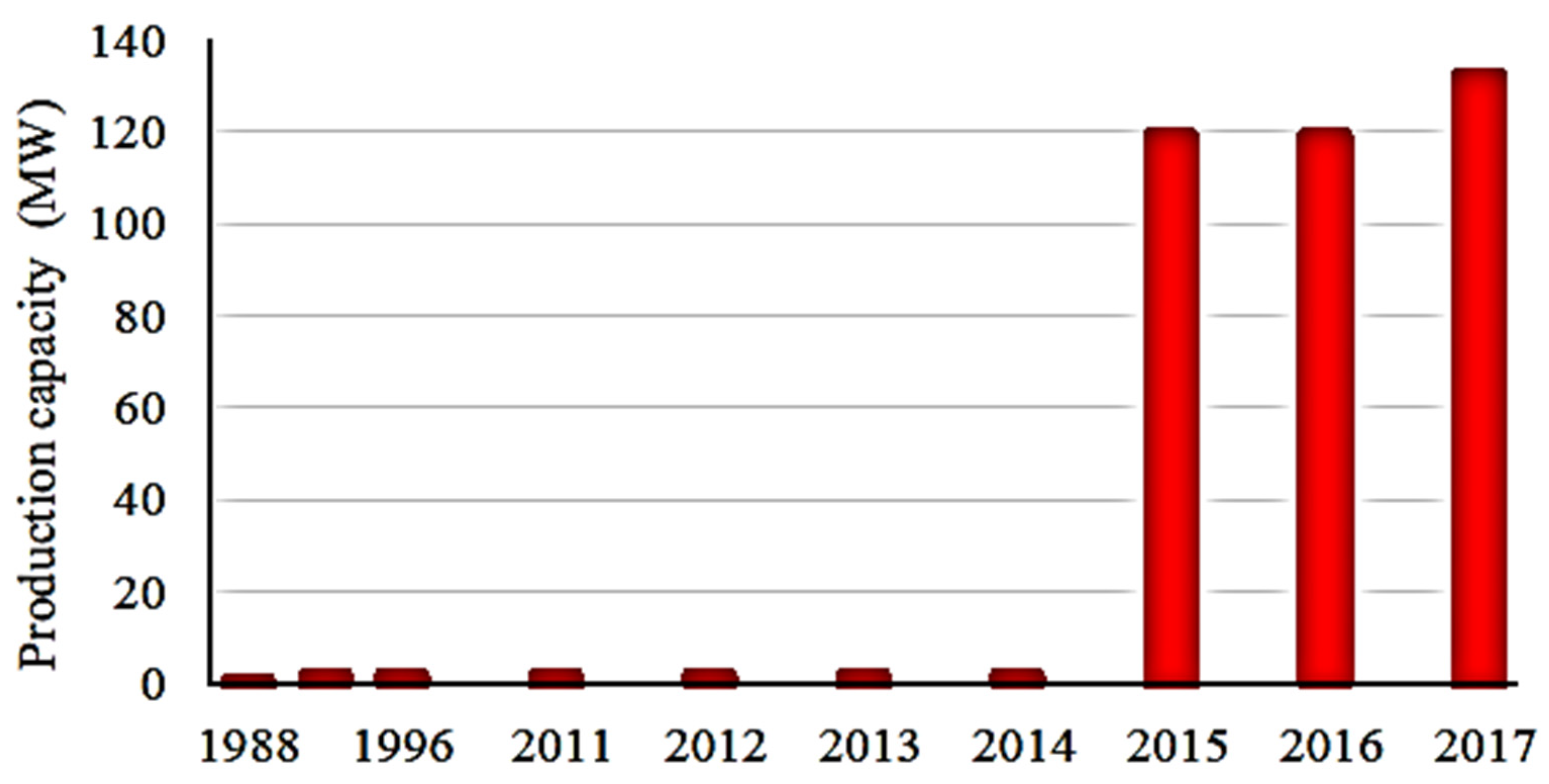
2. Evolution of Wind Energy in Jordan
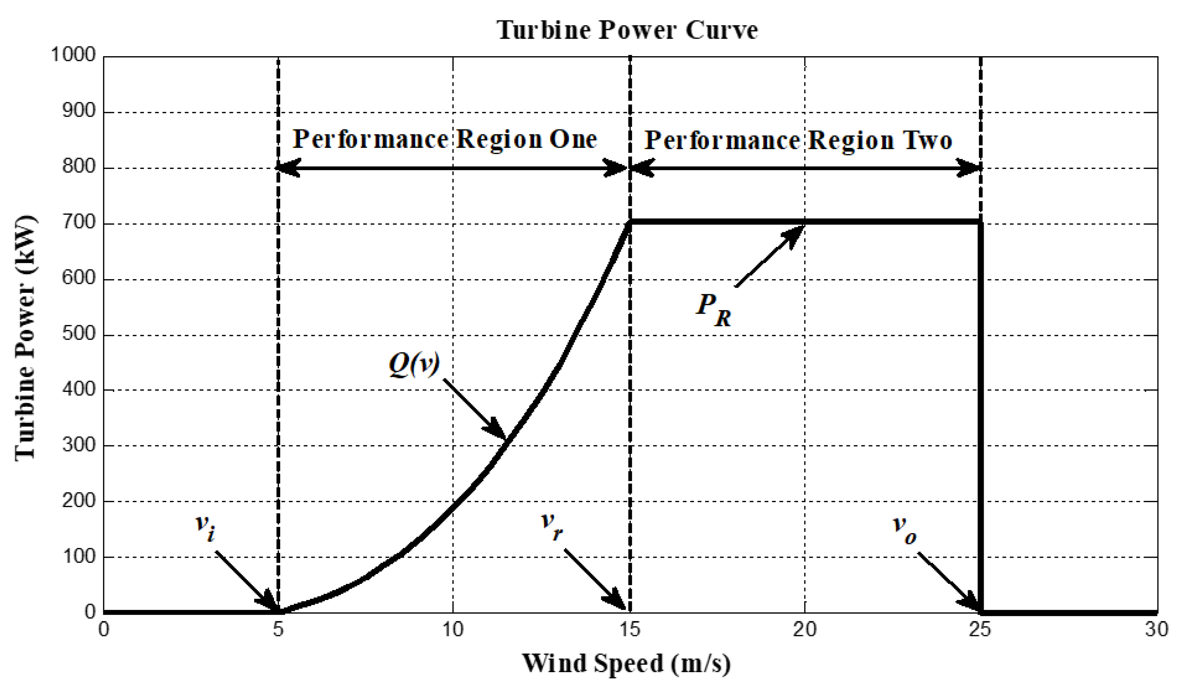
3. Energy Extracted from Different Wind Turbine Models
3.1. Energy Extracted by Q1(v) Based on Weibull Distribution
3.2. Energy Extracted by Q1(v) Based on Gamma Distribution
3.3. Energy Extracted by Q2(v) Based on Weibull and Gamma Distribution
3.4. Energy Extracted by Q3(v) Based on Weibull and Gamma Distribution
3.5. Energy Extracted by Q4(v) Based on Weibull and Gamma Distribution
3.6. Energy Extracted by Q5(v) Based on Weibull and Gamma Distribution
4. Cost Analysis
5. Capital Cost Model and Its Correction Factor
6. Optimization Problem
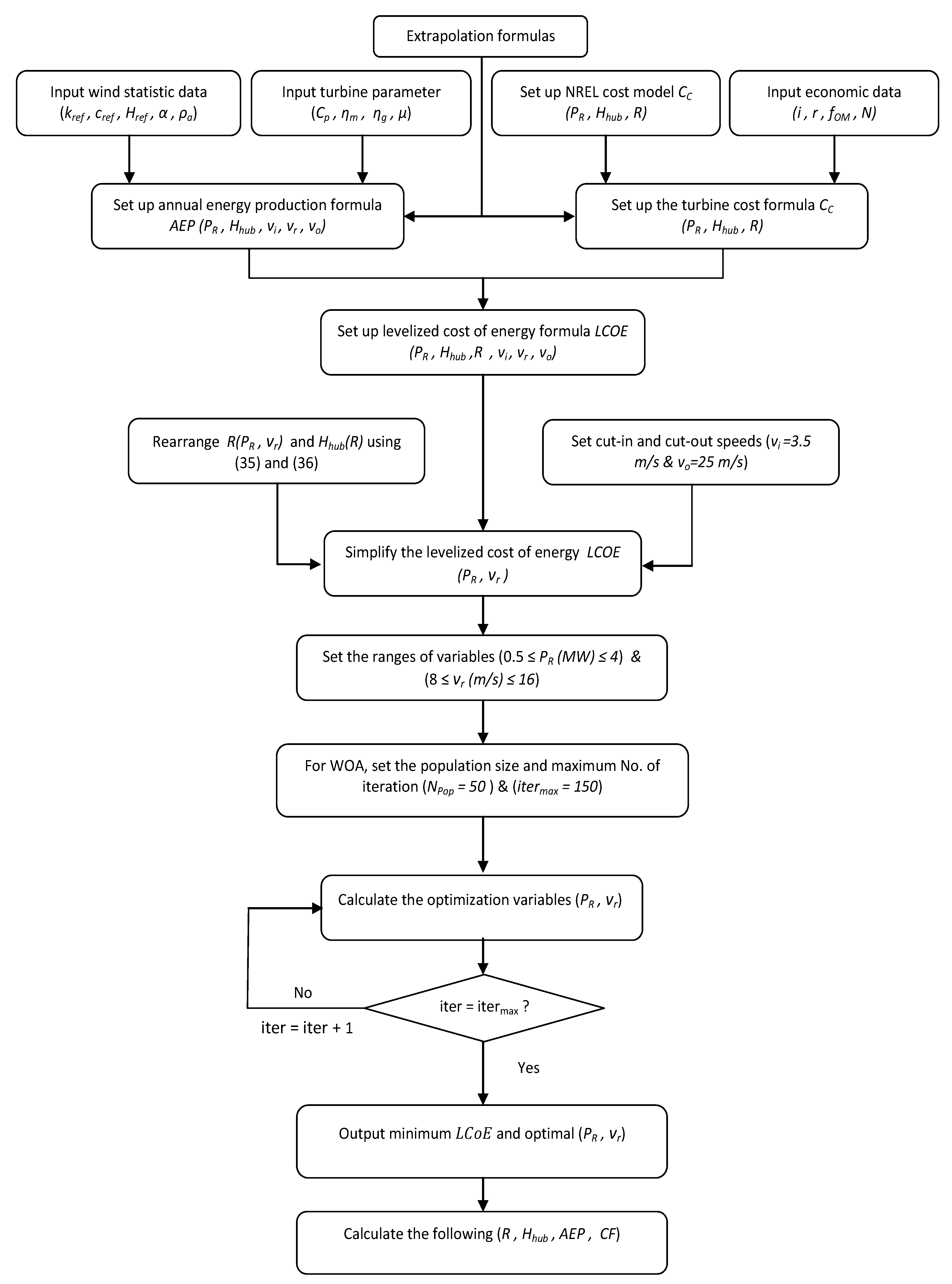
7. Extrapolation of Wind Speed at Different Height
8. Results and Discussion
9. Real Measurements and Validations Process
10. Conclusions
Author Contributions
Funding
Institutional Review Board Statement
Informed Consent Statement
Data Availability Statement
Acknowledgments
Conflicts of Interest
References
- De Castro, M.; Salvador, S.; Gómez-Gesteira, M.; Costoya, X.; Carvalho, D.; Sanz-Larruga, F.J.; Gimeno, L. Europe, China and the United States: Three different approaches to the development of offshore wind energy. Renew. Sustain. Energy Rev. 2019, 109, 55–70. [Google Scholar] [CrossRef]
- Calif, R.; Schmitt, F. Modeling of atmospheric wind speed sequence using a lognormal continuous stochastic equation. J. Wind Eng. Ind. Aerodyn. 2012, 109, 1–8. [Google Scholar] [CrossRef]
- Sathyajith, M. Wind Energy: Fundamentals, Resource Analysis and Economics; Springer: Berlin/Heidelberg, Germany, 2006. [Google Scholar]
- Ko, D.H.; Jeong, S.T.; Kim, Y.C. Assessment of wind energy for small-scale wind power in Chuuk State, Micronesia. Renew. Sustain. Energy Rev. 2015, 52, 613–622. [Google Scholar] [CrossRef]
- Han, Q.; Ma, S.; Wang, T.; Chu, F. Kernel density estimation model for wind speed probability distribution with applicability to wind energy assessment in China. Renew. Sustain. Energy Rev. 2019, 115, 109387. [Google Scholar] [CrossRef]
- Ladenburg, J.; Hevia-Koch, P.; Petrović, S.; Knapp, L. The offshore-onshore conundrum: Preferences for wind energy considering spatial data in Denmark. Renew. Sustain. Energy Rev. 2020, 121, 109711. [Google Scholar] [CrossRef]
- Peters, J.L.; Remmers, T.; Wheeler, A.J.; Murphy, J.; Cummins, V. A systematic review and meta-analysis of GIS use to reveal trends in offshore wind energy research and offer insights on best practices. Renew. Sustain. Energy Rev. 2020, 128, 109916. [Google Scholar] [CrossRef]
- Rosales-Asensio, E.; Borge-Diez, D.; Blanes-Peiró, J.-J.; Pérez-Hoyos, A.; Comenar-Santos, A. Review of wind energy technology and associated market and economic conditions in Spain. Renew. Sustain. Energy Rev. 2019, 101, 415–427. [Google Scholar] [CrossRef]
- Carrillo, C.; Obando Montaño, A.F.; Cidrás, J.; Díaz-Dorado, E. Review of power curve modelling for wind turbines. Renew. Sustain. Energy Rev. 2013, 21, 572–581. [Google Scholar] [CrossRef]
- Jiang, H.; Wang, J.; Wu, J.; Geng, W. Comparison of numerical methods and metaheuristic optimization algorithms for estimating parameters for wind energy potential assessment in low wind regions. Renew. Sustain. Energy Rev. 2017, 69, 1199–1217. [Google Scholar] [CrossRef]
- Wang, J.; Hu, J.; Ma, K. Wind speed probability distribution estimation and wind energy assessment. Renew. Sustain. Energy Rev. 2016, 60, 881–899. [Google Scholar] [CrossRef]
- Pishgar-Komleh, S.H.; Keyhani, A.; Sefeedpari, P. Wind speed and power density analysis based on Weibull and Rayleigh distributions (a case study: Firouzkooh county of Iran). Renew. Sustain. Energy Rev. 2015, 42, 313–322. [Google Scholar] [CrossRef]
- Wu, J.; Wang, J.; Chi, D. Wind energy potential assessment for the site of Inner Mongolia in China. Renew. Sustain. Energy Rev. 2013, 21, 215–228. [Google Scholar] [CrossRef]
- Jung, C.; Schindler, D. Wind speed distribution selection—A review of recent development and progress. Renew. Sustain. Energy Rev. 2019, 114, 109290. [Google Scholar] [CrossRef]
- Genç, M.S.; Çelik, M.; Karasu, İ. A review on wind energy and wind–hydrogen production in Turkey: A case study of hydrogen production via electrolysis system supplied by wind energy conversion system in Central Anatolian Turkey. Renew. Sustain. Energy Rev. 2012, 16, 6631–6646. [Google Scholar] [CrossRef]
- Yeom, J.-M.; Deo, R.C.; Adamwoski, J.F.; Chae, T.; Kim, D.-S.; Han, K.-S.; Kim, D.-Y. Exploring solar and wind energy resources in North Korea with COMS MI geostationary satellite data coupled with numerical weather prediction reanalysis variables. Renew. Sustain. Energy Rev. 2019, 119, 109570. [Google Scholar] [CrossRef]
- Elsner, P. Continental-scale assessment of the African offshore wind energy potential: Spatial analysis of an under-appreciated renewable energy resource. Renew. Sustain. Energy Rev. 2019, 104, 394–407. [Google Scholar] [CrossRef] [Green Version]
- Chen, X.; Foley, A.; Zhang, Z.; Wang, K.; O’Driscoll, K. An assessment of wind energy potential in the Beibu Gulf considering the energy demands of the Beibu Gulf Economic Rim. Renew. Sustain. Energy Rev. 2019, 119, 109605. [Google Scholar] [CrossRef]
- Kazimierczuk, A.H. Wind energy in Kenya: A status and policy framework review. Renew. Sustain. Energy Rev. 2019, 107, 434–445. [Google Scholar] [CrossRef]
- Li, Y.; Huang, X.; Tee, K.F.; Li, Q.; Wu, X.-P. Comparative study of onshore and offshore wind characteristics and wind energy potentials: A case study for southeast coastal region of China. Sustain. Energy Technol. Assess. 2020, 39, 100711. [Google Scholar] [CrossRef]
- Bilir, L.; İmir, M.; Devrim, Y.; Albostan, A. Seasonal and yearly wind speed distribution and wind power density analysis based on Weibull distribution function. Int. J. Hydrog. Energy 2015, 40, 15301–15310. [Google Scholar] [CrossRef]
- Chang, T.P. Estimation of wind energy potential using different probability density functions. Appl. Energy 2011, 88, 1848–1856. [Google Scholar] [CrossRef]
- Boudia, S.M.; Benmansour, A.; TabetHellal, M.A. Wind resource assessment in Algeria. Sustain. Cities Soc. 2016, 22, 171–183. [Google Scholar] [CrossRef]
- Azad, K.; Mohammad, R.; Halder, P.; Sutariya, J. Assessment of Wind Energy Prospect by Weibull Distribution for Prospective Wind Sites in Australia. Energy Procedia 2019, 160, 348–355. [Google Scholar] [CrossRef]
- Gugliani, G.K.; Sarkar, A.; Ley, C.; Mandal, S. New methods to assess wind resources in terms of wind speed, load, power and direction. Renew. Energy 2018, 129, 168–182. [Google Scholar] [CrossRef]
- Saeed, M.A.; Ahmed, Z.; Yang, J.; Zhang, W. An optimal approach of wind power assessment using Chebyshev metric for determining the Weibull distribution parameters. Sustain. Energy Technol. Assess. 2020, 37, 100612. [Google Scholar] [CrossRef]
- Alrashidi, M.; Rahman, S.; Pipattanasomporn, M. Metaheuristic optimization algorithms to estimate statistical distribution parameters for characterizing wind speeds. Renew. Energy 2020, 149, 664–681. [Google Scholar] [CrossRef]
- Dong, Y.; Wang, J.; Jiang, H.; Shi, X. Intelligent optimized wind resource assessment and wind turbines selection in Huitengxile of Inner Mongolia, China. Appl. Energy 2013, 109, 239–253. [Google Scholar] [CrossRef]
- Wang, J.; Huang, X.; Li, Q.; Ma, X. Comparison of seven methods for determining the optimal statistical distribution parameters: A case study of wind energy assessment in the large-scale wind farms of China. Energy 2018, 164, 432–448. [Google Scholar] [CrossRef]
- Aries, N.; Boudia, S.M.; Ounis, H. Deep assessment of wind speed distribution models: A case study of four sites in Algeria. Energy Convers. Manag. 2018, 155, 78–90. [Google Scholar] [CrossRef]
- Al-Quraan, A.; Stathopoulos, T.; Pillay, P. Comparison of Wind Tunnel and on Site Measurements for Urban Wind Energy Estimation of Potential Yields. J. Wind Eng. Ind. Aerodyn. 2016, 158, 1–10. [Google Scholar] [CrossRef] [Green Version]
- Stathopoulos, T.; Alrawashdeh, H.; Al-Quraan, A.; Blocken, B.; Dilimulati, A.; Paraschivoiu, M.; Pillay, P. Urban Wind Energy: Some Views on Potential and Challenges. J. Wind Eng. Ind. Aerodyn. 2018, 179, 146–157. [Google Scholar] [CrossRef]
- Al-Quraan, A.; Pillay, P.; Stathopoulos, T. Use of a Wind Tunnel for Urban Wind Power Estimation. In Proceedings of the IEEE Power & Energy Society General Meeting, Washington, DC, USA, 27–31 July 2014. [Google Scholar]
- Al-Quraan, A.; Stathopoulos, T.; Pillay, P. Estimation of Urban Wind Energy-Equiterre Building Case in Montreal. In Proceedings of the International Civil Engineering for Sustainability and Resilience Conference (CESARE’14), Irbid, Jordan, 24–27 April 2014. [Google Scholar]
- Alsaad, M. Wind energy potential in selected areas in Jordan. Energy Convers. Manag. 2013, 65, 704–708. [Google Scholar] [CrossRef]
- Bataineh, K.M.; Dalalah, D. Assessment of wind energy potential for selected areas in Jordan. Renew. Energy 2013, 59, 75–81. [Google Scholar] [CrossRef]
- Khraiwish Dalabeeh, A.S. Techno-economic analysis of wind power generation for selected locations in Jordan. Renew. Energy 2017, 101, 1369–1378. [Google Scholar] [CrossRef]
- Anani, A.; Zuamot, S.; Abu-Allan, F.; Jibril, Z. Evaluation of wind energy as a power generation source in a selected site in Jordan. Sol. Wind Technol. 1988, 5, 67–74. [Google Scholar] [CrossRef]
- Habali, S.M.; Hamdan, M.A.S.; Jubran, B.A.; Zaid, A.I.O. Wind speed and wind energy potential of Jordan. Sol. Energy 1987, 38, 59–70. [Google Scholar] [CrossRef]
- Amr, M.; Petersen, H.; Habali, S. Assessment of wind farm economics in relation to site wind resources applied to sites in Jordan. Sol. Energy 1990, 45, 167–175. [Google Scholar] [CrossRef]
- Ammari, H.D.; Al-Rwashdeh, S.S.; Al-Najideen, M.I. Evaluation of wind energy potential and electricity generation at five locations in Jordan. Sustain. Cities Soc. 2015, 15, 135–143. [Google Scholar] [CrossRef]
- Al-Quraan, A.; Alrawashdeh, H. Correlated Capacity Factor Strategy for Yield Maximization of Wind Turbine Energy. In Proceedings of the IEEE 5th International Conference on Renewable Energy Generation and Applications (ICREGA), Al-Ain, United Arab Emirates, 26–28 February 2018. [Google Scholar]
- Al-Quraan, A.; Al-Mahmodi, M.; Hussein, A.R.; Al-Masri, M.K. Comparative study between measured and estimated wind energy yield. Turk. J. Electr. Eng. Comp. Sci. 2020, 28, 2926–2939. [Google Scholar] [CrossRef]
- Al-Quraan, A.; Al-Qaisi, M. Modelling, Design and Control of a Standalone Hybrid PV-Wind Micro-Grid System. Energies 2021, 14, 4849. [Google Scholar] [CrossRef]
- Al-Mhairat, B.; Al-Quraan, A. Assessment of Wind Energy Resources in Jordan Using Different Optimization Techniques. Processes 2022, 10, 105. [Google Scholar] [CrossRef]
- Blanco, M.I. The economics of wind energy. Renew. Sustain Energy Rev. 2009, 13, 1372–1382. [Google Scholar] [CrossRef]
- Manwell, J.F.; McGowan, J.G.; Rogers, A.L. Wind Energy Explained: Theory, Design and Application, 2nd ed.; Wiley & Sons: Hoboken, NJ, USA, 2010. [Google Scholar]
- Nelson, V.; Starcher, K. Wind Energy: Renewable Energy and the Environment, 3rd ed.; CRC Press: Boca Raton, FL, USA, 2018. [Google Scholar]
- Perkin, S.; Garrett, D.; Jensson, P. Optimal wind turbine selection methodology: A case-study for Búrfell, Iceland. Renew. Energy 2015, 75, 165–172. [Google Scholar] [CrossRef]
- Rezaei Mirghaed, M.; Roshandel, R. Site specific optimization of wind turbines energy cost: Iterative approach. Energy Convers. Manag. 2013, 73, 167–175. [Google Scholar] [CrossRef]
- Fingersh, L.J.; Hand, M.M.; Laxson, A.S. Wind Turbine Design Cost and Scaling Model; National Renewable Energy Laboratory: Golden, CO, USA, 2006. [Google Scholar]
- Letcher, T.M. Wind Energy Engineering: A Handbook for Onshore and Offshore Wind Turbines, 1st ed.; Academic Press: Cambridge, MA, USA, 2017. [Google Scholar]
- Radaideh, A.; Bodoor, M.; Al-Quraan, A. Active and Reactive Power Control for Wind Turbines Based DFIG Using LQR Controller with Optimal Gain-Scheduling. J. Electr. Comp. Eng. 2021, 2021, 1218236. [Google Scholar] [CrossRef]
- Al-Quraan, A.; Al-Mahmodi, M.; Al-Asemi, T.; Bafleh, A.; Bdour, M.; Muhsen, H.; Malkawi, A. A New Configuration of Roof Photovoltaic System for Limited Area Applications—A Case Study in KSA. Buildings 2022, 12, 92. [Google Scholar] [CrossRef]
- Walker, R.P.; Swift, A. Wind Energy Essentials: Societal, Economic, and Environmental Impacts, 1st ed.; Wiley & Sons: Hoboken, NJ, USA, 2015. [Google Scholar]
- Eminoglu, U.; Turksoy, O. Power curve modeling for wind turbine systems: A comparison study. Int. J. Ambient Energy 2019, 42, 1912–1921. [Google Scholar] [CrossRef]
- Stehly, T.; Beiter, P.; Duffy, P. 2019 Cost of Wind Energy Review; National Renewable Energy Laboratory: Golden, CO, USA, 2020. Available online: https://www.nrel.gov/docs/fy21osti/78471.pdf (accessed on 23 January 2022).
- Forbes, C.; Evans, M.; Hastings, N.; Peacock, B. Statistical Distributions, 4th ed.; Wiley & Sons: Hoboken, NJ, USA, 2010. [Google Scholar]
- Bortolotti, P.; Berry, D.; Murray, R.; Gaertner, E.; Jenne, D.; Damiani, R.; Barter, G.; Dykes, K. A Detailed Wind Turbine Blade Cost Model; Technical Report NREL/TP-5000-73585; National Renewable Energy Laboratory: Golden, CO, USA, 2019. Available online: https://www.nrel.gov/docs/fy19osti/73585.pdf (accessed on 23 January 2022).
- Shahab, S.; Lades, L. Sludge and transaction costs. Behav. Public Policy. 2021, pp. 1–22. Available online: https://www.cambridge.org/core/journals/behavioural-public-policy/article/sludge-and-transaction-costs/D09206BF9B36C129F40A27A9E749074B (accessed on 23 January 2022).
- Cavusoglu, S.S.; Macário, R. Minimum delay or maximum efficiency? Rising productivity of available capacity at airports: Review of current practice and future needs. J. Air Transp. Manag. 2021, 90, 101947. [Google Scholar] [CrossRef]
- Foryś, I.; Głuszak, M.; Konowalczuk, J. Compensation due to land use restrictions: The case of limited use area in the vicinity of Polish airports. Oecon. Copernic. 2019, 10, 649–667. [Google Scholar] [CrossRef] [Green Version]
- Masdar Co. Tafilah Wind Farm. 2021. Available online: https://masdar.ae/en/masdar-clean-energy/projects/tafila-wind-farm (accessed on 23 January 2022).
- Elecnor Group. Al-Rajef Wind Farm. 2021. Available online: https://www.elecnor.com/resources/files/1/projects/en/referencia-al-rajef-wind-farm-jordan-en.pdf (accessed on 23 January 2022).
- Alcazar Energy. Al-Rajef Wind Farm. 2021. Available online: https://alcazarenergy.com/wp-content/uploads/2021/01/Project-Fact-Sheets_Al-Rajef-86MW.pdf (accessed on 23 January 2022).
- KOSPO Co-Funds $101 m 51.75 MW Wind Farm in Jordan. (2 October 2018). 2021. Available online: https://asian-power.com/project/news/kospo-co-funds-101m-5175mw-wind-farm-in-jordan (accessed on 23 January 2022).
- IFC Funds New Wind Power Plant in Jordan. (7 November 2018). 2021. Available online: https://www.petra.gov.jo/Include/InnerPage.jsp?ID=11309&lang=en&name=en_news (accessed on 23 January 2022).
- Ministry of Energy and Mineral Resources—Jordan. Daihan Wind Project. 2021. Available online: https://www.memr.gov.jo/Ar/NewsDetails/%D8%B2%D9%88%D8%A7%D8%AA%D9%8A_%D8%AA%D8%AF%D8%B4%D9%86_%D9%85%D8%B4%D8%B1%D9%88%D8%B9_%D8%AF%D8%A7%D9%8A%D9%87%D8%A7%D9%86_%D9%84%D8%B7%D8%A7%D9%82%D8%A9_%D8%A7%D9%84%D8%B1%D9%8A%D8%A7%D8%AD_%D9%81%D9%8A_%D8%A7%D9%84%D8%B7%D9%81%D9%8A%D9%84%D8%A9 (accessed on 23 January 2022).
- Alcazar Energy. Shobak Wind Farm. 2021. Available online: https://alcazarenergy.com/wp-content/uploads/2021/01/Project-Fact-Sheets_Shobak-Wind.pdf (accessed on 23 January 2022).
- Jordan’s Fujeij Wind Energy Project Inaugurated. (16 October 2019). 2021. Available online: https://www.evwind.es/2019/10/16/jordans-fujeij-wind-energy-project-inaugurated/71345 (accessed on 23 January 2022).
- Korea’s KEPCO Opens 89-MW Wind Park in Jordan. (17 October 2019). 2021. Available online: https://renewablesnow.com/news/koreas-kepco-opens-89-mw-wind-park-in-jordan-672962/ (accessed on 23 January 2022).
- Elecnor Co. Ma’an Wind Farm. 2021. Available online: https://www.elecnor.com/resources/files/1/projects/en/referencia-maan-jordan-en.pdf (accessed on 23 January 2022).
- Wind Energy in Jordan, Awards Siemens Gamesa Contract for 80 MW Wind Farm. (24 July 2019). 2021. Available online: https://www.evwind.es/2019/11/24/wind-energy-in-jordan-awards-siemens-gamesa-contract-for-80-mw-wind-farm/71984 (accessed on 23 January 2022).
- Ministry of Energy and Mineral Resources—Jordan. Ma’an Wind Farm. 2021. Available online: https://www.memr.gov.jo/Ar/NewsDetails/%D8%A7%D9%81%D8%AA%D8%AA%D8%A7%D8%AD_%D9%85%D8%B4%D8%B1%D9%88%D8%B9_%D8%B7%D8%A7%D9%82%D8%A9_%D8%A7%D9%84%D8%B1%D9%8A%D8%A7%D8%AD_%D9%81%D9%8A_%D9%85%D8%B9%D8%A7%D9%86 (accessed on 23 January 2022).
- Wind Farms in Jordan. 2021. Available online: https://www.thewindpower.net/windfarms_list_en.php?country=JO (accessed on 23 January 2022).
- Hu, J.; Harmsen, R.; Crijns-Graus, W.; Worrell, E. Geographical optimization of variable renewable energy capacity in China using modern portfolio theory. Appl. Energy 2019, 253, 113614. [Google Scholar] [CrossRef]
- Gualtieri, G.; Secci, S. Methods to extrapolate wind resource to the turbine hub height based on power law: A 1-h wind speed vs. Weibull distribution extrapolation comparison. Renew. Energy 2012, 43, 183–200. [Google Scholar] [CrossRef]
- Chen, J.; Wang, F.; Stelson, K.A. A mathematical approach to minimizing the cost of energy for large utility wind turbines. Appl. Energy 2018, 228, 1413–1422. [Google Scholar] [CrossRef]
- Central Bank of Jordan, (15 December 2020). Central Bank Interest Rates. 2021. Available online: https://www.cbj.gov.jo/Pages/viewpage.aspx?pageID=259 (accessed on 23 January 2022).
- Central Bank of Jordan, (4 February 2021). Economic Indicators. 2021. Available online: https://www.cbj.gov.jo/Pages/viewpage.aspx?pageID=282 (accessed on 23 January 2022).

| Project | Number of Turbines | Turbine Model | Turbine Rated Power (kW) | VI (m/s) | VR (m/s) | Vo (m/s) | Hub Height (m) | Total Capacity (MW) |
|---|---|---|---|---|---|---|---|---|
| Tafila | 38 | Vestas V112/3075 | 3075 | 2.5 | 13 | 25 | 84 | 116.85 |
| Hofa | 5 | Vestas V27/225 | 2250 | 3.5 | 14 | 22 | 33.5 | 1.125 |
| Fujeij | 27 | Gamesa G126/3300 | 3300 | 2.5 | 12 | 25 | 117 | 89.1 |
| Al Rajef | 41 | Gamesa G114/2000 | 2000 | 3 | 11 | 25 | 80 | 86.1 |
| Daehan | 15 | Vestas V136/3450 | 3450 | 2.5 | 11 | 22 | 149 | 51.75 |
| Project Name | Turbine Model | Number of Turbines | Overall Real Cost (Million $) | Real Cost per Turbine (Million $) | Model Cost per Turbine (Million $) | Scaling Factor | |
|---|---|---|---|---|---|---|---|
| Jordan Wind—Tafileh [63,75] | Vestas(V112/3.075) 84m HH | 4 | 287 | (10.53%) 30.2211 | 7.555275 | 3.687782 | 2.0487 |
| Vestas(V112/3.075) 94m HH | 34 | (89.47%) 256.7789 | 7.552321 | 3.762716 | 2.0071 | ||
| AlRajef [64,65,75] | Gamesa(114/2.100) 80m HH | 41 | 184.6 | 4.502439 | 3.087002 | 1.4585 | |
| Deahan [66,67,68,75] | Vestas(V136/3.450) 112m HH | 15 | 102 | 6.800000 | 5.411168 | 1.2567 | |
| Shobak [69,75] | Vestas(V136/3.450) 112m HH | 13 | 104 | 8.000000 | 5.411168 | 1.4784 | |
| Fujejji [70,71,75] | Vestas(V126/3.300) 117m HH | 27 | 180 | 6.666667 | 4.785160 | 1.3932 | |
| Al-Hussein University [72,73,74,75] | Gamesa(97/2.000) 78m HH | 40 | 148 | 3.700000 | 2.407814 | 1.5367 | |
| Average Scaling Factor | 1.5970 ≈ 1.6 | ||||||
| Wind Site | Longitude and Latitude | Average Wind Speed (m/s) |
|---|---|---|
| Queen Alia Airport | 35°59′21.59″ E, 31°43′12.59″ N | 7.25 |
| Amman Civil Airport | 35°59′17.39″ E, 31°58′12.59″ N | 6.7 |
| King Hussein Airport | 35°01′3.02″ E, 29°36′25.09″ N | 5.93 |
| Irbid | 35°51′25.751″ E, 32°32′43.591″ N | 6.58 |
| Mafraq | 36°11′60.00″ E, 32°20′59.99″ N | 7.63 |
| Ma’an | 35°44′3.2676″ E, 30°11′41.8488″N | 8.11 |
| Safawi | 37°126′2763″ E, 32°19′2941″ N | 7.1 |
| Irwaished | 38°7′26″ E, 32°18′5″ N | 6.1 |
| Ghor Es Safi | 35°27′55.58″ E, 31°02′9.89″ N | 5.8 |
| Wind Site | Shape Factor | Shear Exponent A | ||
|---|---|---|---|---|
| Queen Alia Airport | 4.02 | 1.17 | 10 | 0.15 |
| Amman Civil Airport | 3.48 | 1.15 | 10 | 0.15 |
| King Hussein Airport | 2.78 | 5.93 | 10 | 0.21 |
| Irbid | 7.33 | 0.30 | 10 | 0.25 |
| Mafraq | 5.33 | 0.71 | 10 | 0.15 |
| Ma’an | 8.62 | 0.46 | 10 | 0.15 |
| Safawi | 6.50 | 0.76 | 10 | 0.15 |
| Irwaished | 4.52 | 0.91 | 10 | 0.15 |
| Ghor Es Safi | 6.71 | 0.36 | 10 | 0.20 |
| Parameter | Value |
|---|---|
| No. of blades | 3 |
| Air density | 1.225 Kg/m3 |
| 0.45 [9,78] | |
| 0.96 [78] | |
| 0.97 [78] | |
| 0.15 [51] | |
| Cut–in speed (vi) | 3.5 m/s |
| Cut–out speed (vo) | 25 m/s |
| 2.5% [79] | |
| 0.3% [80] | |
| 3.5% [3] | |
| 20 year [3,51] |
| Site | Queen Alia Airport | Amman Civil Airport | ||||||||
|---|---|---|---|---|---|---|---|---|---|---|
| Model | Q1(v) | Q2(v) | Q3(v) | Q4(v) | Q5(v) | Q1(v) | Q2(v) | Q3(v) | Q4(v) | Q5(v) |
| k | 4.02 | 4.02 | 4.02 | 4.02 | 4.02 | 3.48 | 3.48 | 3.48 | 3.48 | 3.48 |
| c (m/s) | 1.6 | 1.6 | 1.59 | 1.59 | 1.6 | 1.58 | 1.57 | 1.57 | 1.57 | 1.58 |
| Vr (m/s) | 10.59 | 9.63 | 10.25 | 9.7 | 9.72 | 10.21 | 9.12 | 9.69 | 9.22 | 9.26 |
| Pr (MW) | 1.48 | 1.13 | 1.25 | 1.12 | 1.21 | 1.46 | 1 | 1.12 | 1 | 1.11 |
| R (m) | 39.33 | 39.54 | 37.96 | 39.02 | 40.32 | 41.21 | 40.47 | 39.04 | 39.84 | 41.64 |
| H (m) | 79.22 | 79.55 | 77.1 | 78.76 | 80.75 | 82.12 | 80.99 | 78.78 | 80.02 | 82.76 |
| Site | King Hussein Airport | Irbid | ||||||||
| Model | Q1(v) | Q2(v) | Q3(v) | Q4(v) | Q5(v) | Q1(v) | Q2(v) | Q3(v) | Q4(v) | Q5(v) |
| k | 3.42 | 3.43 | 3.4 | 3.43 | 3.43 | 7.33 | 7.33 | 7.33 | 7.33 | 7.33 |
| c (m/s) | 9.33 | 9.39 | 9.24 | 9.38 | 9.42 | 0.58 | 0.58 | 0.57 | 0.57 | 0.59 |
| Vr (m/s) | 10.77 | 10.22 | 11.1 | 10.21 | 10.18 | 8 | 8 | 8 | 8 | 8 |
| Pr (MW) | 1.8 | 1.67 | 1.75 | 1.64 | 1.7 | 2.72 | 2.85 | 2.15 | 2.4 | 3.07 |
| R (m) | 42.26 | 44.01 | 39.85 | 43.75 | 44.66 | 81.16 | 83.04 | 72.16 | 76.17 | 86.2 |
| H (m) | 83.72 | 86.35 | 80.03 | 85.96 | 87.34 | 138.03 | 140.48 | 126.14 | 131.48 | 144.56 |
| Site | Mafraq | Ma’an | ||||||||
| Model | Q1(v) | Q2(v) | Q3(v) | Q4(v) | Q5(v) | Q1(v) | Q2(v) | Q3(v) | Q4(v) | Q5(v) |
| k | 5.33 | 5.33 | 5.33 | 5.33 | 5.33 | 8.62 | 8.62 | 8.62 | 8.62 | 8.62 |
| c (m/s) | 0.98 | 0.97 | 0.97 | 0.97 | 0.98 | 0.63 | 0.63 | 0.62 | 0.62 | 0.63 |
| Vr (m/s) | 9.42 | 8.19 | 8.84 | 8.31 | 8.3 | 8.92 | 8 | 8.48 | 8 | 8 |
| Pr (MW) | 1.34 | 0.75 | 0.88 | 0.75 | 0.85 | 1.2 | 0.75 | 0.77 | 0.68 | 0.82 |
| R (m) | 44.56 | 41.13 | 39.85 | 40.22 | 43.05 | 45.8 | 42.72 | 39.65 | 40.69 | 44.64 |
| H (m) | 87.19 | 81.99 | 80.02 | 80.59 | 84.91 | 89.03 | 84.41 | 79.73 | 81.31 | 87.3 |
| Site | Safawi | Irwaished | ||||||||
| Model | Q1(v) | Q2(v) | Q3(v) | Q4(v) | Q5(v) | Q1(v) | Q2(v) | Q3(v) | Q4(v) | Q5(v) |
| k | 6.5 | 6.5 | 6.5 | 6.5 | 6.5 | 4.52 | 4.52 | 4.52 | 4.52 | 4.52 |
| c (m/s) | 1.04 | 1.04 | 1.03 | 1.04 | 1.04 | 1.25 | 1.24 | 1.24 | 1.24 | 1.24 |
| Vr (m/s) | 10.18 | 9.23 | 9.98 | 9.29 | 9.28 | 9.92 | 8.81 | 9.44 | 8.91 | 8.92 |
| Pr (MW) | 1.4 | 1.01 | 1.18 | 1 | 1.08 | 1.4 | 0.91 | 1.05 | 0.91 | 1.01 |
| R (m) | 40.52 | 39.85 | 38.4 | 39.26 | 40.91 | 42.23 | 40.65 | 39.33 | 39.94 | 42.08 |
| H (m) | 81.06 | 80.03 | 77.78 | 79.12 | 81.66 | 83.67 | 81.26 | 79.23 | 80.17 | 83.44 |
| Site | Ghor Es Safi | |||||||||
| Model | Q1(v) | Q2(v) | Q3(v) | Q4(v) | Q5(v) | |||||
| k | 6.7 | 6.7 | 6.7 | 6.7 | 6.7 | |||||
| c (m/s) | 0.59 | 0.59 | 0.58 | 0.59 | 0.6 | |||||
| Vr (m/s) | 8.04 | 8 | 8 | 8 | 8 | |||||
| Pr (MW) | 2.1 | 2.17 | 1.62 | 1.77 | 2.35 | |||||
| R (m) | 70.68 | 72.54 | 62.6 | 65.5 | 75.51 | |||||
| H (m) | 124.15 | 126.65 | 113.13 | 117.12 | 130.61 | |||||
| Site | Queen Alia Airport | Amman Civil Airport | ||||||||
|---|---|---|---|---|---|---|---|---|---|---|
| Model | Q1(v) | Q2(v) | Q3(v) | Q4(v) | Q5(v) | Q1(v) | Q2(v) | Q3(v) | Q4(v) | Q5(v) |
| AEP (MWh) | 3721.85 | 3000.81 | 3949.3 | 3011.24 | 3041.65 | 2852.56 | 2157.12 | 2918.06 | 2184.02 | 2215.87 |
| CF | 0.29 | 0.3 | 0.36 | 0.31 | 0.29 | 0.22 | 0.25 | 0.3 | 0.25 | 0.23 |
| LCoE ($/MWh) | 67.9 | 75.2 | 56.56 | 73.45 | 78.39 | 93.47 | 103.65 | 75.75 | 100.01 | 109.24 |
| Site | King Hussein Airport | Irbid | ||||||||
| Model | Q1(v) | Q2(v) | Q3(v) | Q4(v) | Q5(v) | Q1(v) | Q2(v) | Q3(v) | Q4(v) | Q5(v) |
| AEP (MWh) | 7573.1 | 7169.74 | 8275.35 | 7061.56 | 7168.75 | 3755.52 | 3719.72 | 4341.78 | 3320.47 | 3611.04 |
| CF | 0.48 | 0.49 | 0.54 | 0.49 | 0.48 | 0.16 | 0.15 | 0.23 | 0.16 | 0.13 |
| LCoE ($/MWh) | 40.2 | 43.21 | 33.81 | 43.22 | 44.47 | 287.6 | 308.61 | 183.22 | 275.48 | 351.42 |
| Site | Mafraq | Ma’an | ||||||||
| Model | Q1(v) | Q2(v) | Q3(v) | Q4(v) | Q5(v) | Q1(v) | Q2(v) | Q3(v) | Q4(v) | Q5(v) |
| AEP (MWh) | 2571.06 | 1716.58 | 2472.59 | 1729.12 | 1784.36 | 2718.95 | 1969.03 | 2583.55 | 1837.73 | 1993.79 |
| CF | 0.22 | 0.26 | 0.32 | 0.26 | 0.24 | 0.26 | 0.3 | 0.38 | 0.31 | 0.28 |
| LCoE ($/MWh) | 111.92 | 121.7 | 84.48 | 116.32 | 131.45 | 106.37 | 113.5 | 76.84 | 108.79 | 124.1 |
| Site | Safawi | Irwaished | ||||||||
| Model | Q1(v) | Q2(v) | Q3(v) | Q4(v) | Q5(v) | Q1(v) | Q2(v) | Q3(v) | Q4(v) | Q5(v) |
| AEP (MWh) | 4110.25 | 3207.76 | 4387.37 | 3181.22 | 3261.82 | 2969.41 | 2164.48 | 3007.72 | 2179.65 | 2233.72 |
| CF | 0.34 | 0.36 | 0.42 | 0.36 | 0.35 | 0.24 | 0.27 | 0.33 | 0.27 | 0.25 |
| LCoE ($/MWh) | 62.17 | 68.16 | 50.38 | 66.98 | 71.52 | 91.34 | 100.61 | 72.41 | 97.11 | 106.77 |
| Site | Ghor Es Safi | |||||||||
| Model | Q1(v) | Q2(v) | Q3(v) | Q4(v) | Q5(v) | |||||
| AEP (MWh) | 2317.23 | 2286.6 | 2728.66 | 2021.04 | 2208.2 | |||||
| CF | 0.13 | 0.12 | 0.19 | 0.13 | 0.11 | |||||
| LCoE ($/MWh) | 327.02 | 352.68 | 203.93 | 308.11 | 405 | |||||
| Model Type | Fuhrlander-100 | |||||
|---|---|---|---|---|---|---|
| Study | Our Proposed Model | Study in Ref. [41] | ||||
| Site | Q. A. Airport | K. H. Airport | Safawi | Q. A. Airport | K. H. Airport | Safawi |
| AEP (MWh) | 147.97 | 235.11 | 148.79 | 60.42 | 313.45 | 147.42 |
| CF (%) | 16.9 | 26.8 | 17 | 6.8 | 35.7 | 16.8 |
| Model Type | EWT-500 | |||||
| Study | Our Proposed Model | Study in Ref. [41] | ||||
| Site | Q. A. Airport | K. H. Airport | Safawi | Q. A. Airport | K. H. Airport | Safawi |
| AEP (MWh) | 1390.16 | 2178.04 | 1530.07 | 556.6 | 2086.32 | 1257.11 |
| CF (%) | 31.7 | 49.7 | 34.9 | 12.7 | 47.6 | 28.7 |
| Model Type | EWT-900 | |||||
| Study | Our Proposed Model | Study in Ref. [41] | ||||
| Site | Q. A. Airport | K. H. Airport | Safawi | Q. A. Airport | K. H. Airport | Safawi |
| AEP (MWh) | 1403.23 | 2283.77 | 1422.53 | 582.94 | 2448.36 | 1379.99 |
| CF (%) | 17.8 | 29 | 18 | 7.3 | 31.1 | 17.5 |
| Model Type | Fuhrlander-1500 | |||||
| Study | Our Proposed Model | Study in Ref. [41] | ||||
| Site | Q. A. Airport | K. H. Airport | Safawi | Q. A. Airport | K. H. Airport | Safawi |
| AEP (MWh) | 3353.68 | 5786.03 | 3588.15 | 1342.87 | 5316.35 | 3091.99 |
| CF (%) | 25.5 | 44 | 27.3 | 10.2 | 40.4 | 23.5 |
| Model Type | Vestas-3000 | |||||
| Study | Our Proposed Model | Study in Ref. [41] | ||||
| Site | Q. A. Airport | K. H. Airport | Safawi | Q. A. Airport | K. H. Airport | Safawi |
| AEP (MWh) | 7445.04 | 13132.92 | 8056.58 | 2014.31 | 7974.53 | 4657.99 |
| CF (%) | 27.6 | 48.8 | 29.9 | 9.8 | 37.4 | 19.6 |
| Year | 2019 | |||
|---|---|---|---|---|
| Month | Tafila (MWh) | Hussein (MWh) | Al-Rajaf (MWh) | Al-Fajeej (MWh) |
| Jan | 44,405 | 14,720 | 30,830 | 3645 |
| Feb | 33,818 | 11,785 | 26,105 | 0 |
| Mar | 38,770 | 14,045 | 24,961 | 0 |
| Apr | 31,352 | 12,544 | 27,645 | 0 |
| May | 26,251 | 9334 | 19,461 | 0 |
| Jun | 30,315 | 7214 | 22,840 | 0 |
| Jul | 31,433 | 5748 | 23,151 | 17,908 |
| Aug | 28,968 | 4260 | 21,693 | 26,363 |
| Sep | 17,583 | 2357 | 12,660 | 18,566 |
| Oct | 16,526 | 3748 | 13,862 | 10,656 |
| Nov | 25,437 | 3646 | 20,160 | 20,400 |
| Dec | 37,692 | 9944 | 30,968 | 22,473 |
| Total | 362,550 | 99,345 | 274,336 | 120,011 |
| CF | 35.4% | 14.2% | 36.4% | 15.4% |
| Cost (JD/MWh) | 85 | 80 | 80 | 83 |
| Wind Farm Specifications | ||||
| Wind Farm Name | Turbine Model | Hub Height (m) | Capacity (MW) | No. of Turbines |
| Tafila | Vestas (V112/3.075) | 94/84 | 117 | 38 |
| Al–Hussein Uni. | Gamesa (G97/2.0) | 78 | 80 | 40 |
| Al-Rajaf | Gamesa (G114/2.1) | 80 | 86.1 | 41 |
| Al-Fajeej | Vestas (V126/3.3) | 117 | 89.1 | 27 |
| Month | Tafila | Al-Hussein Uni. | Al-Rajaf | Al-Fajeej | |||||
|---|---|---|---|---|---|---|---|---|---|
| vref (45m) | vhub (94m) | vhub (84m) | vref (51m) | vhub (78m) | vref (50m) | vhub (80m) | vref (50m) | vhub (117m) | |
| Jan | 10.69 | 11.51 | 11.38 | 6.64 | 6.93 | 6.58 | 6.9 | 7.08 | 7.71 |
| Feb | 9.23 | 9.94 | 9.82 | 7.48 | 7.8 | 6.94 | 7.27 | 8.05 | 8.76 |
| Mar | 9.69 | 10.43 | 10.31 | 7.22 | 7.53 | 6.44 | 6.75 | 6.67 | 7.26 |
| Apr | 9.08 | 9.77 | 9.66 | 5.5 | 5.74 | 6.25 | 6.55 | 6.78 | 7.38 |
| May | 7.82 | 8.42 | 8.32 | 6.29 | 6.56 | 6.85 | 7.18 | 6.41 | 6.98 |
| Jun | 8.16 | 8.78 | 8.69 | 6.87 | 7.17 | 6.74 | 7.06 | 7.1 | 7.73 |
| Jul | 7.79 | 8.39 | 8.29 | 6.84 | 7.14 | 5.91 | 6.19 | 5.88 | 6.4 |
| Aug | 7.6 | 8.18 | 8.09 | 5.93 | 6.19 | 6.53 | 6.84 | 6.47 | 7.04 |
| Sep | 6.28 | 6.76 | 6.68 | 5.81 | 6.06 | 6.2 | 6.5 | 5.2 | 5.66 |
| Oct | 5.86 | 6.31 | 6.24 | 4.56 | 4.76 | 5.78 | 6.06 | 5.09 | 5.54 |
| Nov | 8.86 | 9.54 | 9.43 | 4.02 | 4.19 | 6.23 | 6.53 | 5.52 | 6.01 |
| Dec | 9.38 | 10.1 | 9.98 | 5.24 | 5.47 | 7.07 | 7.41 | 6.71 | 7.31 |
| Parameter | Tafila | Al-Hussein Uni. | Al-Rajaf | Al-Fajeej |
|---|---|---|---|---|
| Cut—in speed (vi) | 2.5 | 3 | 1 | 3 |
| Rated speed(vr) | 13 | 14 | 11.5 | 12 |
| Cut—out speed (vo) | 25 | 25 | 25 | 22.5 |
| Wind Shear Exponent | 0.1 | 0.1 | 0.1 | 0.1 |
| Cost Scaling Factor | 2.03 | 1.54 | 1.46 | 1.39 |
| Economic Input Parameters | ||||
| Discount rate (r) for 2019 | 4% [79] | |||
| Inflation rate (i) for 2019 | 0.3% [80] | |||
| 3.5% | ||||
| Lifetime of system (N) | 20 years | |||
| Site | Tafila | Al-Hussein Uni. | ||||||
|---|---|---|---|---|---|---|---|---|
| Month | Emes | Eest | CFest | Error(%) | Emes | Eest | CFest | Error(%) |
| Jan | 44,405 | 46,589.81 | 53.59 | 4.92 | 14,720 | 14,646.19 | 24.61 | 0.5 |
| Feb | 33,818 | 37,664.58 | 47.97 | 11.37 | 11,785 | 16,722.98 | 31.11 | 41.9 |
| Mar | 38,770 | 43,522.91 | 50.06 | 12.26 | 14,045 | 17,345.31 | 29.14 | 23.5 |
| Apr | 31,352 | 39,685.5 | 47.17 | 26.58 | 12,544 | 8866.606 | 15.39 | 29.32 |
| May | 26,251 | 34,339.02 | 39.5 | 30.81 | 9334 | 12,937.44 | 21.74 | 38.61 |
| Jun | 30,315 | 35,147.79 | 41.78 | 15.94 | 7214 | 15,231.99 | 26.44 | 111.14 |
| Jul | 31,433 | 34,168.33 | 39.3 | 8.7 | 5748 | 15,603.9 | 26.22 | 171.47 |
| Aug | 28,968 | 32,954.05 | 37.91 | 13.76 | 4260 | 11,220.85 | 18.85 | 163.4 |
| Sep | 17,583 | 22,899.66 | 27.22 | 30.24 | 2357 | 10,278.15 | 17.84 | 336.07 |
| Oct | 16,526 | 20,440.06 | 23.51 | 23.68 | 3748 | 5073.311 | 8.52 | 35.36 |
| Nov | 25,437 | 38,723.56 | 46.03 | 52.23 | 3646 | 3058.701 | 5.31 | 16.11 |
| Dec | 37,692 | 42,325.31 | 48.69 | 12.29 | 9944 | 7964.85 | 13.38 | 19.9 |
| Total Eest | 428,460.6 | 138,950.28 | ||||||
| Total Emes | 362,550 | 111,345 | ||||||
| Error(%) | 18.18 | 19.6 | ||||||
| Overall CFest | 41.86 | 19.83 | ||||||
| Overall CFmes | 35.4 | 14.2 | ||||||
| LCOEest | 71.92 | 112.56 | ||||||
| LCOEmes | 119.89 | 112.84 | ||||||
| Site | Al-Rajaf | Al-Fajeej | ||||||
| Month | Emes | Eest | CFest | Error(%) | Emes | Eest | CFest | Error(%) |
| Jan | 30,830 | 22,634.64 | 35.33 | 26.58 | 3645 | 5907.97 | 39.08 | 36.8 |
| Feb | 26,105 | 22,151.01 | 38.28 | 15.15 | 18,166 | 14,151.1 | 22.06 | 23.78 |
| Mar | 24,961 | 21,836.63 | 34.09 | 12.52 | 10,256 | 13,898.58 | 20.97 | 30.43 |
| Apr | 27,645 | 20,076.21 | 32.39 | 27.38 | 20,100 | 16,181.2 | 25.22 | 20.68 |
| May | 19,461 | 24,075.23 | 37.58 | 23.71 | 22073 | 23,950.95 | 36.13 | 6.58 |
| Jun | 22,840 | 22,708.84 | 36.63 | 0.57 | 27,645 | 20,076.21 | 32.39 | 27.38 |
| Jul | 23,151 | 18,709.04 | 29.21 | 19.19 | 17,908 | 19,004.12 | 28.67 | 6.12 |
| Aug | 21,693 | 22,317.59 | 34.84 | 2.88 | 26,363 | 22,549.87 | 34.02 | 14.46 |
| Sep | 12,660 | 19,807.69 | 31.95 | 56.46 | 18,566 | 14,151.1 | 22.06 | 23.78 |
| Oct | 13,862 | 17,953.33 | 28.03 | 29.51 | 10,656 | 13,898.58 | 20.97 | 30.43 |
| Nov | 20,160 | 19,969.01 | 32.21 | 0.95 | 20,400 | 16,181.2 | 25.22 | 20.68 |
| Dec | 30,968 | 25,209.15 | 39.35 | 18.6 | 22,473 | 23,950.95 | 36.13 | 6.58 |
| Total Eest | 257,448.36 | 135,643.8 | ||||||
| Total Emes | 274,336 | 120,011 | ||||||
| Error(%) | 6.16 | 13.03 | ||||||
| Overall CFest | 34.13 | 17.38 | ||||||
| Overall CFmes | 36.4 | 15.4 | ||||||
| LCOEest | 75.58 | 141.07 | ||||||
| LCOEmes | 112.84 | 117.07 | ||||||
Publisher’s Note: MDPI stays neutral with regard to jurisdictional claims in published maps and institutional affiliations. |
© 2022 by the authors. Licensee MDPI, Basel, Switzerland. This article is an open access article distributed under the terms and conditions of the Creative Commons Attribution (CC BY) license (https://creativecommons.org/licenses/by/4.0/).
Share and Cite
Al-Quraan, A.; Al-Mhairat, B. Intelligent Optimized Wind Turbine Cost Analysis for Different Wind Sites in Jordan. Sustainability 2022, 14, 3075. https://doi.org/10.3390/su14053075
Al-Quraan A, Al-Mhairat B. Intelligent Optimized Wind Turbine Cost Analysis for Different Wind Sites in Jordan. Sustainability. 2022; 14(5):3075. https://doi.org/10.3390/su14053075
Chicago/Turabian StyleAl-Quraan, Ayman, and Bashar Al-Mhairat. 2022. "Intelligent Optimized Wind Turbine Cost Analysis for Different Wind Sites in Jordan" Sustainability 14, no. 5: 3075. https://doi.org/10.3390/su14053075
APA StyleAl-Quraan, A., & Al-Mhairat, B. (2022). Intelligent Optimized Wind Turbine Cost Analysis for Different Wind Sites in Jordan. Sustainability, 14(5), 3075. https://doi.org/10.3390/su14053075