The New Island-Wide LS Factors of Taiwan, with Comparison with EU Nations

Abstract

Soil erosion is a global environmental challenge that the United Nations Sustainable Development Goal (UN SDG) #15 wants to address, and the topographic factor, according to the RUSLE (Revised Universal Soil Loss Equation) model, is one of the most critical factors causing soil erosion. In this study, we employed three separate digital elevation models of Taiwan, with horizontal resolution ranging from 20 to 90 m, to compute the LS factors based on the upslope contributing areas and multiple flow directions, utilizing the methodologies used by the European Soil Data Centre. This is the first study to create a map of Taiwan’s island-wide LS factors without using a fixed slope length of 40 m. To compare European Union countries with Taiwan, we also calculated their LS means, standard deviations, and coefficients of variation of LS factors. As a result, Taiwan’s high LS values are readily noticeable as compared to the EU. Taiwan’s LS factor is greater than that of any EU country and the United Kingdom, at 2.69 times the EU average. To put it another way, while all other erosive factors are held equal, Taiwan’s average soil erosion is about 2.69 times that of the EU. With an LS factor of 6.95, Austria has the highest average LS in the EU, yet it is 91 percent of Taiwan’s. The findings demonstrate that Taiwan has a far higher mean LS factor than any EU country or the United Kingdom, which helps to partially explain why soil erosion in Taiwan is substantially higher than in the EU.

1. Introduction

Soil erosion is a global environmental concern that the United Nations Sustainable Development Goal (UN SDG) #15 aims to address by protecting, restoring, and promoting the sustainable use of terrestrial ecosystems; managing forests sustainably; preventing desertification; and stopping and reversing land degradation and biodiversity loss. Although various models exist, the models in the RUSLE family (Revised Universal Soil Loss Equation), in their various forms and applications, are by far the most commonly used soil erosion prediction models in the world, with over 1200 applications in the last 25 years, according to statistics from Borrelli et al. [1]. The RUSLE model has the most overall citations in absolute numbers [2]. In the European Union, water erosion is one of the most critical threats to ecosystem services. The European Soil Data Centre (ESDAC) demonstrates the use of a modified version of the Revised Universal Soil Loss Equation (RUSLE2015) model to predict soil loss in Europe [3]. This study has the highest normalized number of citations in the Global Applications of Soil Erosion Modelling Tracker (GASEMT) database [2]. It highlights the importance of modeling water erosion using RUSLE’s six input factors (rainfall erosivity factor, soil erodibility factor, slope length factor, slope steepness factor, cover-management factor, and support practice factor) in order to better understand and possibly reverse land degradation.

The slope length factor L and the slope steepness factor S are commonly combined as the topographic factor, or the LS factor in short, among the six input factors. The LS factor was studied in depth by ESDAC researchers in a separate article [4]. Because they believed that the LS factor has the greatest impact on soil loss at the European scale, they employed a new pan-European high-resolution digital elevation model (DEM) to better compute the LS factors and better understand the geographical distribution of soil erosion in the EU.

Other researchers such as Panagos et al. [4] have examined the link between the DEM and LS factors. Khanifar and Khademalrasoul [5], for example, analyzed DEMs with five spatial resolutions and concluded that the DEM resolution and calculation method are more crucial than the type of flow direction algorithm for evaluating the LS factors. Shan et al. [6] evaluated DEM resolutions ranging from 1 to 90 m to determine the optimal DEM resolution for estimating hill-slope erosion in an Australian national park. Their data indicated that the LS value increased as the DEM resolution decreased, and they concluded that 5–10 m DEMs were ideal. However, Bircher et al. [7] compared 2 m and 25 m resolution DEMs and discovered little difference in the average LS factors between the two DEMs, owing to the 25 m DEM’s lower S and higher L values. Lu et al. [8] evaluated five DEMs and discovered that when grid sizes increased, the accuracy of the LS factor computation declined in five study catchments. Nevertheless, Azizian and Koohi [9] examined ALOS-30 m, ASTER-30 m, and SRTM-90 m DEMs in the Barajin river basin, Iran, and concluded that ASTER-30 m and SRTM-90 m are the poorest and best DEMs, respectively. As evidenced by these studies, the relationship between DEM resolution and LS factors appears to be inconsistent across research and is location-, terrain-, and DEM-dependent.

Taiwan also has a soil erosion problem and a complex and steep terrain that contributes to its occurrence. Soil erosion research has hitherto focused on local watersheds [10,11,12,13,14], resulting in a lack of a comprehensive picture of the situation over Taiwan’s entire island. Except for Lin and Huang [15], no one else in Taiwan has created an island-wide map of the LS factor. However, Lin and Huang’s [15] map was severely limited. To begin, it was based on a much earlier digital elevation model with a horizontal resolution of 40 m. Second, they adopted a fixed slope length of 40 m for each slope, which is not realistic. This new study is the first study to use the European Union’s accepted technique to calculate the LS factor across the island of Taiwan. By conducting this analysis, it is intended that the results will demonstrate how vital the LS factor is in Taiwan and allow for comparisons with European Union countries.

There are three objectives: first, to investigate the impact of DEM selection on the LS factor; second, to compare Taiwan’s LS factor with that of EU nations; and third, to examine the LS factor’s impact on water erosion in Taiwan.

2. Material and Methods

In hilly terrain, the angle of a slope has a big impact on soil erosion rates. The shear stresses on the soil particles increase as the velocity of overland flow increases as the slope steepens. Furthermore, as the slope lengthens, the overland flow and velocity increase, causing greater erosion forces to be applied to the soil surfaces [16,17]. Because topography determines the rate of surface runoff, it has a significant impact on soil erosion. The S factor calculation in this study is based on the RUSLE model as described by Renard et al. [18]:

$$S=10.8sin\theta +0.03,steepness<9\%$$

(1)

$$S=16.8sin\theta -0.50,steepness\ge 9\%$$

(2)

where $\theta$ is the slope angle expressed in radians, not in degrees, as stated in Panagos et al. [4].

Extending from a slope to a watershed, the LS factor is no longer based on the profile of a single slope with a uniform gradient and also needs to be modified. Foster and Wischmeier [19] divided a hill into several segments, which were assumed to be uniform in slope gradient and soil properties. Desmet and Govers [20] then developed an LS equation, and the equation was used by Panagos et al. [4] to model the complex topography of the EU. Therefore, this study used the Desmet and Govers [20] approach to compute the LS factor in Taiwan:

$$L_{i,j}=\frac{{\left(A_{i,j-in}+D^2\right)}^{m+1}-A_{i,j-in}^{m+1}}{D^{m+2}\times x_{i,j}^m\times {\left(22.13\right)}^m}$$

(3)

$$x_{i,j}=sin{\alpha }_{i,j}+cos{\alpha }_{i,j}$$

(4)

$$m=\frac{\beta }{\beta +1}$$

(5)

$$\beta =\frac{\frac{sin\theta }{0.0896}}{\left[0.56+3\times {\left(sin\theta \right)}^{0.8}\right]}$$

(6)

where

$A_{i,j-in}$ = contributing area at the inlet of a grid cell with coordinates (i, j) (m²);

D = the grid cell size (m);

${\alpha }_{i,j}$ = aspect direction for the grid cell with coordinates (i, j).

The research area is Taiwan (36,082 km²), located in the West Pacific at the intersection of the Philippine Sea Plate and the Eurasian Plate. The island’s steep topography is due to plate tectonics, making it vulnerable to earthquakes, typhoons, and other natural disasters. Every year, Taiwan receives roughly 2500 mm of rain. The months of May to September are the wettest. Due to the island’s heavy precipitation and steep slopes, large volumes of soil are eroded and transferred to low-lying valleys and various water bodies. The problem has been exacerbated by anthropogenic activities that accompanied economic expansion and population growth.

3. Calculation

To calculate the LS factors for Taiwan’s rugged terrain, three DEMs were used, which are the Ministry of the Interior (MoI) DEM with a 20 m horizontal resolution, the Advanced Spaceborne Thermal Emission and Reflection Radiometer (ASTER) V3 released in 2019 with a 30 m horizontal resolution, and the Shuttle Radar Topography Mission (SRTM) V4.1 with a 90 m horizontal resolution. Figure 1 depicts the three DEMS, and Taiwan’s statistics from the three DEMs are shown in

Table 1. The statistics of the three DEMs that are available for Taiwan.

No.	DEM	Cell Size (m)	Column × Row	Elevation (m)
				Min.	Max.	Mean
1	MoI	20 × 20	10,026 × 18,850	−33	3947	768.93
2	ASTER V3	30 × 30	6291 × 12,705	−13	3883	779.89
3	SRTM V4.1	90 × 90	2228 × 4189	−45	3890	777.22

.

The DEM from the Ministry of the Interior (MoI) was obtained from an open data repository (data.gov.tw) maintained by Taiwan’s Ministry of the Interior. The dataset was created using an airborne LiDAR survey and was downscaled to 20 m for public use. The DEM is a raster with a column count of 10,026 and a row count of 18,850. This dataset is believed to be the most accurate of the three DEMs.

The Global Digital Elevation Model Version 3 of NASA’s Advanced Spaceborne Thermal Emission and Reflection Radiometer (ASTER) is available for download from the Land Processes Distributed Active Archive Center, and it includes land surfaces between 83° N and 83° S. Because ASTER is a global DEM that includes both Taiwan and the EU, it was utilized to compare the LS factor between Taiwan and the EU.

The Shuttle Radar Topography Mission (SRTM) DEM is a near-global-scale DEM from 56° S to 60° N produced by NASA in February 2000. SRTM V4.1 was based on the finished-grade 2006 SRTM V2.1 release by NASA that was post-processed and published in 2008 by CGIAR-CSI (the Consortium for Spatial Information of the Consultative Group for International Agricultural Research). The DEM has a resolution of 3 arc-seconds (an approximately 90 m resolution).

We used the Desmet and Govers [20] algorithm and the LS factor field-based modules provided in SAGA (System for Automated Geoscientific Analyses) GIS [21], which integrates the multiple flow algorithm, to calculate the LS factor, following Panagos et al. [4], with the exception that we used the latest version, 8.1.1. Because the LS factor is sensitive to the grid size of the DEM [22], we proposed comparing the three DEMs of Taiwan and analyzing their effect on the generated LS factors. We also utilized the ASTER DEM to compare the LS factor of Taiwan and the EU because the MoI DEM is not available for the EU and the SRTM DEM does not cover the entire EU.

The original work of Panagos et al. [4] was based on the EU-DEM (V1.1, 25 m), a hybrid product based mostly on SRTM and ASTER GDEM. Although the EU-DEM was utilized to confirm the calculations in this work, it could not be used to compare Taiwan to the EU because the EU-DEM does not cover Taiwan.

4. Results

We used the Desmet and Govers [20] equation in the LS factor field-based modules of SAGA GIS to calculate the LS factor while preserving all the default options. The findings are divided into two sections: (1) Taiwan’s LS factor at 20 m, 30 m, and 90 m resolutions, and (2) a comparison of Taiwan’s and the EU’s LS factor using the ASTER DEM.

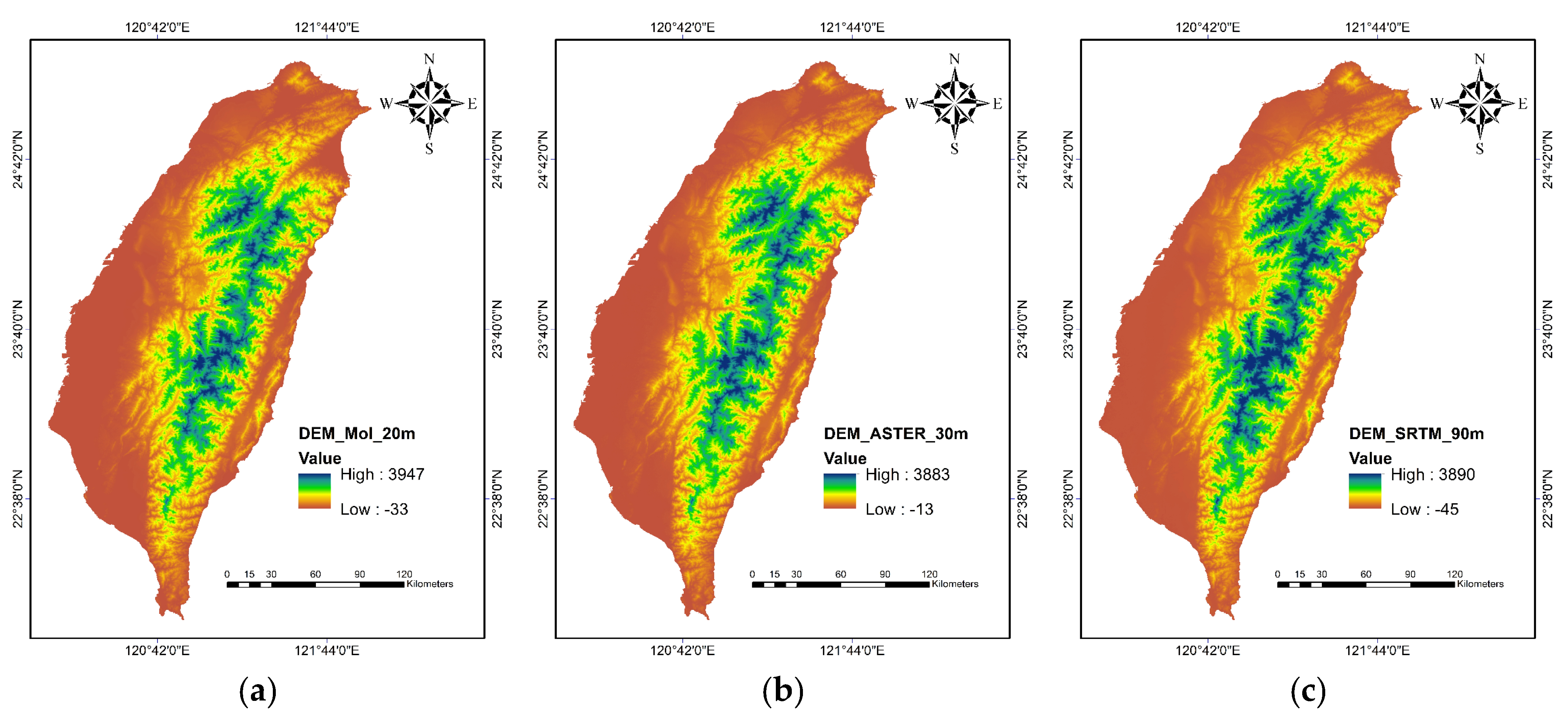
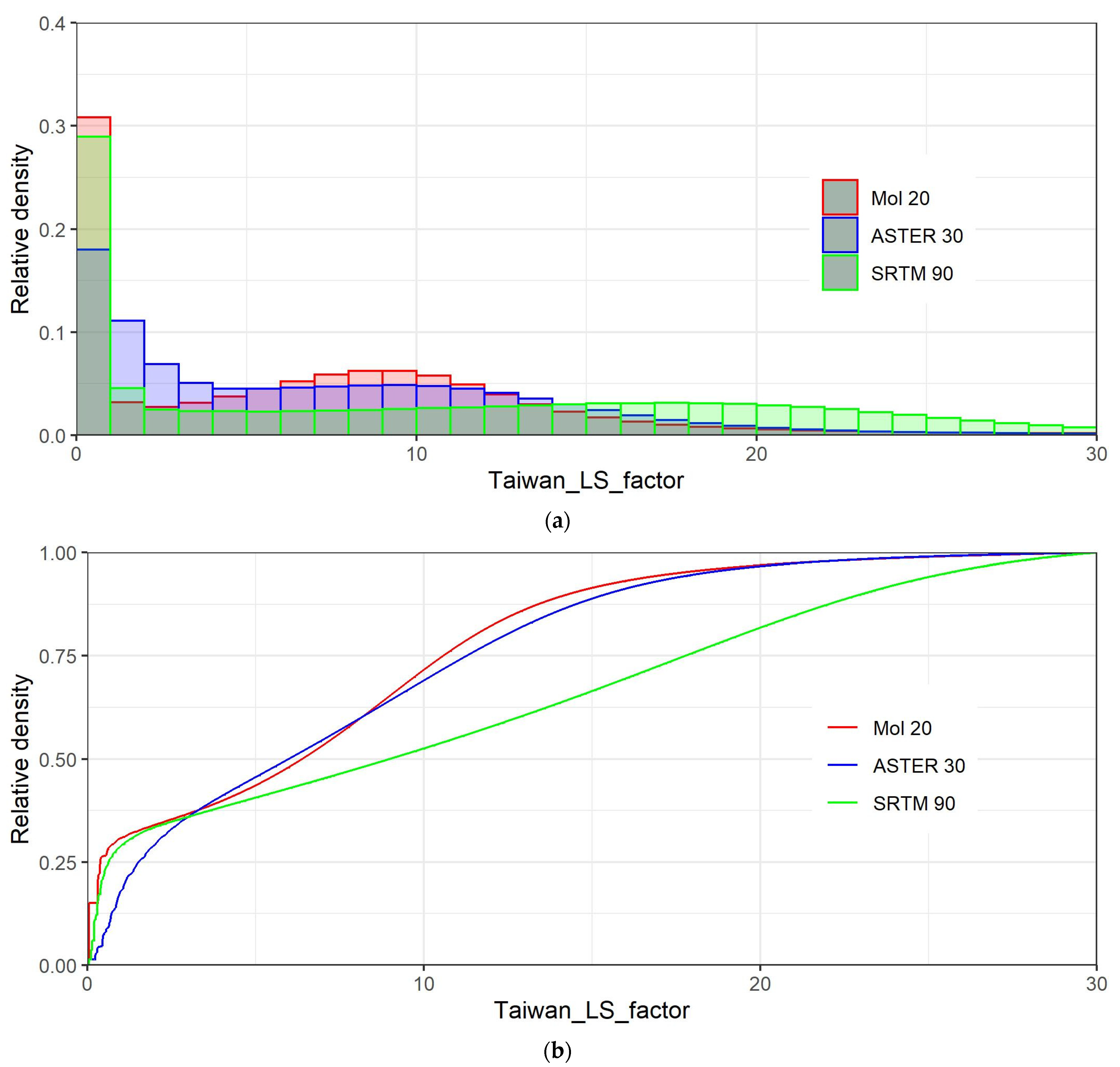
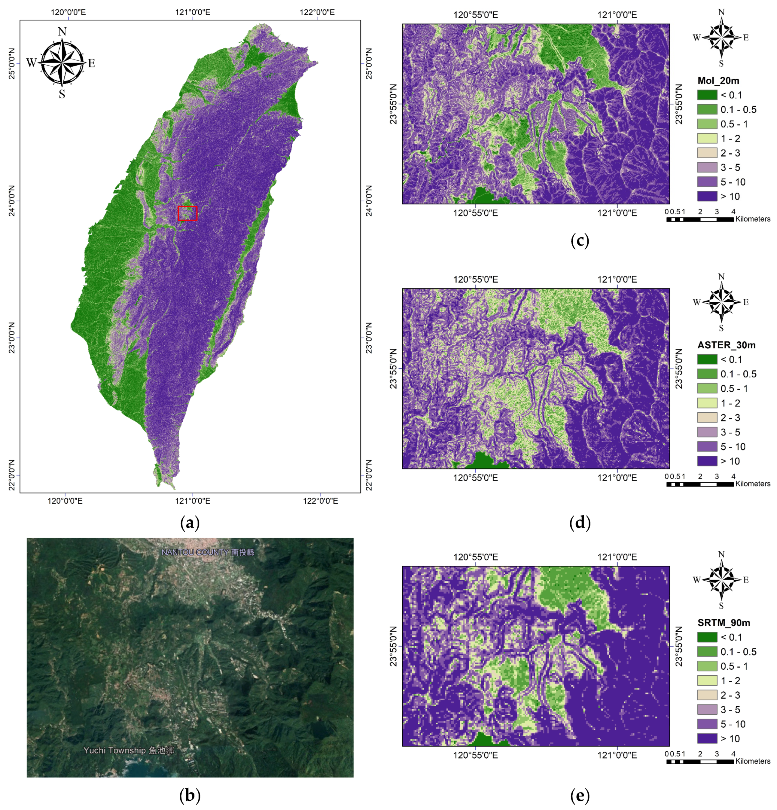
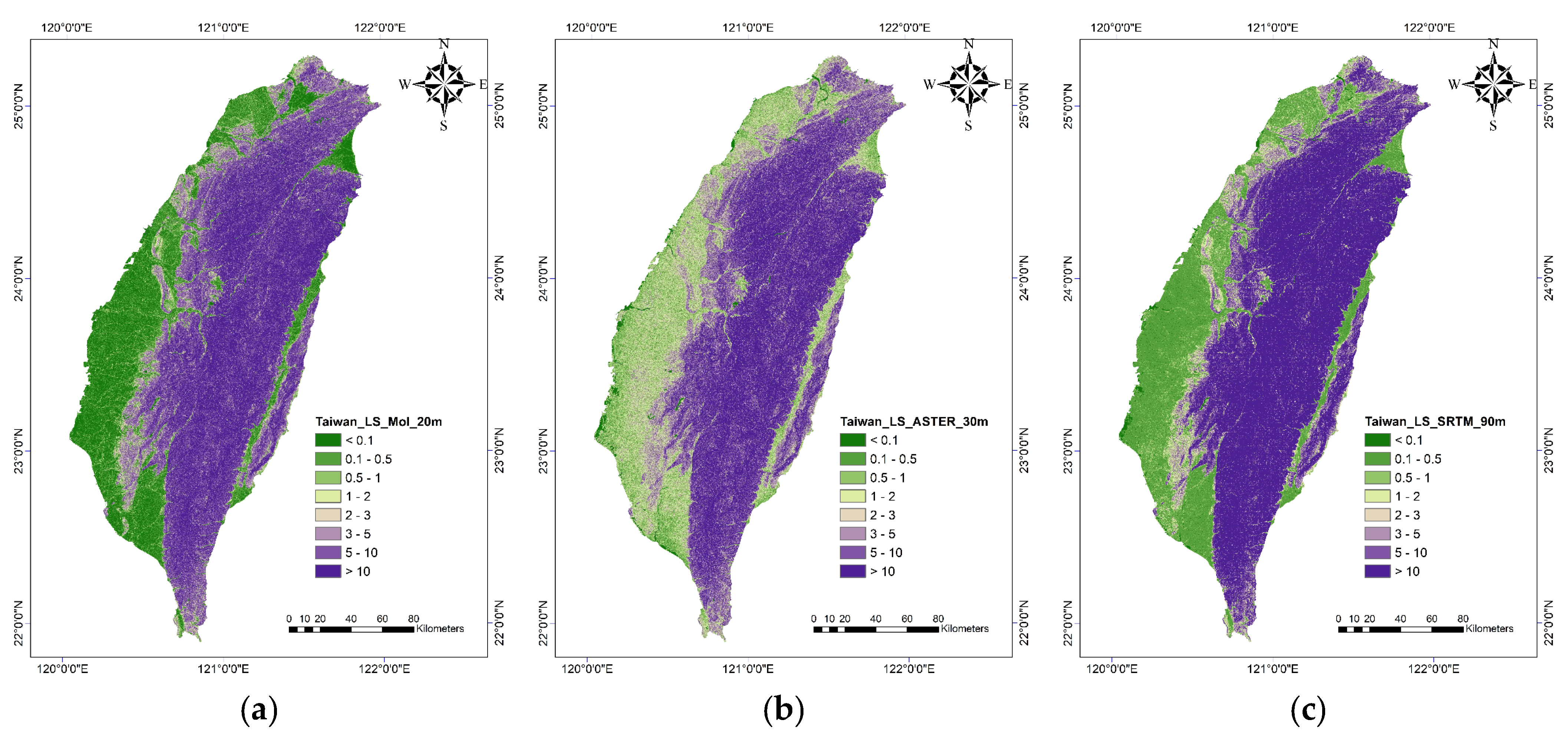
4.1. Comparison of Taiwan’s LS Factor Derived from Three DEMs

Figure 2 depicts the results of Taiwan’s LS factors using the same color scheme as that of Panagos et al. [4] for the EU, and

Table 2. The statistics of the LS factors of Taiwan and EU.

DEM	Cell Size (m)	Taiwan			EU
		Mean	Std	Coefficient of Variation	Mean	Std	Coefficient of Variation
MoI DEM	20	8.24	13.71	1.66	-	-	-
EU-DEM	25	-	-	-	1.95	4.28	2.19
ASTER DEM	30	7.63	7.73	1.01	2.84	3.72	1.31
SRTM DEM	90	10.77	9.80	0.91	-	-	-

provides the statistics of the LS factors. Following the classification of the LS factor of Panagos et al. [4], the LS factors were divided into eight classes (Figure 2). The figure shows that the LS factors greater than 3 (purple color) were primarily concentrated longitudinally in Taiwan’s central and eastern regions. Meanwhile, the population of Taiwan is concentrated in the west side of Taiwan, where the LS factors are smaller than one. When the grid size of DEMs varies in Taiwan, it is evident that the LS factor value changes as well. The mean LS factors do not reflect the hypothesis that the smaller the grid size, the larger the LS factor, as shown in Table 2. The mean LS factor of the ASTEM DEM is the smallest, while the mean LS factor of the SRTM DEM is the largest, and the mean LS factor of the MoI DEM lies in between the two extremes. In addition, the mean LS factors of the MoI and ASTER DEMs are close to each other, whereas the mean LS factor of the SRTM DEM is substantially higher.

The histograms of Taiwan’s LS factors, based on the three DEMs, are presented in Figure 3a. The tails of all three DEMs are lengthy. However, because the majority of the LS factors are on the lower end of the spectrum, we set an X-axis limit of 30 for presentation purposes. The histogram of the MoI DEM has the largest peak (between 0 and 1) and a characteristic and distinct second peak between 8 and 10. The ASTER and SRTM DEMs also have their peaks between 0 and 1; however, they do not have a recognizable second peak. Although the SRTM DEM lacks a noticeable second peak, its distribution is more spread out to the right than the other two DEMs. This is why the SRTM DEM has a greater mean LS factor than the other two DEMs.

If we look at the cumulative density distribution (CDF) of the LS factors (Figure 3b), we can see all three curves intersect at roughly LS = 3.1. Before 3.1, the MoI and SRTM DEMs have essentially identical curves, with the ASTER DEM’s curve underneath them. However, after 3.1, the MoI and ASTER curves are practically undistinguishable, and this time, the SRTM curve is consistent below them. This is a really intriguing find. Although the specific origin of this phenomenon is not known, it means that for flat areas with an LS smaller than 3.1 in Taiwan, the use of the MoI and SRTM DEMs to compute the LS factors and simulate soil erosion is likely to yield the same outcome. On the other hand, for hilly terrain with LS factors greater than 3.1, the use of MoI and ASTER to estimate the LS factors is projected to be equivalent if other issues raised below are not considered.

A location near the Yuchi Township in Nantou County was selected to further compare the different resolutions of the three DEMS in greater detail. Figure 4 shows their Google Earth image and LS factor distributions computed from the three DEMs. The local variation in the LS factors of the 90 m DEM is poorer than that of the 20 m and 30 m DEMs, as clearly observed in the figure. The cell size reflects the complicated topography of Taiwan, since it has many rough mountain areas with significant elevation changes within a short distance. As a result, as various researchers have pointed out [8,23], a complex terrain necessitates a finer grid size than for a simple terrain. The accuracy of LS factor computation decreases as the grid sizes become greater [8]. At intermediate resolutions, accuracy drops slightly, but at coarse resolutions, it drops substantially [23]. The 90 m DEM grid cells’ larger horizontal spacing of elevation points resulted in a loss of topographic information by smoothing out the landscape.

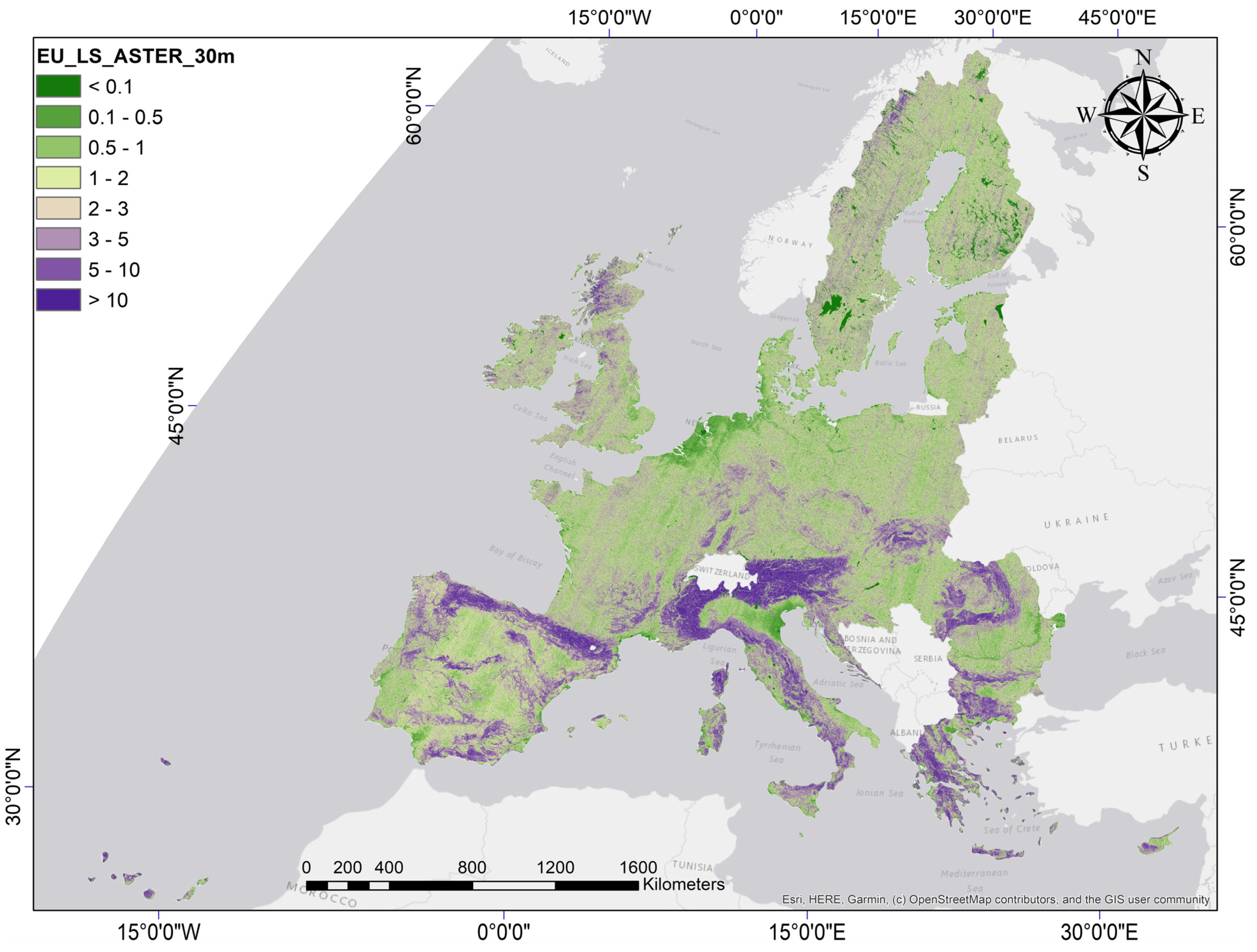
4.2. Comparison of Taiwan’s and EU’s LS Factors

Panagos et al. [4] calculated the LS factor using the 25 m EU-DEM of the European Union, a hybrid product of SRTM and ASTER. Taiwan, of course, is not included in the EU-DEM. Therefore, we used the global ASTER DEM in this study to compare Taiwan and the EU (and the United Kingdom, which left the EU on 31 January 2020). The SRTM DEM was not chosen because it did not cover the entirety of Europe. The results were previously shown in Table 2.

The result shows that the EU’s mean LS factor is 2.84, while Taiwan’s mean LS factor is 7.63. This demonstrates that, on average, Taiwan’s terrain is steeper and more rugged than that of the European Union. This is one of the reasons why soil erosion in Taiwan’s watersheds [11,12] is significantly higher than that of the EU average [3,24]. Using the ASTER DEM, Figure 5 depicts the distribution of the LS factor in the EU. Unlike Taiwan, the figure illustrates that most of the EU is covered in green rather than purple. To put it another way, the bulk of EU countries have low LS factors, whereas Taiwan has high LS factors. This creates a stark contrast in the undulation of the terrains and the resulting amounts of soil erosion.

Table 3. The mean LS factor of EU countries and the UK.

Country Name	Code	Mean	Standard Deviation	Coefficient of Variation
Austria	AT	6.95	7.94	1.14
Belgium	BE	1.43	1.51	1.05
Bulgaria	BG	3.46	3.91	1.13
Cyprus	CY	3.37	3.68	1.09
Czech Rep.	CZ	2.39	2.26	0.95
Germany	DE	2.12	2.35	1.11
Denmark	DK	1.26	1.13	0.90
Estonia	EE	1.76	1.55	0.88
Spain	ES	3.21	4.00	1.25
Finland	FI	1.84	1.61	0.87
France	FR	2.90	4.05	1.40
Greece	GR	4.98	5.15	1.03
Croatia	HR	3.04	3.26	1.07
Hungary	HU	1.75	1.64	0.94
Ireland	IE	2.37	2.22	0.94
Italy	IT	4.90	6.37	1.30
Lithuania	LT	1.87	1.54	0.83
Luxembourg	LU	2.56	2.46	0.96
Latvia	LV	1.84	1.46	0.80
Malta	MT	1.42	1.92	1.35
Netherlands	NL	0.64	0.66	1.04
Poland	PL	1.88	1.72	0.92
Portugal	PT	2.72	2.97	1.09
Romania	RO	3.29	3.74	1.14
Sweden	SE	2.24	2.13	0.95
Slovenia	SI	5.41	5.52	1.02
Slovakia	SK	3.96	3.76	0.95
United Kingdom	UK	2.70	2.69	0.99

shows the mean LS factor for each EU country and the United Kingdom. The average LS factor of Taiwan was previously shown in Table 2. The data show that Taiwan has a significantly higher mean LS factor than any of the UK and EU countries. Austria, Slovenia, and Greece have the greatest LS factors in the EU, and their values are the closest to Taiwan. Taiwan is, in some ways, a much warmer version of these countries.

5. Discussion and Conclusions

The LS factor quantifies topography’s effect on soil erosion, and the LS factor has the greatest impact on soil loss at the European level [4]. In this study, we employed three DEMs, including a high-resolution (20 m) DEM, to compute the LS factor in Taiwan using the Desmet and Govers [20] equation applied in SAGA GIS. This is the first study to construct a map of Taiwan’s LS factor without assuming a fixed slope length of 40 m [15] and using the European Union’s accepted upslope contributing area technique.

This research yielded a number of intriguing results. First, due to the widespread use of the USLE/RUSLE models, countries can compare the results of soil erosion analysis. When we determine the average rate of soil erosion in a region, the average of the products of five erosive factors is used (rainfall erosivity factor Rm, soil erodibility factor Km, topographic factor LS, cover-management factor C, and support practice factor P). According to Li et al. [25], with a maximum absolute error of 10.6% to 28.4% (depending on DEM and watershed), this average of products can be approximated by the product of averages as follows:

$$\frac{{{\displaystyle \sum }}_{i=1}^{n}R{m}_{i}K{m}_{i}L{S}_i{C}_i{P}_i}{n}\approx \frac{{{\displaystyle \sum }}_{i=1}^{n}R{m}_i}{n}\frac{{{\displaystyle \sum }}_{i=1}^{n}K{m}_i}{n}\frac{{{\displaystyle \sum }}_{i=1}^{n}L{S}_i}{n}\frac{{{\displaystyle \sum }}_{i=1}^n{C}_i}{n}\frac{{{\displaystyle \sum }}_{i=1}^n{P}_i}{n}$$

(7)

As an approximation, we may analyze specific erosive factors separately and compare them across areas and nations in order to determine their proportionate impact on total soil loss in various parts of the world.

Second, Taiwan’s mean LS factor, as calculated by Desmet and Govers [20] using the upslope contributing area, is extremely high. When compared to the EU, the high values are even more apparent. Taiwan’s LS factor is 2.69 times the EU average (7.63/2.84 = 2.69) and higher than any EU country, including the UK. In other words, when all other elements are held constant (rainfall erosivity factor, soil erodibility factor, cover-management factor, and support practice factor), the average soil erosion of Taiwan is around 2.69 times that of the EU. Austria has the highest mean LS factor among the EU countries and the UK, at 6.95, which is 91 percent of Taiwan’s. This indicates the importance of the LS factor in soil loss and echoes Taiwan’s high soil erosion rates as measured by erosion pins [26,27].

Third, using the ASTER DEM, the mean LS factors of EU nations determined in this work are larger than those published by Panagos et al. [4]. We think there are three possible causes for this disparity. First, unlike Panagos et al. [4], we did not apply a cutoff slope angle to the DEM. This is because we wanted to show a true geographical comparison between Taiwan and the European Union. Second, we used the most recent SAGA GIS version 8.1.1 and accepted the default values in the LS factor field-based module. Panagos et al. [4] did not provide the version number of their software or the options they used. We discovered that tinkering with the variables in SAGA GIS allowed us to generate vastly varied mean LS factors. Third, different DEMs were used in both studies. Even though the EU-DEM used by Panagos et al. [4] was based mostly on SRTM and ASTER, it is still not the same DEM as the ASTER DEM.

A fourth finding was, as expected, that the LS factor’s accuracy is highly dependent on the DEM resolution. However, large grid sizes may not always correspond to a lower topographic factor, which results in an underestimation of soil losses. In our study, although the LS factor was reduced from 8.24 to 7.63 when the cell size was increased from 20 to 25 m, it returned to 10.77 when the cell size was increased further to 90 m.

Finally, the MoI DEM’s LS factor distribution features a distinct second peak that is not visible in the ASTER or SRTM DEMs. Due to the fact that the 20 m MoI DEM was generated using airborne LiDAR, the second peak is unlikely to be the product of erroneous data. Furthermore, regardless of the DEM, the distribution of the LS factor always has a long tail. It is evident that the histograms offer more information and can be used to more accurately quantify a region’s topography than mean values alone. Their application deserves further examination.

To conclude, because USLE/RUSLE models are widely used, countries can compare the findings of soil erosion analyses. Due to the fact that soil loss is the multiplication of individual soil erosion factors based on rainfall, soil properties, topography, vegetation cover, and conservation measures, we may also investigate the individual factors independently and compare them across regions and nations to ascertain their relative influence on total soil loss in various parts of the world. This enables a more integrated worldwide effort to combat land degradation and promote the sustainable use of terrestrial ecosystems, amplifying their value.

References

1. Borrelli, P.; Alewell, C.; Alvarez, P.; Anache, J.A.A.; Baartman, J.; Ballabio, C.; Panagos, P. Soil erosion modelling: A global review and statistical analysis. Sci. Total Environ. 2021, 780, 146494. [Google Scholar] [CrossRef]
2. Bezak, N.; Mikoš, M.; Borrelli, P.; Alewell, C.; Alvarez, P.; Anache, J.A.A.; Panagos, P. Soil erosion modelling: A bibliometric analysis. Environ. Res. 2021, 197, 111087. [Google Scholar] [CrossRef] [PubMed]
3. Panagos, P.; Borrelli, P.; Poesen, J.; Ballabio, C.; Lugato, E.; Meusburger, K.; Montanarella, L.; Alewell, C. The new assessment of soil loss by water erosion in Europe. Environ. Sci. Policy 2015, 54, 438–447. [Google Scholar] [CrossRef]
4. Panagos, P.; Borrelli, P.; Meusburger, K. A new European slope length and steepness factor (LS-factor) for modeling soil erosion by water. Geosciences 2015, 5, 117. [Google Scholar] [CrossRef] [Green Version]
5. Khanifar, J.; Khademalrasoul, A. Multiscale comparison of LS factor calculation methods based on different flow direction algorithms in Susa Ancient landscape. Acta Geophys. 2020, 68, 783–793. [Google Scholar] [CrossRef]
6. Shan, L.; Yang, X.; Zhu, Q. Effects of DEM resolutions on LS and hillslope erosion estimation in a burnt landscape. Soil Res. 2019, 57, 797–804. [Google Scholar] [CrossRef]
7. Bircher, P.; Liniger, H.P.; Prasuhn, V. Comparing different multiple flow algorithms to calculate RUSLE factors of slope length (L) and slope steepness (S) in Switzerland. Geomorphology 2019, 346, 106850. [Google Scholar] [CrossRef]
8. Lu, S.; Liu, B.; Hu, Y.; Fu, S.; Cao, Q.; Shi, Y.; Huang, T. Soil erosion topographic factor (LS): Accuracy calculated from different data sources. Catena 2020, 187, 104334. [Google Scholar] [CrossRef]
9. Azizian, A.; Koohi, S. The effects of applying different DEM resolutions, DEM sources and flow tracing algorithms on LS factor and sediment yield estimation using USLE in Barajin river basin (BRB), Iran. Paddy Water Environ. 2021, 19, 453–468. [Google Scholar] [CrossRef]
10. Lo, K.F.A. Quantifying soil erosion for the Shihmen reservoir watershed, Taiwan. Agric. Syst. 1994, 45, 105–116. [Google Scholar] [CrossRef]
11. Chen, W.; Li, D.H.; Yang, K.J.; Tsai, F.; Seeboonruang, U. Identifying and comparing relatively high soil erosion sites with four DEMs. Ecol. Eng. 2018, 120, 449–463. [Google Scholar] [CrossRef]
12. Liu, Y.H.; Li, D.H.; Chen, W.; Lin, B.S.; Seeboonruang, U.; Tsai, F. Soil erosion modeling and comparison using slope units and grid cells in Shihmen reservoir watershed in Northern Taiwan. Water 2018, 10, 1387. [Google Scholar] [CrossRef] [Green Version]
13. Lin, B.S.; Chen, C.K.; Thomas, K.; Hsu, C.K.; Ho, H.C. Improvement of the K-factor of USLE and soil erosion estimation in Shihmen reservoir watershed. Sustainability 2019, 11, 355. [Google Scholar] [CrossRef] [Green Version]
14. Nguyen, K.A.; Chen, W.; Lin, B.S.; Seeboonruang, U.; Thomas, K. Predicting sheet and rill erosion of Shihmen reservoir watershed in Taiwan using machine learning. Sustainability 2019, 11, 3615. [Google Scholar] [CrossRef] [Green Version]
15. Lin, Y.C.; Huang, S.L. Spatial Emergy Synthesis of the Environmental Impacts from Agricultural Production System Change—A Case Study of Taiwan. In Proceedings of the 7th Biennial Emergy Research Conference, Gainesville, FL, USA, 12–14 January 2012. [Google Scholar]
16. Alexakis, D.D.; Hadjimitsis, D.G.; Agapiou, A. Integrated use of remote sensing, GIS and precipitation data for the assessment of soil erosion rate in the catchment area of “Yialias” in Cyprus. Atmos. Res. 2013, 131, 108–124. [Google Scholar] [CrossRef]
17. Ranzi, R.; Le, T.H.; Rulli, M.C. A RUSLE approach to model suspended sediment load in the Lo River (Vietnam): Effects of reservoirs and land use changes. J. Hydrol. 2012, 422–423, 17–29. [Google Scholar] [CrossRef]
18. Renard, K.G.; Foster, G.R.; Weesies, G.A.; McCool, D.K.; Yoder, D.C. Predicting Soil Erosion by Water: A Guide to Conservation Planning with the Revised Universal Soil Loss Equation (RUSLE), Agricultural Handbook Number 703; United States Department of Agriculture: Washington, DC, USA, 1997.
19. Foster, G.R.; Wischmeier, W.H. Evaluating Irregular Slopes for Soil Loss Prediction. Trans. Am. Soc. Agric. Eng. 1974, 17, 305–309. [Google Scholar] [CrossRef]
20. Desmet, P.J.J.; Govers, G. A GIS procedure for automatically calculating the USLE LS factor on topographically complex landscape units. J. Soil Water Conserv. 1996, 51, 427–433. [Google Scholar]
21. Conrad, O.; Bechtel, B.; Bock, M.; Dietrich, H.; Fischer, E.; Gerlitz, L.; Wehberg, J.; Wichmann, V.; Boehner, J. System for Automated Geoscientific Analyses (SAGA) v. 2.1.4. Geosci. Model Dev. 2015, 8, 1991–2007. [Google Scholar] [CrossRef] [Green Version]
22. Molnár, D.K.; Julien, P.Y. Estimation of upland erosion using GIS. Comput. Geosci. 1998, 24, 183–192. [Google Scholar] [CrossRef]
23. Gao, J. Resolution and accuracy of terrain representation by grid dems at a micro-scale. Int. J. Geogr. Inf. Sci. 1997, 11, 199–212. [Google Scholar] [CrossRef]
24. Panagos, P.; Ballabio, C.; Himics, M.; Scarpa, S.; Matthews, F.; Bogonos, M.; Borrelli, P. Projections of soil loss by water erosion in Europe by 2050. Environ. Sci. Policy 2021, 124, 380–392. [Google Scholar] [CrossRef]
25. Li, J.-Y.; Yang, K.-J.; Chen, W. Approximation equation of erosion calculation in GIS. In Proceedings of the 37th Asian Conference on Remote Sensing, ACRS, Colombo, Sri Lanka, 17–21 October 2016; Volume 3, pp. 1837–1843. [Google Scholar]
26. Nguyen, K.A.; Chen, W.; Lin, B.S.; Seeboonruang, U. Comparison of Ensemble Machine Learning Methods for Soil Erosion Pin Measurements. ISPRS Int. J. Geo-Inf. 2021, 10, 42. [Google Scholar] [CrossRef]
27. Nguyen, K.A.; Chen, W. DEM-and GIS-Based Analysis of Soil Erosion Depth Using Machine Learning. ISPRS Int. J. Geo-Inf. 2021, 10, 452. [Google Scholar] [CrossRef]
Figure 1. The DEMs of Taiwan: (a) MoI DEM (20 m), (b) ASTER V3 (30 m), (c) SRTM V4.1 (90 m).
Sustainability 14 03059 g001
Figure 2. Taiwan’s LS factors: (a) MoI DEM (20 m), (b) ASTER V3 (30 m), (c) SRTM V4 (90 m).
Sustainability 14 03059 g002
Figure 3. The distributions of Taiwan’s LS factors: (a) histograms and (b) cumulative distribution curves.
Sustainability 14 03059 g003
Figure 4. A location near the Yuchi Township in Nantou County was selected for comparison: (a) location, (b) Google Earth image, (c) 20 m DEM, (d) 30 m DEM, and (e) 90 m DEM.
Sustainability 14 03059 g004
Figure 5. The LS factors of the EU (ASTER DEM).
Sustainability 14 03059 g005