Monitoring of Soil Salinization in the Keriya Oasis Based on Deep Learning with PALSAR-2 and Landsat-8 Datasets

Abstract

Currently, soil salinization is one of the main forms of land degradation and desertification. Soil salinization not only seriously restricts the development of agriculture and the economy, but also poses a threat to the ecological environment. The main purpose of this study is to map soil salinity in Keriya Oasis, northwestern China using the PALSAR-2 fully polarized synthetic aperture radar (PolSAR) L-band data and Landsat-8-OLI (OLI) optical data combined with deep learning (DL) methods. A field survey is conducted, and soil samples are collected from 20 April 2015 to 1 May 2015. To mine the hidden information in the PALSAR-2 data, multiple polarimetric decomposition methods are implemented, and a wide range of polarimetric parameters and synthetic aperture radar discriminators are derived. The radar vegetation index (RVI) is calculated using PALSAR-2 data, while the normalized difference vegetation index (NDVI) and salinity index (SI) are calculated using OLI data. The random forest (RF)-integrated learning algorithm is used to select the optimal feature subset composed of eight polarimetric elements. The RF, support vector machine, and DL methods are used to extract different degrees of salinized soil. The results show that the OLI+PALSAR-2 image classification result of the DL classification was relatively good, having the highest overall accuracy of 91.86% and a kappa coefficient of 0.90. This method is helpful to understand and monitor the spatial distribution of soil salinity more effectively to achieve sustainable agricultural development and ecological stability.

1. Introduction

As a form of soil degradation, soil salinization not only destroys resources and reduces agricultural production, but also poses a severe threat to the biosphere and ecological environment, thus becoming an environmental problem worldwide [1,2]. Soil salinization is a process during which soluble salt accumulates on the soil surface, and it is one of the main forms of land desertification and degradation [3].

According to statistics, approximately 8.31 million km² of soil in the world has been harmed by salinization [4]. More than 3% of soil resources are affected by salt [5]. China has been one of the countries with severe salinization problems [6]. China alone is covered by 10% of the world’s salinized land area [7,8], and Xinjiang is one of the largest saline soil distribution areas [9], accounting for 36.8% of the country’s saline-alkali land area, mainly distributed in the oasis-desert ecosystem in southern Xinjiang (nearly 50%) [10]. Therefore, realizing large-scale, high-precision soil salinization monitoring and scientific prediction of salinization risks and hazards are fundamental to alleviating environmental pressure.

Salinity monitoring based on the traditional methods requires frequent sampling, which can be cost-prohibitive [11]. Remote sensing technology has been increasingly used in salinity monitoring due to its advantages of wide coverage, short cycle time, and high accuracy [12]. Optical remote sensing has played an important role in regional and global soil salinization monitoring, mapping, and prevention [13]. However, it is difficult to interpret images under unstable weather conditions, and images are typically collected during the day, so the image collection period is limited [14]. A synthetic aperture radar (SAR) can obtain information under all conditions and can penetrate clouds and near-surface soil profiles, providing an effective tool for ground observation and timely extraction of salinized soil information [13,14,15,16,17]. Additionally, SAR data have been proven to be effective for the extraction of salinity information, due to dielectric properties that are sensitive to soil salinity; soil salinity is also a key factor to electrical conductivity [18,19]. A polarimetric synthetic aperture radar (PolSAR) is a multi-channel, multi-parameter radar system that can collect images under different weather conditions for 24 h [20]. Compared with the traditional single-polarization synthetic aperture radar data, PolSAR data can provide full-polarization scattering information on the target ground object [21], and the scattering characteristics of different ground objects can be expressed in the form of vectors to the greatest extent, thereby revealing the scattering of ground objects’ difference [22].

The polarimetric parameters extracted by different polarimetric target decomposition methods are intensely important because they are related to the physical characteristics of ground objects [13], and therefore may be applied to classify and map soil salinization [23]. The subject of the polarimetric decomposition of a target has received great attention and achieved rapid development because it can reveal the scattering mechanism of the target and enhance the understanding of the target’s scattering characteristics [24,25]. In addition, its polarization feature decomposition provides an effective tool for microwave remote sensing in the processes of saline land information extraction and salinity dynamics monitoring and can provide timely and effective guidance on agricultural production practices in arid areas [26]. Accordingly, the application degree and field of PolSAR images have been and are continuously expanding, and various corresponding image interpretation technologies have been developing rapidly [27]. In the past two decades, optical and PolSAR data with different spectral, temporal, and spatial resolutions have been widely used to describe the severity of soil salinization [28].

To improve the quality of soil salinity mapping, several machine learning algorithms were used in combination with radar data. Xie, et al. [29], using Sentinel-1 data combined with the random forest (RF) method to extract the distribution range of different land uses and finally verify the extraction accuracy of flue-cured tobacco planting. Nurmemet et al. [23] reported that a wrapper-based support vector machine can be used together with PolSAR data for soil salinity mapping in semi-arid areas. In a new study, Taghadosi et al. [30] showed that soil salinity mapping is viable for semi-arid areas, along with the use of Sentinel-1 SAR data (VV, VH, and their derived texture) and support vector regression.

Recently, Deep Learning (DL) based methods have achieved promising results in a multitude of fields, including the vision of computers [31], the theory of information [32], and the processing of natural language [33]. In the last few years, DL has also achieved great success in PolSAR data classification [34]. Zhou et al. applied CNN to PolSAR image classification for the first time [35]; in their work, a three-layer architecture was introduced to classify PolSAR images and obtained promising classification results. Jiang et al. [36] extended the CNN application to recognize the target in SAR images. Zhang, et al. [37] proposed a novel object-based convolutional neural network (OCNN) for urban land use classification using VFSR images. Ndikumana et al. [38] took advantage of RNN to deal with the agricultural classification study with multitemporal Sentinel-1 SAR data.

As a part of machine learning, DL can process composite data efficiently, and has a strong feature extraction capability [39]. Generally DL can provide better classification results than the traditional classifiers [40].

The ultimate goal of this research is to monitor soil salinization in the Keriya River basin, Xinjiang, China, using DL methods with PALSAR-2 data and OLI data.

2. Materials and Methods

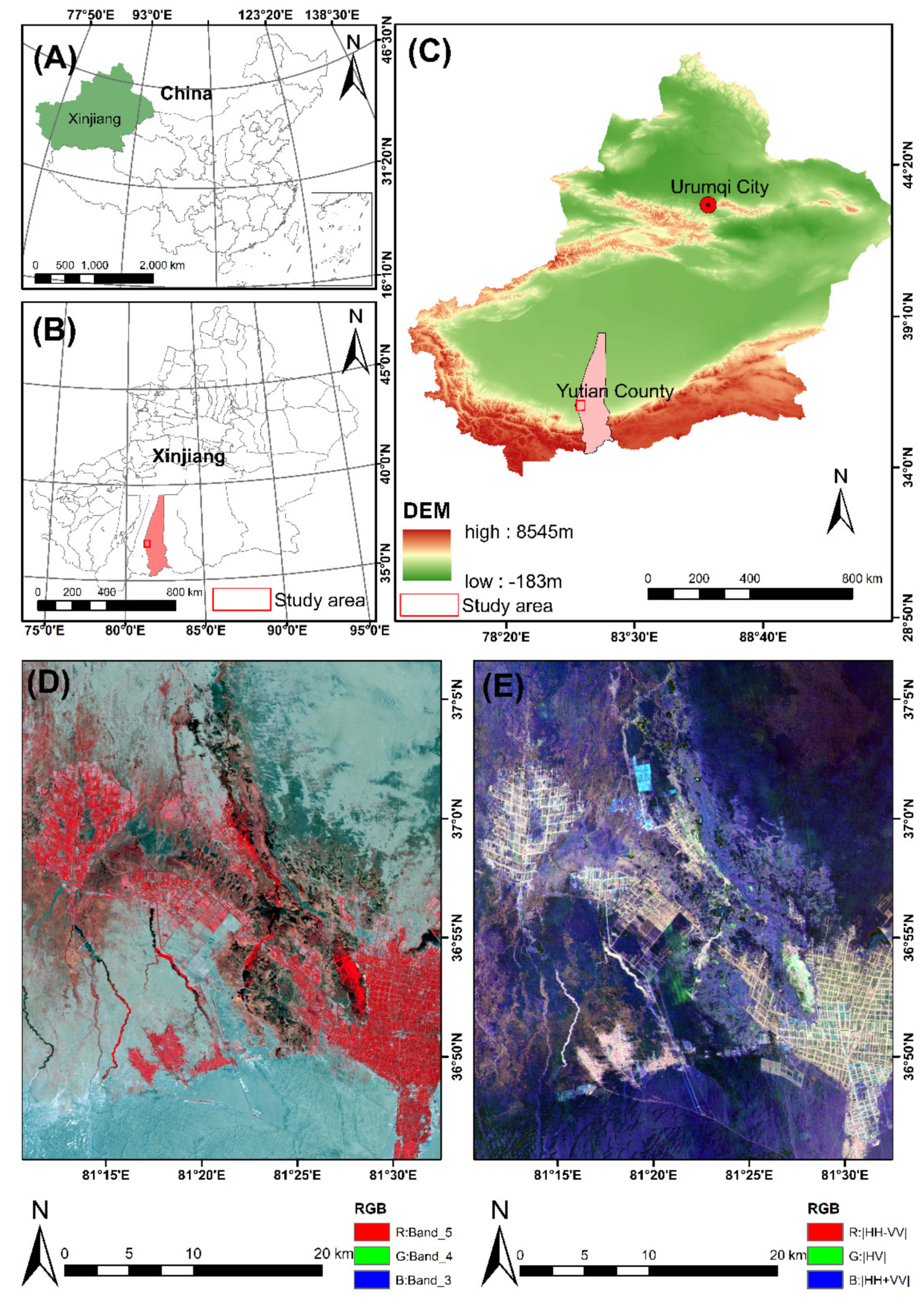
2.1. Study Area

The study site is the Keriya Oasis in the Tarim Basin, Xinjiang, China (35°14′–39°29′ N, 81°09′ E–82°51′ E), as shown in Figure 1. The research area is located at the southern edge of Taklimakan Desert and the central northern slope of Kunlun Mountain, which is a typical oasis-desert intersection with an altitude of 1180~5460 m [23].

The study site has a temperate continental climate, with perennial drought and large daily temperature difference. The lowest average temperature in January is −5.8 °C and the highest average temperature in July is 25 °C. The local area is rare, and the average annual precipitation is 44.7 mm [41]. The average evaporation rate is 2498 mm, the evaporative rainfall ratio is approximately 55:1, and the frost-free period is approximately 200d [41]. The vegetation coverage of the oasis on the middle and north slope of Kunlun Mountain is 10% Mt. 40%. The plants studied are mainly desert species, such as Phragmites australis, Tamarix chinensis, Populus euphratica, Alhagi sparsifolia, Karelina caspica and Kalidium gracile [42].

Keriya River originates from the Kunlun Mountains, flows through the Keriya Oasis, and after approximately 700 km ends in the hinterland of the Taklimakan Desert [43]. The river is primarily supplied by glacial melt, snowmelt, and precipitation in the Kunlun Mountains [44]. The movement of dissolved salts to the land surface is facilitated by a combination of hyper-arid climate, topographic conditions, and shallow groundwater level [45]. This leads to soil salinization and desertification, especially in the transition belt between oasis and desert [43,44,45]. Therefore, intensive understanding and timely monitoring of the spatial distribution of soil salinity have been paramount tasks for both agricultural sustainability and ecological stability [45].

2.2. Data

2.2.1. Remote Sensing Data

The advanced Land Observing Satellite-2 (ALOS-2) is a Japanese earth observation satellite that was launched on May 24, 2014 [46]. PALSAR-2 (Phased Array type L-band synthetic aperture radar) sensor in L-band (1.2 GHz band), maximum resolution of 3 m × 1 m (distance direction × azimuth direction), two polarization modes horizontal (H) and vertical (V), and different scattering elements (HH, HV, VH, VV) for sensitivity to different features of ground target features helps to identify different land types, under various weather conditions [47]. Compared with other single-polarization and dual-polarization SAR data, PALSAR-2 has a higher resolution, a larger observation range, shorter revisit period, clearer texture features of the ground features, richer imaging modes, and a better data transmission capability, and plays a greater role in mapping, regional observation, disaster monitoring, and resource investigation [48,49].

In this study, fully polarized PALSAR-2 data (including HH, HV, VV, and VH polarization modes) were acquired on 23 April 2015, on a descending orbit in quad-pol strip mode at an incident angle of 30.4°. Specific parameters about the PALSAR-2 data are given in

Table 1. Main parameters of fully Polarimetric PALSAR-2 data.

Parameter	Value
Data Observation Date	23 April 2015
Map Projection	UTM
Polarization	HH, HV, VH, VV
Product Type	HBQ
Operating Band	L band (1.2 GHz)
Satellite altitude	628 km
Incident angle	30.4°
Processing level	L1.1
Operation mode	SM2
Observation mode	Strip map (High-sensitive Quad)
Observation and orbit direction	Right, Ascending
File format	CEOS SAR
Swath	40–50 km × 70 km (Range × Azimuth)
Nominal resolution	5.1 × 4.3 m (Range × Azimuth)
Orbit path, frame	158,730

. The Landsat-8-OLI (OLI) image acquired on 28 May 2015, is displayed in Figure 1D.

The PALSAR-2 data in CEOS mode at level 1.1 in the study area were preprocessed using remote sensing processing software SNAP 7.0 provided by the European Space Agency (ESA). The tasks performed were as follows: (1) generating a single look complex (SLC) image; (2) multi-looking was performed using 4 × 2 looks in the range and azimuth, respectively, generating power image; (3) speckle filtering was performed using the refined Lee filter with the window size of 5 × 5, and noise reduction [50]; (4) geocoding and radiometric calibration [51,52], using a shuttle radar topography mission (SRTM), digital elevation model (DEM), and radiometric normalization, (i.e., modified cosine model) [53]; (5) geo-referencing to the Universal Transverse Mercator (UTM) coordinate system, Zone 44 North with the World Geodetic System Datum of 1984 (WGS84); (6) data resampling, image resizing to the optimal image resolution of 20 m × 20 m. The processing flow is shown in Figure 2. After data preprocessing, the backscatter coefficient (σ) in dB is generated. The statistical characteristics of the backscatter coefficient for each polarization band are shown in

Table 2. Backscattering statistical characteristics of PALSAR-2 data.

Number	Polarization	Statistical Value of Backscattering Coefficient (dB)
		Minimum	Maximum	Average	Standard Deviation
1	HH	−50.415756	9.823721	−17.312596	4.936925
2	HV	−50.720654	2.014654	−21.489555	5.107262
3	VH	−51.055477	2.264093	−26.473120	5.106566
4	VV	−52.791847	9.967834	−16.671018	4.556887

[23].

Landsat-8 is a satellite jointly developed and manufactured by NASA and USGS for medium resolution observations of the globe. The Landsat-8-OLI (OLI) has nine bands for effective monitoring of soil salinization [54,55]. In this paper, OLI images were preprocessed by ENVI 5.3^® software, including radiometric calibration, atmospheric correction, resampling, and clipping; finally, the image registration of PALSAR-2 data was performed based on the Landsat-8-OLI image. The OLI image acquired on 28 May 2015 is displayed in Figure 1D.

2.2.2. Field Data

In this study, field sampling was conducted in the period from 20 April 2015 to 1 May 2015. According to the field survey results and the specific field conditions of the study area, the land cover types of the study area can be divided into six categories: vegetation, water, strongly salinized soil, moderately salinized soil, slightly salinized soil, and bare land, as demonstrated in Figure 3.

When arranging soil sampling points in the field, the unity of pixels and the factors of vegetation type were considered, and a flat plot with a single soil type and a single feature of approximately 20 m² were used for sampling. After the soil sampling from the soil surface (0–10 cm), the soil physical and chemical characteristics such as soil salinity were measured in the laboratory. The sample preparation process included the following steps. First, soil samples were air-dried and sieved through 1-mm sieves. Next, the soil sample was mixed in a flask with distilled water at a ratio of 1:5; the flask was shaken manually for three minutes to allow the soil to infiltrate fully. Then, the fully mixed solution was left to stand for 30 min. Finally, when the solution became clear, the solution was filtered, and the total soluble salts were measured. In this process, the electrical conductivity of the soil water extract was measured (in ms/cm), and the total soluble salt content (g/kg) was calculated by the regression equation of EC. Different degrees of salinization (i.e., strongly, moderately, and slightly saline soils) were determined based on the surface soil salt concentration, groundwater table, and vegetation coverage, as shown in Figure 3 and

Table 3. LCLU classes with varying severity of soil salinization, characteristics, and their training and validation groups in the Keriya Oasis.

Symbol	Class	Characteristics	Training		Validation
			Plots	Pixels	Plots	Pixels
WB	Water Body	River, pond, swamp, lake	32	4928	28	4312
VG	Vegetation	Red willow, poplar, camel thorn, pike, grass, crops	50	7700	42	6468
BL	Barren land	Gobi, desert, rocky ground	41	6314	38	5855
HS	Strongly salinized soil	EC value 4–8 (dsm−1), salt crust is 2–10 cm, water table depth is 0.5–1.5 m, barren land with vegetation coverage less than 5%	44	7040	42	6720
MS	Moderately Salinized soil	EC value 4–6 (dsm−1), salt crust of 1–4 cm, water table depth is 1–2 m, vegetation coverage of around 5%–15%	41	6519	40	6360
SS	Slightly Salinized Soil	EC value 2–4 (dsm−1), with thin salt crust (around 0–2 cm), water table depth is 1.4–3 m, vegetation coverage of around 30%	39	6162	41	6519

.

Combined with a number of photo libraries collected from field trips and OvitalMap^® (https://www.ovital.com, accessed on 1 May 2015) high-resolution images, a total of 478 sample plots were collected for image classification and accuracy evaluation; 247 were used as training data, and the remaining 231 were used as verification data. To ensure that samples were evenly distributed throughout the study area, each land cover category contained at least 28 samples, and each sample contained approximately 150 pixels, as shown in Table 3.

2.3. Methods

Figure 4 illustrates the process workflow of this research, which is detailed in the following sections.

2.3.1. Polarimetric Decomposition

The theorem of target polarimetric decomposition was first proposed by Huynen [56] in 1970, and after nearly 50 years of development, various polarimetric decomposition methods have been proposed [57]. Target decomposition is an important method in the analysis of polarized SAR data. This method decomposes the complex scattering process into several single scattering components with the corresponding scattering matrices [58].

Coherent decomposition methods of scattering matrices denote an important class of decomposition algorithms in the field of target decomposition. The main element of this class of methods is the representation of a scattering matrix as a product or a sum of elementary scattering matrices that can be interconnected with a particular scattering mechanism [59]. Pauli matrices are obtained by the polarization scattering matrix $S$ decomposition, where different polarization basis matrices are defined, and the extraction of polarization features is performed, each representing a different type of feature [60]. The basic scattering matrix $S$ expressed in Pauli from given by:

$$S=\left[\begin{array}{ll}{S}_{\mathrm{HH}}\hfill & S_{\mathrm{HV}}\hfill \\ S_{\mathrm{VH}}\hfill & S_{\mathrm{VV}}\hfill \end{array}\right]=\frac{a}{\sqrt{2}}\left[\begin{array}{cc}1& 0\\ 0& 1\end{array}\right]+\frac{b}{\sqrt{2}}\left[\begin{array}{cc}1& 0\\ 0& -1\end{array}\right]+\frac{c}{\sqrt{2}}\left[\begin{array}{cc}1& 0\\ 0& 1\end{array}\right]+\frac{d}{\sqrt{2}}\left[\begin{array}{cc}1& -j\\ j& 1\end{array}\right]$$

(1)

where, $S_{\mathrm{HH}}$ and $S_{\mathrm{VV}}$ denote the co-polarization components; $S_{\mathrm{HV}}$ and $S_{\mathrm{VH}}$ are the cross-polarization components; and $a$, $b$, $c$, and $d$ are complex numbers and represent the weights of the scattering matrix on the four bases, and they are respectively calculated by:

$$a=\frac{S_{\mathrm{HH}}+S_{\mathrm{VV}}}{\sqrt{2}},b=\frac{S_{\mathrm{HH}}-S_{\mathrm{VV}}}{\sqrt{2}},c=\frac{S_{\mathrm{HV}}+S_{\mathrm{VH}}}{\sqrt{2}},d=j\frac{S_{\mathrm{HV}}-S_{\mathrm{VH}}}{\sqrt{2}}$$

(2)

Scattering matrix $S$ in the Pauli decomposition is vectorized on the basis of the target’s specific eigenvector $K$, which is given by:

$$K=\left[\begin{array}{llll}a\hfill & b\hfill & c\hfill & d\hfill \end{array}\right]\frac{1}{\sqrt{2}}{\left[\begin{array}{cccc}{S}_{\mathrm{HH}}+S_{\mathrm{VV}}& S_{\mathrm{HH}}-S_{\mathrm{VV}}& S_{\mathrm{HV}}+S_{\mathrm{VH}}& i\left(S_{\mathrm{VH}}-S_{\mathrm{HV}}\right)\end{array}\right]}^{\mathrm{T}}$$

(3)

when the reciprocity condition $S_{\mathrm{HV}}=S_{\mathrm{VH}}$ is satisfied, Equation (4) can be re-written as follows:

$$K=\left[\begin{array}{ccc}a& b& c\end{array}\right]=\frac{1}{\sqrt{2}}\left(\begin{array}{ccc}{S}_{\mathrm{HH}}+S_{\mathrm{VV}}& S_{\mathrm{HH}}-S_{\mathrm{VV}}& S_{\mathrm{HV}}+S_{\mathrm{VH}}\end{array}\right)$$

(4)

where, $K$ denotes the polarization eigenvector obtained by the Pauli decomposition. The physical meaning of the first term in the Pauli decomposition vector denotes single scattering, the second term denotes dihedral angular scattering where the radar and target center line of sight coincide with the normal dihedral plane, and the third term is related to multiple scattering.

A 3 × 3 apparent coherence matrix $T_3$ and a covariance matrix $C_3$ are respectively defined by:

$$\begin{array}{cc}{T}_3& =\left[\begin{array}{ccc}{T}_{11}& T_{12}& T_{13}\\ T_{12}^{*}& T_{22}& T_{23}\\ T_{13}^{*}& T_{23}^{*}& T_{33}\end{array}\right]\hfill \\ & =\frac{1}{2}\left[\begin{array}{c}<{\left|S_{hh}+S_{vv}\right|}^2><{\left(S_{hh}+S_{vv}\right)\left(S_{hh}-S_{vv}\right)}^{\mathrm{*}}>2<\left(S_{hh}+S_{vv}\right)S_{hv}^{*}>\\ <{\left(S_{hh}-S_{vv}\right)\left(S_{hh}+S_{vv}\right)}^{\mathrm{*}}><{\left|S_{hh}-S_{vv}\right|}^2>2<\left(S_{hh}-S_{vv}\right)S_{hv}^{*}>\\ 2<{S_{hh}\left(S_{hh}+S_{vv}\right)}^{\mathrm{*}}>2<{S_{hh}\left(S_{hh}-S_{vv}\right)}^{\mathrm{*}}>4<{\left|S_{hv}\right|}^2>\end{array}\right]\hfill \end{array}$$

(5)

$$\begin{array}{cc}{C}_3& =\left[\begin{array}{ccc}{C}_{11}& C_{12}& C_{13}\\ C_{12}^{*}& C_{22}& C_{23}\\ C_{13}^{*}& C_{23}^{*}& C_{33}\end{array}\right]\hfill \\ & =\left[\begin{array}{ccc}<{\left|S_{hh}\right|}^2>& \sqrt{2}<S_{hh}{S}_{hv}^{*}>& <S_{hh}{S}_{vv}^{*}>\\ \sqrt{2}<S_{hv}{S}_{hh}^{*}>& 2<{\left|S_{hv}\right|}^2>& \sqrt{2}<S_{hv}{S}_{vv}^{*}>\\ <S_{vv}{S}_{hh}^{*}>& \sqrt{2}<S_{vv}{S}_{hv}^{*}>& <{\left|S_{vv}\right|}^2>\end{array}\right]\end{array}$$

(6)

where, * denotes conjugate, |−| denotes mode, <·> denotes time or space set average [61].

The polarimetric decomposition is based on the scattering matrix, coherent matrix, or covariance matrix of a radar target or a covariance matrix of the radar target.

In this paper, the scattering matrix $S$, coherence matrix $T_3$, and covariance matrix $C_3$ of the PALSAR-2 data are calculated. To make the full use of the polarization feature information of PALSAR-2 data, polarization decomposition methods such as those of Cloude [62], Freeman [63], H/A/Alpha [64], Freeman Durden [65], Sinclair [66], Van Zyl [67], and Yamaguchi [68] are used in addition to the Pauli decomposition, as shown in

Table 4. Polarimetric features extracted from PALSAR-2 data.

Feature	Parameter Description	Symbols	Number of Parameters	Polarimetric Parameter
Original features	Scattering matrix elements	$S$	3	S11, S12, S21
	Coherency matrix elements	$T_3$	6	T11, T22, T33, T44, T55, T66
	Covariance matrix elements	$C_3$	3	C11, C22, C33
	Backscatter coefficient	HH,HV,VH,VV	4	hh,hv,vh,vv
Polarization decomposition parameters	Pauli	pauli	3	Pauli_r, Pauli_g, Pauli_b
	Cloude	Cloude	3	Cloude_dbl_r, Cloude_vol_g, Cloude_surf_b
	Freemen	Freemen	3	Freeman_dbl_r, Freeman_vol_g, Freeman_surf_b
	H/A/Alpha	H/A/α	3	Entropy, Anisotropy, alpha
	Freeman Durden	Freeman	3	Freeman Durden_dbl_r, Freeman Durden_vol_g, Freeman Durden_surf b
	Sinclair	Sinclair	3	Sinclair_r, Sinclair_g, Sinclair_b
	Vanzyl	VZ	3	VanZyl_dbl_r, VanZyl_vol_g, VanZyl_surf_b
	Yamaguchi	Yam	4	Yamaguchi_dbl_r, Yamaguchi_vol_g, Yamaguchi_surf_b, Yamaguchi_hlx
SAR discriminators	Radar vegetation index	RVI	1	rvi

. The energy information received by the SAR system reflected the scattering characteristics of the ground feature [69]. The Cloude, Pauli, Freeman, H/A/Alpha, Freeman Durden, Sinclair, Van Zyl, and Yamaguchi methods were used to calculate surface, volume, and double scattering values [70]. In the urban area, the polarization characteristic component is also dominated by double scattering. In our study area, the double scattering mainly reflects the road information [71], and the surface scattering is mainly the surface backscattering information, excluding the influence of vegetation [8]; the vegetation area is dominated by volume scattering [71]. The change information of surface vegetation in arid areas can better reflect the regional salinization [72].

2.3.2. Calculate the NDVI, SI and RVI

To extract the salinization information on the study area effectively, the normalized difference vegetation index (NDVI) and salinity index (SI) of the OLI data were calculated.

The normalized difference vegetation index ($NDVI$) [73] was calculated by:

$$NDVI=\frac{NIR-R}{NIR+R}$$

(7)

where,$NIR$ denotes near-infrared band reflectance, and $R$ denotes red band reflectance.

The salinity index ($SI)$ [74] was obtained using the reflectance OLI data band 1 ($B1$) and band 3 ($B3$) as follows:

$$Salinity Index\left(SI\right)=\sqrt{B1\times B3}$$

(8)

The radar vegetation index ($RVI$) can characterize the scattering stochasticity [75], and in this study, it was used to describe the canopy characteristics of vegetation. The specific calculation formula of $RVI$ is as follows:

$$RVI=\frac{4 \min {\left({\lambda }_1,{\lambda }_2,{\lambda }_3\right)}_{}}{{\lambda }_1+{\lambda }_2+{\lambda }_3}$$

(9)

where, λ₁, λ₂ and λ₃ are the eigenvalues of the covariance/coherency matrix.

2.3.3. Machine Learning Algorithms Used

Feature Selection from PALSAR-2 Imagery

Based on the full-polarization SAR image classification, the selection of feature subset directly affects the classification accuracy; therefore, polarization feature extraction and selection denote key steps in the process of full-polarization SAR image classification [76]. In this study, a number of 42 extracted polarization parameters included a large speckle noise. They were weak or indistinguishable for certain features, which could directly affect the classification result. Thus, it was indispensable to select polarization parameters that were less noisy and could better reflect the target feature information to improve the classification accuracy.

The feature subset selection (FSS) has been a hot topic in the machine learning field [19]. The FSS can not only reduce the original data dimensionality and thus improve the algorithm learning efficiency, but can also improve the classification accuracy by filtering a subset of features from the original dataset, which has the best classification performance for the particular classifier [76]. In this paper, the random forest (RF) method was used for optimal feature subset selection, and the optimal feature subset of fully polarized PALSAR-2 data was obtained. The RF is a type of bagging method, which belongs to the ensemble learning-based methods [77]. In the application of polarization SAR image classification, important characteristics of each variable can be calculated by using the out-of-bag (OOB) error values of various training samples in the RF [77]. The specific calculation process is as follows: First, the error between each decision tree and its corresponding OOB data is calculated and denoted as errOOB1; next, the noise interference to a feature $k$ of all samples of the data outside the bag is randomly added. Then, the error of the data outside the bag of each decision tree is recalculated and denoted as errOOB2 [78];

The importance of feature $k:I\left(k\right)$ is calculated by:

$$I\left(k\right)=\frac{\sum \left(errOOB2-errOOB1\right)}{nTree}$$

(10)

where, nTree denotes the number of decision trees.

When random noise is added, the accuracy of OOB data decreases significantly, that is, errOOB2 increases, indicating that this feature has a certain impact on the prediction results of the sample; thus, its importance is relatively high. In this work, to remove the redundancy and to reduce random interference between features, the importance of each feature was calculated by Equation (10), and calculated importance values were arranged in descending order. After the deletion ratio was determined, the features with relatively low importance were deleted from the original feature set, and a new feature subset was obtained. The process of sorting and deletion was repeated until m optimal features remained in the feature subset, where m was a pre-set value [79].

Support Vector Machine (SVM) Classification

The support vector machine (SVM) is a learning method based on the statistical learning theory proposed by Vapnik [80]. The SVM has been widely used in the field of pattern recognition [80]. The basic idea of the SVM is to map a sample to the feature space to construct an optimal classification hyperplane so that it can maximize the generalization effect of the sample [81]. The classification accuracy of the SVM is relatively high, and it can achieve satisfactory classification results [82].

Random Forest Classification

The RF is a machine learning algorithm proposed in 2001 by Leo Breiman [83], which combines the Bagging ensemble learning theory [77] with the random subspace method [84]. The RF aggregates the output of an ocean of independent base learners, which are generally decision trees [85]. Using the training dataset D, a subset of the guided aggregation algorithm is generated; the sub-decision tree used in the classification and regression tree (CART) algorithm is obtained; and finally, by aggregating all sub-decision trees, an RF model is constructed [86].

The RF algorithm has the advantages of easy implementation, fast classification speed, ability to process a large amount of sample data, and the possibility to be rapidly developed in a host of fields [87].

2.3.4. DL Algorithms

Deep learning (DL) has been an emerging technique in the machine learning field, which is based on the idea of “end-to-end” holistic learning from a set of input and output data. It uses a deep hierarchical structure to extract high-level features, such as spatial details of pixels and their neighborhoods, from data [88]. In recent years, DL has gained great attention in SAR processing [89,90]. A series of new methods have been proposed to solve the problems of feature extraction and classification to a certain extent [91,92]. There have been many DL-based methods, but the most commonly used ones include convolutional neural networks (CNNs), self-encoders, deep confidence networks, and generative adversarial networks [88,93]. Since polarized SAR classification has certain characteristics and cannot be copied from the optical remote sensing approach, CNNs have been the most successful and widely used polarized SAR classification method [94].

The CNNs represent an efficient DL structure [88], which can learn highly abstract spatial features from the original representation of an image through a series of convolutional, pooling, and fully-connected operations and activation by nonlinear functions [95]. In each layer, the convolution operation extracts features from an input image and constructs a feature map [96]. In a single feature map, all units have the same weights, which significantly reduces the number of parameters to be learned [97]. In recent years, a large number of CNN-based image recognition and segmentation models have been proposed [58], including the full convolution neural network (FCN), which was the first that implemented the end-to-end image segmentation [98]; U-Net [99]; SegNet [100], which is based on the encode-decode (EDC) architecture; residual network (ResNet) [101]; and Google’s DeepLab series models [102,103]. The basic architecture of the CNN model is presented in Figure 5.

In recent years, the FCN networks have been gradually replacing CNN networks and have become the mainstream deep network structure in image processing [99]. The U-Net network used in this study belongs to the FCN networks for image semantic segmentation. The U-Net network structure was originally proposed by Ronneberger et al. [99]. The U-Net structure includes two paths: the contraction path and the expansion path [104]. The feature maps in the contraction path are cropped and copied to perform upsampling in the expansion path [105].

2.3.5. Accuracy Assessment

The classification accuracy was assessed using the overall accuracy and kappa coefficient based on the validation samples and was made using a library of photographs collected during the field investigation and high-resolution images from OvitalMap^® (https://www.ovital.com, accessed on 1 May 2015) [106]. The kappa coefficient is a measure of agreement that indicates the rate of correct classification occurring by chance [107]. To evaluate the performance of the DL classification, the F1 score was used as an evaluation metric [108], and it was calculated by Equation (11). In Equation (11), Precision, which is also called user accuracy, denotes the ratio of the number of correctly classified pixels to the number of pixels in the category that represents the classification result; Recall, which is also called producer accuracy, denotes the ratio of the number of correctly classified pixels to the actual number of pixels in the category [109].

$$F1=\frac{(Precision\times Recall)}{(Precision+Recall)}$$

(11)

3. Results

3.1. Polarimetric Decomposition of Fully PolSAR Data and Feature Selection

SNAP software was used to perform polarimetric decomposition on the fully-polarized PALSAR-2 image data of the study area to extract characteristic parameters. First, the PALSAR-2 data were used to calculate the coherence matrix $T_3$, scattering matrix $S$, and covariance matrix $C_3$. Then, different polarization decomposition methods were performed on the PALSAR-2 image data, and polarimetric parameter information was extracted. The RVI and four types of polarimetric backscattering coefficients were extracted, and a total of 42 types of features were acquired. The characteristics of extracted features are given in Table 4, and the polarization decomposition results of the RGB standard composite image are shown in Figure 6.

In our study, multiple polarimetric parameters and discriminators were extracted for optimal classification purposes. However, it is not reasonable to adopt all the polarimetric features for classification and monitoring soil salinization due to some of the redundant features and noise. Though the PALSAR-2 data were denoised through filtering, the image was still retaining a certain amount of speckle noise information that was visible; some of the decomposed elements that contain much noise might hamper and even reduce the classification accuracy. It is worth noting that employing all these polarimetric parameters and elements is time-consuming. The RF method was used for optimal feature selection. The RF was set to have 100 decision trees and a deletion ratio of 10%. The 42 polarization features were fed to the RF model for training to calculate the importance of each feature. The ranking results are shown in Figure 7. Eight features with the highest fitness ($T_{33}$, $C_{33}$, Freeman Durden_vol_g, Pauli_b, Pauli_r, Sinclair_g, VanZyl_vol_g, RVI) were selected and used for classification, as shown in Figure 8.

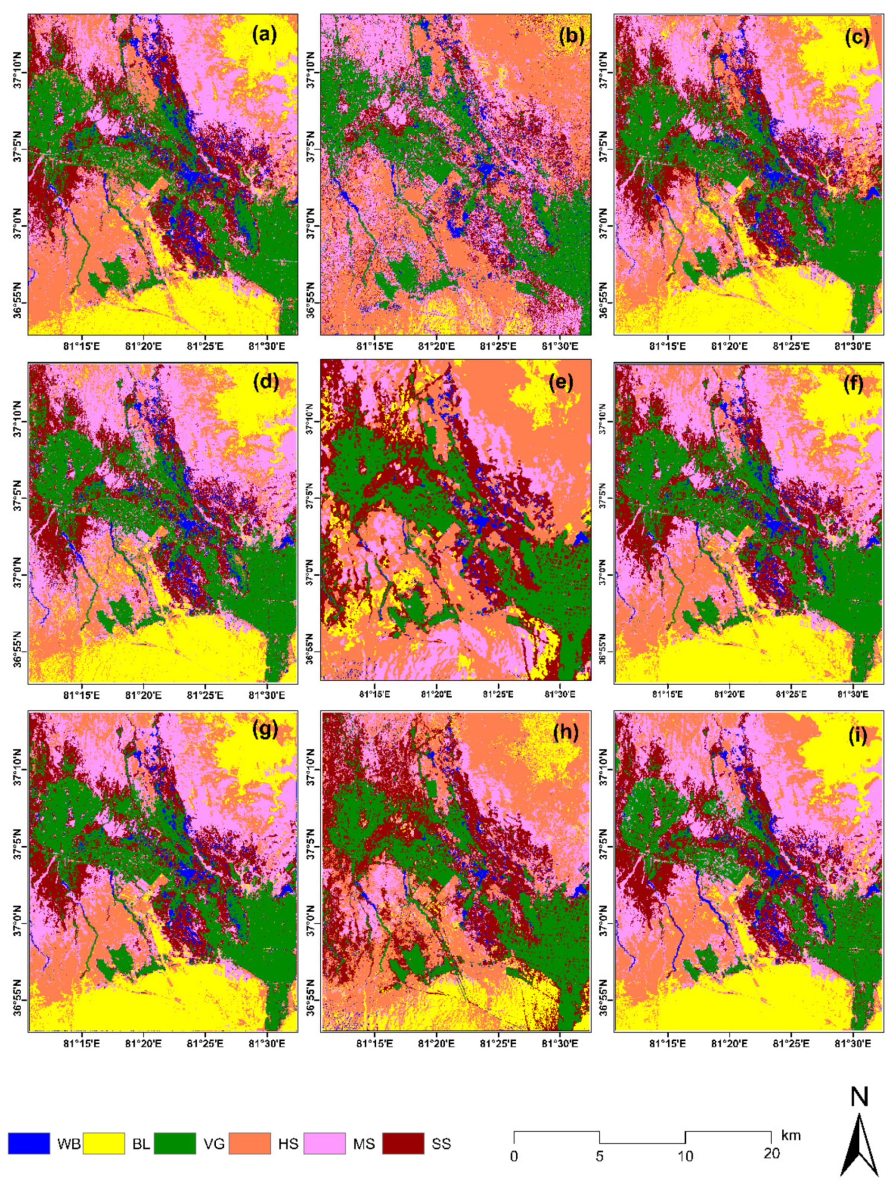
3.2. Classification Results

To extract different degrees of salinized soil, the SVM, RF, and DL methods were used to classify OLI data, PALSAR-2 data, and OLI+PALSAR-2 integrated data. The classification results are displayed in Figure 9.

Figure 9 shows the classification results that most of the study area is bare land (including desert and gravel land), followed by oasis. There were obvious differences in the spatial distributions of the three soil salinization degrees. The salinized soil was distributed at the intersection of the Keriya Oasis and the Taklimakan Desert. The degree of salinization showed a gradual increase trend from oasis to desert. Slightly salinized soil was distributed around the oasis, while strongly and moderately salinized soil was distributed on the periphery of the oasis and the edge of the desert, respectively.

3.3. Classification Accuracy

The results in

Table 5. Validation of the accuracy of the salinized soil information monitoring classification.

Data	SVM		RF		DL
	OA	Kappa	OA	Kappa	OA	Kappa
OLI	84.48%	0.84	87.54%	0.83	89.89 %	0.86
PALSAR-2	77.21%	0.70	79.46%	0.74	80.20%	0.75
OLI+PALSAR-2	87.28%	0.87	90.27%	0.87	91.86%	0.90

Note: OA = Overall accuracy, Kappa = Kappa Coefficient.

indicate that regardless of the classification method, the classification results of the OLI+PALSAR-2 images were relatively positive. In particular, the OLI+PALSAR-2 image classification result of the DL classification was better, having the highest overall accuracy rate of 91.86% and a kappa coefficient of 0.90. The overall accuracy rates of the SVM and RF were 87.28% and 90.27%, and the corresponding kappa coefficients were 0.87 and 0.87, respectively. Compared with the SVM and RF classification, the overall classification accuracy of the DL was increased by 4.53% and 1.59%, respectively.

Figure 10 shows the F1 score, With the growth of Epoch, the F1 scores of all three data tend to increase, the most obvious one is still the OLI+PALSAR-2, followed by OLI data, and the lowest is the PALSAR-2 data.

4. Discussion

4.1. Comparison of Different Classification Methods

The classification results showed that the DL-based method was superior in extracting salinization information. The DL-based CNN algorithm applied convolution computation, which considered the surrounding spatial background for prediction. The SAR images could provide rich spatial and texture details, which were in line with convolution operation and thus could improve the classification accuracy. Therefore, it has been demonstrated that DL can achieve better results in extracting salinization information by using SAR images with clear texture contour information combined with optical images.

Soil salinization, as an environmental problem leading to land degradation and desertification, has been a focus of the attention of foreign researchers. Many researchers used different research methods to extract soil salinity and achieved good results. Nurmemet et al. [23] proposed a WFS-SVM model by using PALSAR-2 data and constructed a salinization detection model, and the result showed that the overall accuracy and Kappa coefficient of the data were 87.57% and 0.85. Feng Juan et al. [110] proposed the SVM-Wishart semi-supervised classification method, which is used to classify the Freeman-Durden decomposition, and the classification accuracy is 88.00%. Machine learning theory has been widely used in remote sensing data, but there are few studies using deep learning to extract soil salinity, especially using radar images combined with deep learning to monitor soil salinization.

In this study, the polarization decomposition theory of radar images and optical images are combined with the method of deep learning to monitor soil salinity information, and slightly better results are achieved. The study shows that there is potential to apply deep learning methods to extract salinization information from radar remote sensing images. However, there are fewer studies on the application of deep learning to radar image monitoring of soil salinization. Although the monitoring results are satisfactory to some extent in this particular arid environment, the generalization of this method in other fields needs further study and evaluation. As a new technical means, it needs to be further improved (future research can try a variety of deep learning models to monitor soil salinity, such as DeepLabv3 [111], PSPNet [112], etc.). We can also try the CRF [113] post-processing method to optimize the classification results and introduce the idea of ensemble learning to integrate the results extracted by various methods to improve the accuracy of classification.

4.2. Polarimetric Decomposition Influence on Classification Results

When extracting soil salinization information by polarimetric decomposition of the PALSAR-2 data, due to the different scattering mechanisms of ground objects, a single coherent matrix and a single target polarimetric decomposition method could not fully exploit the information contained in the radar images. However, the multi-target polarization decomposition method could effectively extract the information of the study area. After polarization decomposition, the structural information of the ground objects was more easily reflected, and the regular texture information was presented better. For instance, the volume scattering component is sensitive to vegetation. The area with vegetation has strong backscattering intensity, while the area with less vegetation has weak backscattering energy. Both single scattering and volume scattering of saline soil were lower than those of vegetation. For slightly and moderately saline land, the vegetation plants were low, and the salinity was different, which made the regions of medium and high scattering entropy strongly random. Strongly salinized soil had the lowest vegetation coverage, and its backscatter value was lower than those of moderately and slightly salinized soil. The scattering value of saline land gradually decreased from slight to strong, and its backscattering value was smaller than that of vegetation. In addition, the characteristic parameters have different sensitivity to the soil information type. The RVI was also beneficial for distinguishing different degrees of salinized soil.

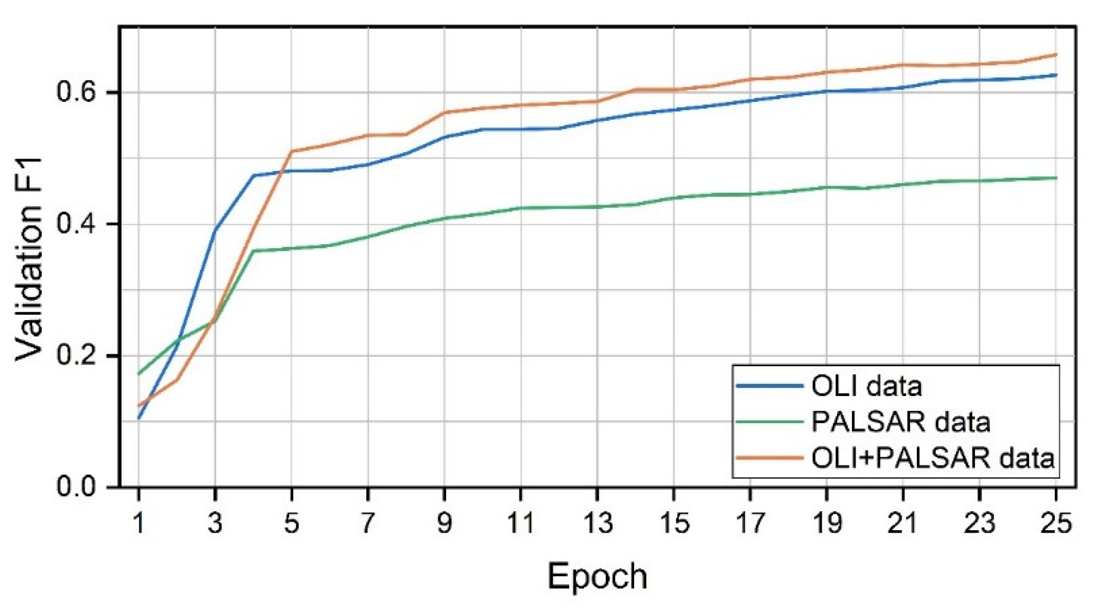
4.3. Data Source Influence on Classification Results

From the comparative analysis results in Figure 9 and Table 5, it can be seen that the overall accuracy of OLI+PALSAR-2 multi-source remote sensing data improved by 1.90%, and the Kappa coefficient improved by 0.04 compared with the OLI optical data when the classification was performed by DL. The overall classification accuracy of OLI+PALSAR-2 data improved by 2.73% and 2.8% compared with OLI data when classified by RF and SVM, and the Kappa coefficients improved by 0.04 and 0.03, respectively. The overall distribution of salinized soils was well reflected from the DL classification. From east to west, the land cover types shift from vegetation to slightly salinized soil, moderately salinized soil, and strongly salinized soil. This is partly due to the high spatial resolution and apparent polarized backscattering characteristics of the SAR data, and the improved spectral and spatial quality of the band-synthesized images, which enhance the discrimination of different salinized soils. This study aims to make full use of the advantages of optical remote sensing data and radar remote sensing data. Although the spatial resolution of optical data was not high and the texture contour information was not obvious, it provided abundant spectral information in the visible-light range. The NDVI and SI could effectively extract soil salinization and vegetation information. Moreover, although radar data had high speckle noise, it had clear contour texture information and high spatial resolution. These two data could complement each other’s shortcomings and could better extract salt information.

4.4. Distribution Characteristics of Salinization in Study Area

The results demonstrated that the degree, scope, and spatial distribution of soil salinization were different in different regions of the research area. The main reason was that the study site was affected by the dry and rainless climate conditions and had a strong dependence on water resources. Tarim Basin is formed by three mountains sandwiched by two basins and is located in a closed inland environment, making it impossible for soil salt to run off to the surrounding areas [43]. In addition, the elevation in the north of the study area was lower than that in the south, which increased the depth of groundwater. Furthermore, high-temperature conditions induced strong transpiration, which made soluble salts accumulate to the soil surface with soil moisture under capillary action, leading to the increase in the soil salt content.

5. Conclusions

In this study, the PALSAR-2 and Landsat-8-OLI (OLI) images are combined with a deep learning (DL)-based method and used to monitor the soil salinization in the Keriya oasis to effectively promote the stability of the ecological environment and the sustainable development of agriculture in the research area.

(1)

A variety of target polarization decomposition methods, including the Pauli, Freeman, Freeman_Durden, Cloude, Yamaguchi, VanZyl, Sinclair, and H/A/Alpha methods, are used to polarize the PALSAR-2 data. Additionally, the eight best feature components, namely $T_{33}$, $C_{33}$, Freeman Durden_vol_g, Pauli_b, Pauli_r, Sinclair_g, VanZyl_vol_g, and RVI, are selected by the random forest (RF) method to extract the information on soil salinization.

(2)

The OLI data are used to extract the normalized vegetation index (NDVI) and salinity index (SI), which are then combined with the optimal feature subsets of the PALSAR-2 image to form an integrated image to extract salinization information.

(3)

Classification methods, such as a support vector machine (SVM), RF, and DL, are used to extract salinization information from different data types, including the OLI, PALSAR-2, and OLI+PALSAR-2 data. The results show that the OLI+PALSAR-2 image classification result of the DL classification was relatively good, having the highest overall accuracy rate of 91.86% and a kappa coefficient of 0.90.

References

1. El Harti, A.; Lhissou, R.; Chokmani, K.; Ouzemou, J.; Hassouna, M.; Bachaoui, E.M.; El Ghmari, A. Spatiotemporal Monitoring of Soil Salinization in Irrigated Tadla Plain (Morocco) Using Satellite Spectral Indices. Int. J. Appl. Earth Obs. Geoinf. 2016, 50, 64–73. [Google Scholar] [CrossRef]
2. Akça, E.; Aydin, M.; Kapur, S.; Kume, T.; Nagano, T.; Watanabe, T.; Çilek, A.; Zorlu, K. Long-term monitoring of soil salinity in a semi-arid environment of Turkey. Catena 2020, 193, 104614. [Google Scholar] [CrossRef]
3. Naimi, S.; Ayoubi, S.; Zeraatpisheh, M.; Dematte, J.A.M. Ground Observations and Environmental Covariates Integration for Mapping of Soil Salinity: A Machine Learning-Based Approach. Remote Sens. 2021, 13, 4825. [Google Scholar] [CrossRef]
4. Yu, P.Y. Effects of Potassium Ion on Physiologicalproperty of Malus Zumi Seedling under Salt. Master’s Thesis, Tianjin Agricultural University, Tianjin, China, 2014. (In Chinese). [Google Scholar]
5. Bell, D.; Menges, C.; Ahmad, W.; van Zyl, J.J. The application of dielectric retrieval algorithms for mapping soil salinity in a tropical coastal environment using airborne polarimetric SAR. Remote Sens. Environ. 2001, 75, 375–384. [Google Scholar] [CrossRef]
6. Li, J.G.; Pu, L.J.; Zhu, M.; Zhang, R.S. The present situation and hot issues in the salt-affected soil research. Acta Geogr. Sin. 2012, 67, 1233–1245. (In Chinese) [Google Scholar]
7. Singh, A.; Meena, G.K.; Kumar, S.; Gaurav, K. Evaluation of the Penetration Depth of L-and S-Band (NISAR mission) Microwave SAR Signals into Ground. In Proceedings of the 2019 URSI Asia-Pacific Radio Science Conference (AP-RASC), New Delhi, India, 9–15 March 2019; p. 1. [Google Scholar]
8. Jakob Van Zyl, Y.K. Synthetic Aperture Radar Polarimetry; John Wiley & Sons: Hoboken, NJ, USA, 2011; Volume 2. [Google Scholar]
9. Fan, Z.L.; Xu, Q.Q.; Li, H.P.; Zhang, P.; Zhou, S.B.; Lu, L. Rational groundwater exploitation and utilization, an important approach of improving Salinized Farmland in Xinjiang. Arid Zone Res. 2011, 28, 737–743. (In Chinese) [Google Scholar]
10. Muhetaer, N.; Nurmemet, I.; Abulaiti, A.; Xiao, S.; Zhao, J. A Quantifying Approach to Soil Salinity Based on a Radar Feature Space Model Using ALOS PALSAR-2 Data. Remote Sens. 2022, 14, 363. [Google Scholar] [CrossRef]
11. Allbed, A.; Kumar, L. Soil salinity mapping and monitoring in arid and semi-arid regions using remote sensing technology: A review. Adv. Remote Sens. 2013, 2, 373–385. [Google Scholar] [CrossRef] [Green Version]
12. Andrade, G.R.P.; Furquim, S.A.C.; do Nascimento, T.T.V.; Brito, A.C.; Camargo, G.R.; de Souza, G.C. Transformation of clay minerals in salt-affected soils, Pantanal wetland, Brazil. Geoderma 2020, 371, 114380. [Google Scholar] [CrossRef]
13. Qi, Z.; Yeh, A.G.O.; Li, X.; Lin, Z. A novel algorithm for land use and land cover classification using RADARSAT–2 polarimetric SAR data. Remote Sens. Environ. 2012, 118, 21–39. [Google Scholar] [CrossRef]
14. Bindlish, R.; Barros, A.P. Parameterization of vegetation backscatter in radar-based, soil moisture estimation. Remote Sens. Environ. 2001, 76, 130–137. [Google Scholar] [CrossRef]
15. Maghsoudi, Y.; Collins, M.J.; Leckie, D.G. Radarsat–2 polarimetric SAR data for boreal forest classification using SVM and a wrapper feature selector. IEEE J. Sel. Top. Appl. Earth Obs. Remote Sens. 2013, 6, 1531–1538. [Google Scholar] [CrossRef]
16. Del Frate, F.; Ferrazzoli, P.; Schiavon, G. Retrieving soil moisture and agricultural variables by microwave radiometry using neural networks. Remote Sens. Environ. 2003, 84, 174–183. [Google Scholar] [CrossRef]
17. Serbin, G.; Or, D. Ground-penetrating radar measurement of soil water content dynamics using a suspended horn antenna. IEEE Trans. Geosci. Remote Sens. 2004, 42, 1695–1705. [Google Scholar] [CrossRef]
18. Rhoades, J.D.; Chanduvi, F. Soil Salinity Assessment: Methods and Interpretation of Electrical Conductivity Measurements; Food & Agriculture Organazition: Rome, Italy, 1999. [Google Scholar]
19. Zhu, Z.; Woodcock, C.E.; Rogan, J.; Kellndorfer, J. Assessment of spectral, polarimetric, temporal, and spatial dimensions for urban and peri-urban land cover classification using Landsat and SAR data. Remote Sens. Environ. 2012, 117, 72–82. [Google Scholar] [CrossRef]
20. Negra, T.; Ilyas, N.; Wang, Y.H.; Mukaddas, A. Soil Salinization Classification in Arid Area Based on H/A/α Decomposition Fully Polarized SAR Data. Jiangsu Agr. Sci. 2019, 47, 273–279. (In Chinese) [Google Scholar]
21. Wang, Y.Y. Classification of Polarimetric SAR Images Based on Multilaver Network Model. Ph.D. Thesis, Wuhan University, Wuhan, China, 2015. (In Chinese). [Google Scholar]
22. Qu, Y.C. Polarimetric Radarsat–2 Image Classification Based on Target Decomposition Theorems in Polarimetry. Master’s Thesis, Nanjing University, Nanjing, China, 2016. (In Chinese). [Google Scholar]
23. Nurmemet, I.; Sagan, V.; Ding, J.L.; Halik, U.; Abliz, A.; Yakup, Z. A WFS-SVM model for soil salinity mapping in keriya oasis, northwestern china using polarimetric decomposition and fully PolSAR data. Remote Sens. 2018, 10, 598. [Google Scholar] [CrossRef] [Green Version]
24. Weilei, D. The Research on Target Recognition Methods Based on Polarization Radar. Master’s Thesis, Harbin Engineering University, Harbin, China, 2013. [Google Scholar]
25. Luo, C.; Feng, X.; Liu, C.; Zhang, Y.; Nilot, E.; Zhang, M.; Dong, Z.; Zhou, H. Full-polarimetric GPR for detecting ice fractures. In Proceedings of the 2018 17th International Conference on Ground Penetrating Radar (GPR), Rapperswil, Switzerland, 18–21 June 2018; pp. 1–4. [Google Scholar]
26. Isak, G.; Nurmemet, I.; Duan, S.S. The Extraction of Saline Soil Information in Typical Oasis of Arid Area Using Fully Polarimetric Radarsat-2 data. China Rural. Water Hydropower 2018, 12, 13–19. [Google Scholar]
27. Xiao, Y. Research on Object-Oriented Classification. Master’s Thesis, Jilin University, Changchun, China, 2017. (In Chinese). [Google Scholar]
28. Aldabaa, A.A.A.; Weindorf, D.C.; Chakraborty, S.; Sharma, A.; Li, B. Combination of proximal and remote sensing methodsfor rapid soil salinity quantification. Geoderma 2015, 239-240, 34–46. [Google Scholar] [CrossRef] [Green Version]
29. XIE, X.Q.; Yang, J.Z.; Deng, S.W. Identifying flue-cured tobacco in a typical cultivated area of Yuxi based on Sentinel-1 time series images. J. Agric. Resour. Environ. 2022, 41, 21–39. [Google Scholar]
30. Taghadosi, M.M.; Hasanlou, M.; Eftekhari, K. Soil salinity mapping using dual-polarized SAR Sentinel-1 imagery. Int. J. Remote Sens. 2018, 40, 237–252. [Google Scholar] [CrossRef]
31. Tan, M.; Pang, R.; Le, Q.V. Efficientdet: Scalable and Efficient Object Detection. Available online: https://openaccess.thecvf.com/content_CVPR_2020/papers/Tan_EfficientDet_Scalable_and_Efficient_Object_Detection_CVPR_2020_paper.pdf (accessed on 4 January 2022).
32. Yan, X.; Cui, B.; Xu, Y.; Shi, P.; Wang, Z. A method of information protection for collaborative deep learning under gan model attack. IEEE/ACM Trans. Comput. Biol. Bioinform. 2019, 18, 871–881. [Google Scholar]
33. Otter, D.W.; Medina, J.R.; Kalita, J.K. A survey of the usages of deep learning for natural language processing. IEEE Trans. Neural Netw. Learn. Syst. 2021, 32, 604–624. [Google Scholar] [CrossRef] [Green Version]
34. Gao, J.; Deng, B.; Qin, Y.; Wang, H.; Li, X. Enhanced radar imaging using a complex-valued convolutional neural network. IEEE Geosci. Remote Sens. Lett. 2019, 16, 35–39. [Google Scholar] [CrossRef] [Green Version]
35. Zhou, Y.; Wang, H.; Xu, F.; Jin, Y. Polarimetric SAR image classification using deep convolutional neural networks. IEEE Geosci. Remote Sens. Lett. 2017, 13, 1935–1939. [Google Scholar] [CrossRef]
36. Jiang, T.; Cui, Z.; Zhou, Z.; Cao, Z. Data Augmentation with Gabor Filter in Deep Convolutional Neural Networks for Sar Target Recognition. In Proceedings of the IGARSS 2018—2018 IEEE International Geoscience and Remote Sensing Symposium, Valencia, Spain, 22–27 July 2018; pp. 689–692. [Google Scholar] [CrossRef]
37. Zhang, C.; Sargent, I.; Pan, X.; Li, H.; Gardiner, A.; Hare, J.; Atkinson, P.M. An object-based convolutional neural network (OCNN) for urban land use classification. Remote Sens. Environ. 2018, 216, 57–70. [Google Scholar] [CrossRef] [Green Version]
38. Ndikumana, E.; Minh, D.H.T.; Baghdadi, N.; Courault, D.; Hossard, L. Applying deep learning for agricultural classification using multitemporal SAR Sentinel-1 for Camargue, France. In Image and Signal Processing for Remote Sensing Xxiv; Bruzzone, L., Bovolu, F., Eds.; Spie-Int Soc Optical Engineering: Bellingham, WA, USA, 2018. [Google Scholar]
39. Hou, B.; Kou, H.; Jiao, L. Classification of polarimetric sar images using multilayer autoencoders and superpixels. IEEE J. Sel. Top. Appl. Earth Obs. Remote Sens. 2016, 9, 3072–3081. [Google Scholar] [CrossRef]
40. Zhu, L.K.; Ma, X.S.; Wu, P.H.; Xu, J.G. Multiple classifiers based semi-supervised polarimetric SAR image classification method. Sensors 2021, 21, 3006. [Google Scholar] [CrossRef] [PubMed]
41. Ghulam, A.; Qin, Q.; Zhu, L.; Abdrahman, P. Satellite remote sensing of groundwater: Quantitative modelling and uncertainty reduction using 6s atmospheric simulations. Int. J. Remote Sens. 2004, 25, 5509–5524. [Google Scholar] [CrossRef]
42. Hao, X.; Chen, Y.; Li, W.; Guo, B.; Zhao, R. Hydraulic lift in Populus euphratica Oliv from the desert riparian vegetation of the Tarim River Basin. J. Arid Environ. 2010, 74, 905–911. [Google Scholar] [CrossRef]
43. Yang, X. The oases along the Keriya River in the Taklamakan Desert, China, and their evolution since the end of the last glaciation. Environ. Geol. 2001, 41, 314–320. [Google Scholar]
44. Dong, X.G.; Deng, M. Groundwater Resources in Xinjiang; Xinjiang Science and Technology Publishing House: Urumqi, China, 2009; pp. 8–9. (In Chinese) [Google Scholar]
45. Zaytungul, Y.; Mamat, S.; Abdusalam, A.; Zhang, D. Soil salinity inversion in Yutian Oasis based on PALSAR radar data. Res. Sci. 2018, 40, 2110–2117. [Google Scholar]
46. Rosenqvist, A.; Shimada, M.; Suzuki, S.; Ohgushi, F.; Tadono, T.; Watanabe, M.; Tsuzuku, K.; Watanabe, T.; Kamijo, S.; Aoki, E. Operational performance of the ALOS global systematic acquisition strategy and observation plans for ALOS–2 PALSAR–2. Remote Sens. Environ. 2014, 155, 3–12. [Google Scholar] [CrossRef]
47. Natsuaki, R.; Nagai, H.; Motohka, T.; Ohki, M.; Watanabe, M.; Thapa, R.B.; Tadono, T.; Shimada, M.; Suzuki, S. SAR interferometry using ALOS–2 PALSAR–2 data for the Mw 7. 8 Gorkha, Nepal earthquake. Earth Planets Space 2016, 68, 15. [Google Scholar] [CrossRef] [Green Version]
48. Suzuki, S.; Kankaku, Y.; Osawa, Y. Development Status of PALSAR–2 onboard ALOS–2. Technol. Rep. Ieice Sane 2011, 113, 1–4. [Google Scholar]
49. Arikawa, Y.; Saruwatari, H.; Hatooka, Y.; Suzuki, S. ALOS–2 launch and early orbit operation result. Int. Geosci. Remote Sens. Symp. 2014, 2, 3406–3409. [Google Scholar]
50. Lopes, A.; Touzi, R.; Nezry, E. Adaptive speckle filters and scene heterogeneity. IEEE Trans. Geosci. Remote Sens. 1990, 28, 992–1000. [Google Scholar] [CrossRef]
51. Holecz, F.; Meier, E.; Piesbergen, J.; Nisch, D.; Moreira, J. Rigorous derivation of backscattering coefficient. IEEE Geosc. Remote Sens. Soc. Newsl. 1994, 92, 6–14. [Google Scholar]
52. Sarmap, S.A. Synthetic Aperture Radar and SARscape: SAR Guidebook; Purasca: Caslano, Switzerland, 2009. [Google Scholar]
53. Ulaby, F.T.; Dobson, M.C. Handbook of Radar Scattering Statistics for Terrain; Artech House: Norwood, MA, USA, 1989. [Google Scholar]
54. Mashimbye, Z.E.; Cho, M.A.; Nell, J.P.; De Clercq, W.P.; Van Niekerk, A.; Turner, D.P. Model-Based Integrated Methods for Quantitative Estimation of Soil Salinity from Hyperspectral Remote Sensing Data: A Case Study of Selected South African Soils. Pedosphere 2012, 22, 640–649. [Google Scholar] [CrossRef]
55. Zhang, J.; Zhang, Z.; Chen, J.; Chen, H.; Jin, J.; Han, J.; Wang, X.; Song, Z.; Wei, G. Estimating soil salinity with different fractional vegetation cover using remote sensing. Land Degrad. Develop. 2020, 32, 597–612. [Google Scholar] [CrossRef]
56. Huynen, J.R. Phenomenological Theory of Radar Targets. Ph.D. Thesis, Technical University, Delft, The Netherlands, 1970. [Google Scholar]
57. An, W.T.; Cui, Y.; Yang, J. Three-Component Model-Based Decomposition for Polarimetric SAR Data. IEEE Trans. Geosci. Remote Sens. 2010, 48, 2732–2739. [Google Scholar]
58. Cloude, S.R. Groupe theory and polarization algebra. Optic 1986, 75, 26–36. [Google Scholar]
59. Huang, X.D. The Inconsistency of Polarimetric Sar Model-Based Target Decomposition. Master’s Thesis, China University of Geoscience, Wuhan, China, 2013. [Google Scholar]
60. He, M.; Li, Y.Z.; Wang, X.S.; Xiao, S.P.; Li, Z.J. A polarimetric calibration algorithm based on pauli-basis decomposition. J. Astronaut. 2011, 32, 2589–2595. [Google Scholar]
61. Lee, J.S.; Pottier, E. Polarimetric Radar Imaging: From Basics to Applications; CRC Press: New York, NY, USA, 2009. [Google Scholar]
62. Cloude, S.R. Target decomposition theorems in radar scattering. Electron. Lett. 1985, 21, 22–24. [Google Scholar] [CrossRef]
63. Freeman, A. Fitting a two-component scattering model to polarimetric SAR data from forests. IEEE Trans. Geosci. Remote Sens. 2007, 45, 2583–2592. [Google Scholar] [CrossRef]
64. Cloude, S.R.; Pottier, E. An entropy based classification scheme for land applications of polarimetric SAR. IEEE Trans. Geosci. Remote Sens. 1997, 35, 68–78. [Google Scholar] [CrossRef]
65. Freeman, A.; Durden, S.L. A three-component scattering model for polarimetric SAR data. IEEE Trans. Geosci. Remote Sens. 1998, 36, 963–973. [Google Scholar] [CrossRef] [Green Version]
66. Zhang, W.; Yin, F.; Chai, J.; Bai, X. The Effect of Send/Receive Dual Channel Parameters on Polarization Parameters Measurement. Chin. J. Electron. 2017, 26, 336–344. [Google Scholar] [CrossRef]
67. Van Zyl, J.J. Application of Cloude’s target decomposition theorem to polarimetric imaging radar data. In Radar Polarimetry; International Society for Optics and Photonics: Bellingham, WA, USA, 1993; pp. 184–191. [Google Scholar]
68. Yamaguchi, Y.; Moriyama, T.; Ishido, M.; Yamada, H. Four-component scattering model for polarimetric SAR image decomposition. IEEE Trans. Geosci. Remote Sens. 2005, 43, 1699–1706. [Google Scholar] [CrossRef]
69. Ersahin, K.; Cumming, I.G.; Ward, R.K. Segmentation and Classification of Polarimetric SAR Data Using Spectral Graph Partitioning. IEEE Trans. Geosci. Remote Sens. 2010, 48, 164–174. [Google Scholar] [CrossRef] [Green Version]
70. Abuelgasim, A.; Ammad, R. Mapping soil salinity in arid and semi-arid regions using Landsat-8 OLI satellite data. Remote Sens. Appl. Soc. Environ. 2019, 13, 415–425. [Google Scholar] [CrossRef]
71. Xie, Q.; Meng, Q.; Zhang, L.; Wang, C.; Sun, Y.; Sun, Z. A Soil Moisture Retrieval Method Based on Typical Polarization Decomposition Techniques for a Maize Field from Full-Polarization Radarsat-2 Data. Remote Sens. 2017, 9, 168. [Google Scholar] [CrossRef] [Green Version]
72. He, C.; Xia, G.; Sun, H. SAR images classification method based on Dempster-Shafer theory and kernel estimate. J. Syst. Eng. Electron. 2007, 18, 210–216. [Google Scholar]
73. Defries, R.S.; Townshend, J.R.G. NDVI-derived land cover classifications at a global scale. Int. J. Remote Sens. 1994, 15, 3567–3586. [Google Scholar] [CrossRef]
74. Wang, F.; Chen, X.; Luo, G.; Ding, J.; Chen, X. Detecting soil salinity with arid fraction integrated index and salinity index in feature space using Landsat TM imagery. J. Arid Land 2013, 5, 340–353. [Google Scholar] [CrossRef] [Green Version]
75. Xie, Q.; Lai, K.; Wang, J.; Lopez-Sanchez, J.M.; Shang, J.; Liao, C.; Zhu, J.; Fu, H.; Peng, X. Crop Monitoring and Classification Using Polarimetric RADARSAT-2 Time-Series Data Across Growing Season: A Case Study in Southwestern Ontario, Canada. Remote Sens. 2021, 13, 1394. [Google Scholar] [CrossRef]
76. Pottier, E.; Ferro-Famil, L. PolSARPro V5.0: An ESA educational toolbox used for self-education in the field of POLSAR and POL-INSAR data analysis. In Proceedings of the 2012 IEEE International Geoscience and Remote Sensing Symposium, Munich, Germany, 22–27 July 2012; pp. 7377–7380. [Google Scholar]
77. Breiman, L. Bagging predictors. Mach. Learn. 1996, 24, 123–140. [Google Scholar] [CrossRef] [Green Version]
78. Genuer, R.; Poggi, J.M. Variable selection using randomforest. Pattern Recognit. Lett. 2010, 31, 2225–2236. [Google Scholar] [CrossRef] [Green Version]
79. Han, P.; Sun, D.D. Classification of Polarimetric SAR image with feature selection and deep learning. J. Signal Process. 2019, 35, 972–978. [Google Scholar]
80. Vapnik, V.N. The Nature of Statistical Learning Theory; Springer: Berlin, Germany, 1995. [Google Scholar]
81. Chang, C.C.; Lin, C.J. LIBSVM: A library for support vector machines. ACM Trans. Intell. Syst. Technol. 2011, 2, 1–27. [Google Scholar] [CrossRef]
82. Keerthi, S.S.; Lin, C.J. Asymptotic behaviors of support vector machines with Gaussian kernel. Neural Comput. 2003, 15, 1667–1689. [Google Scholar] [CrossRef]
83. Breiman, L. Random forests. Mach. Learn. 2001, 45, 5–32. [Google Scholar] [CrossRef] [Green Version]
84. Ho, T. The random subspace method for constructing decision forests. IEEE Trans. Pattern Anal. 1998, 20, 832–844. [Google Scholar]
85. Ibrahim, M. Reducing correlation of random forest based learning-to-rank algorithms using subsample size. Comput. Intell. 2019, 35, 774–798. [Google Scholar] [CrossRef]
86. Friedman, J.; Hastie, T.; Tibshirani, R. The Elements of Statistical Learning; Springer Series in Statistics; Springer: New York, NY, USA, 2001. [Google Scholar]
87. Liu, M.; Lang, R.L.; Cao, Y.B. Number of trees in random forest. Comput. Eng. Appl. 2015, 51, 126–131. (In Chinese) [Google Scholar]
88. Zhang, L.P.; Zhang, L.F.; Du, B. Deep learning for remote sending data: A technical tutorial on the state of the art. IEEE Geosci. Remote Sens. Mag. 2016, 4, 22–40. (In Chinese) [Google Scholar] [CrossRef]
89. Wang, J.; Zheng, T.; Lei, P.; Wei, S.M. Study on deep learning in radar. J. Radars 2018, 7, 395–411. (In Chinese) [Google Scholar]
90. Pan, Z.X.; An, Q.Z.; Zhang, B.C. Progress of deep learning-based target recognition in radar images. Sci. Sin. Inform. 2019, 49, 1626–1639. (In Chinese) [Google Scholar]
91. Tao, C.S. Reasearch of Polarimetric SAR Detection and Classification Based on Features in Rotation Domain and Deep CNN. Master’s Thesis, National University of Defense Technology, Changsha, China, 2017. (In Chinese). [Google Scholar]
92. Hua, W.Q. Study on Polarimetric SAR Images Classification with Small Samples. Master’s Thesis, Xidian University, Xi’an, China, 2018. (In Chinese). [Google Scholar]
93. Zhu, X.X.; Tuia, D.; Mou, L.C.; Xia, G.S.; Zhang, L.P.; Xu, F.; Fraundorfer, F. Deep learning in remote sensing: A comperehensive review and list of resources. IEEE Geosc. Remote Sens. Mag. 2017, 5, 8–36. [Google Scholar] [CrossRef] [Green Version]
94. Deng, S.P.; Sun, S. Comparisions of polarimetric SAR image classifiers based on deep learning. Sci. Survey. Map. 2021, 46, 120–127. (In Chinese) [Google Scholar]
95. Zhai, Y.K.; Ma, H.; Cao, H.; Deng, W.B.; Liu, J.; Zhang, Z.Y.; Guan, H.X.; Zhi, Y.H.; Wang, J.X.; Zhou, J.H. MF-SarNet: Effective CNN with data augmentation for SAR automatic target recognition. J. Eng. 2019, 2019, 5813–5818. [Google Scholar] [CrossRef]
96. Li, Q.; Cai, W.; Wang, X.; Zhou, Y.; Feng, D.D.; Chen, M. Medical image classification with convolutional neural network. In Proceedings of the 2014 13th International Conference on Control Automation Robotics & Vision (ICARCV), Singapore, 10–12 December 2014; pp. 844–848. [Google Scholar]
97. Li, G.Q.; Bai, Y.Q.; Yang, X.; Chen, Z.C.; Yu, H.K. Automatic deep learning land cover classification methods of high-resolution remotely sensed images. J. Geo-Inform. Sci. 2021, 23, 1690–1704. (In Chinese) [Google Scholar]
98. Long, J.; Shelhamer, E.; Darrell, T. Fully convolutional networks for semantic segmentation. In Proceedings of the 2015 IEEE Conference on Computer Vision and Pattern Recognition (CVPR), Boston, MA, USA, 7–12 June 2015; pp. 3431–3440. [Google Scholar]
99. Ronneberger, O.; Fischer, P.; Brox, T. U-Net: Convolutional networks for biomedical image segmentation. In Proceedings of the International Conference on Medical Image Computing and Computer-Assisted Intervention, Munich, Germany, 5–9 October 2015; pp. 234–241. [Google Scholar]
100. Badrinarayanan, V.; Kendall, A.; Cipolla, R. SegNet: A deep convolutional encoder-decoder architecture for image segmentation. IEEE Trans. Pattern Anal. 2017, 39, 2481–2495. [Google Scholar] [CrossRef] [PubMed]
101. He, K.M.; Zhang, X.Y.; Ren, S.Q.; Sun, J. Deep residual learning for image recognition. In Proceedings of the 2016 IEEE Conference on Computer Vision and Pattern Recognition (CVPR), Las Vegas, NV, USA, 27–30 June 2016; pp. 770–778. [Google Scholar]
102. Chen, L.C.; Papandreou, G.; Kokkinos, I.; Murphy, K.; Yuille, A.L. DeepLab: Semantic image segmentation with deep convolutional nets, atrous convolution, and fully connected CRFs. IEEE Trans. Pattern Anal. 2018, 40, 834–848. [Google Scholar] [CrossRef] [Green Version]
103. Chen, L.; Zhu, Y.; Papandreou, G.; Schroff, F.; Adam, H. Encoder-Decoder with atrous separable convolution for semantic image segmentation. In Proceedings of the European conference on computer vision (ECCV), Munich, Germany, 8–14 September 2018; pp. 33–851. [Google Scholar]
104. Xu, H.M. Method Research of High Resolution Remote Sensing Imagery Classification Based on U-Net Model of Deep Learning. Master’s Thesis, Southwest Jiaotong University, Chengdu, China, 2018. (In Chinese). [Google Scholar]
105. Ibtehaz, N.; Rahman, M.S. MultiResUNet: Rethinking the U-Net architecture for multimodal biomedical image segmentation. Neural Netw. 2020, 121, 74–87. [Google Scholar] [CrossRef]
106. Pontius, R.G.; Millones, M. Death to Kappa: Birth of quantity disagreement and allocation disagreement for accuracy assessment. Int. J. Remote Sens. 2011, 32, 4407–4429. [Google Scholar] [CrossRef]
107. Congalton, R.G. A review of assessing the accuracy of classifications of remotely sensed data. Remote Sens. Environ. 1991, 37, 35–46. [Google Scholar] [CrossRef]
108. Hand, D.J.; Christen, P.; Kirielle, N. F*: An interpretable transformation of the F-measure. Mach. Learn. 2021, 110, 451–456. [Google Scholar] [CrossRef] [PubMed]
109. Erenel, Z.; Altincay, H. Improving the precision-recall trade-off in undersampling-based binary text categorization using unanimity rule. Neural Comput. Appl. 2013, 22, S83–S100. [Google Scholar] [CrossRef]
110. Feng, J.; Ding, J.L.; Wei, W.Y. Soil salinization monitoring based on Radar data. Remote Sens. Land Resour. 2019, 31, 195–203. [Google Scholar]
111. Wang, D.; Wan, J.; Liu, S.; Chen, Y.; Yasir, M.; Xu, M.; Ren, P. BO-DRNet: An Improved Deep Learning Model for Oil Spill Detection by Polarimetric Features from SAR Images. Remote Sens. 2022, 14, 264. [Google Scholar] [CrossRef]
112. Wu, F.; Wang, C.; Zhang, H.; Li, J.; Li, L.; Chen, W.; Zhang, B. Built-up area mapping in China from GF-3 SAR imagery based on the framework of deep learning. Remote Sens. Environ. 2021, 262, 112515. [Google Scholar] [CrossRef]
113. Shi, C.; Jiang, Q.; Duan, F.; Shi, P. GF-2 Landuse classification based on UNET+CRF. Glob. Geol. 2021, 40, 146–153. [Google Scholar]
Figure 1. Location map of the study area showing the overview map of China and the Xinjiang (A,B); (C) Topographic map of the study area; (D) Location map of the study area in Landsat-8-OLI image; (E) the subset image covering the study area in Pauli decomposition with standard color-coding (Red: |HH − VV|, Green: |HV|, Blue: |HH + VV|).
Sustainability 14 02666 g001
Figure 2. Preprocessing flowchart of PALSAR-2 data.
Sustainability 14 02666 g002
Figure 3. Different degrees of salinized soil and land cover types of Keriya Oasis of the study area. (a) Strongly salinized soil; (b) Strongly salinized soil; (c) Desert; (d) Moderately salinized soil; (e) Moderately salinized soil; (f) Water body; (g) Slightly salinized soil; (h) Slightly salinized soil; (i) Vegetation.
Sustainability 14 02666 g003
Figure 4. Overall workflow of the study.
Sustainability 14 02666 g004
Figure 5. Schematic diagram of a typical CNN network structure.
Sustainability 14 02666 g005
Figure 6. RGB composition images of different polarimetric decompositions and SAR discriminators including Pauli decomposition (a); Cloude decomposition (b); Freeman decomposition (c); H/A/Alpha decomposition (d); Freeman durden decomposition (e); Sinclair decomposition (f); Vanzyl decomposition (g); Yamaguchi decomposition (h); RVI (i).
Sustainability 14 02666 g006
Figure 7. Ranking of importance of features.
Sustainability 14 02666 g007
Figure 8. PolSAR data optimal features subset including: pauli_b (a); pauli_r (b); Freemen durden_vol_g (c); Sinclair_g (d); Vanzyl_g (e).
Sustainability 14 02666 g008
Figure 9. Comparison of different data sources and different classification results. (a) OLI data SVM classification; (b) PALSAR-2 data SVM classification; (c) OLI+PALSAR-2 data SVM classification; (d) OLI data RF classification; (e) PALSAR-2 data RF classification; (f) OLI+PALSAR-22 data RF classification; (g) OLI data DL classification; (h) PALSAR-2 data DL classification; (i) OLI+PALSAR-2 DL classification. WB, BL, VG, HS, MS, and SS represent the water body, barren land, vegetation, highly salinized soil, moderately salinized soil, and slightly salinized soil, respectively.
Sustainability 14 02666 g009
Figure 10. Validation F1 score (The F1 score is the summed average of the user accuracy and the producer accuracy).
Sustainability 14 02666 g010