
Commuter Bus Operation Rules under Two Traffic Scenarios and Two Weather Conditions: Naturalistic Driving Study on Vehicle Speed and Clearance

 ,
, 
Abstract
:1. Introduction
2. Methods and Materials
2.1. Participants
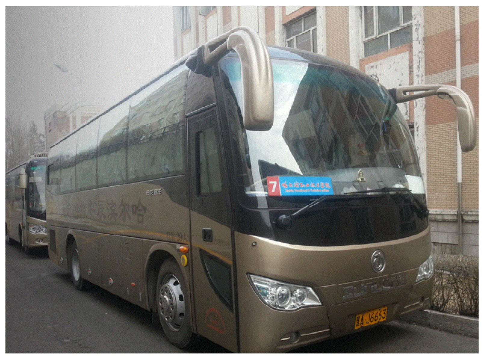
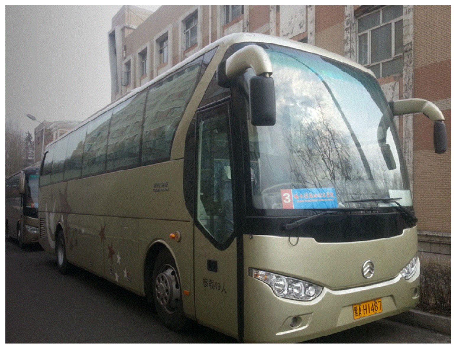
2.2. Vehicles and Buses Seats
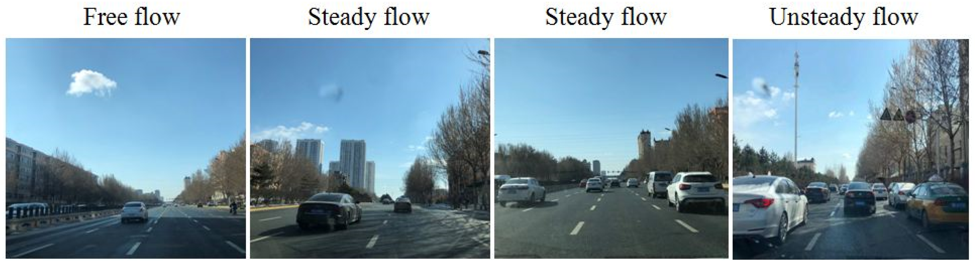
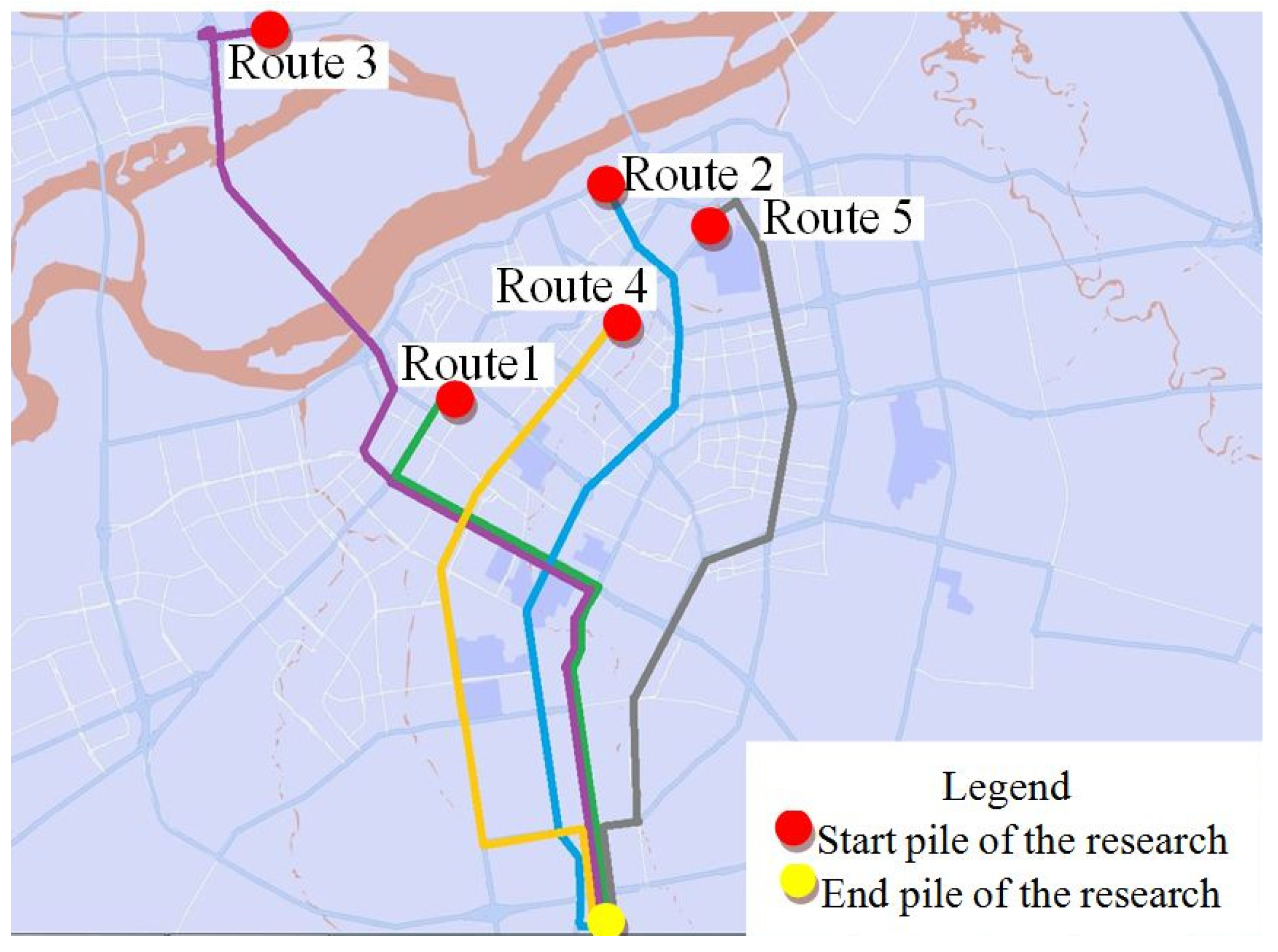
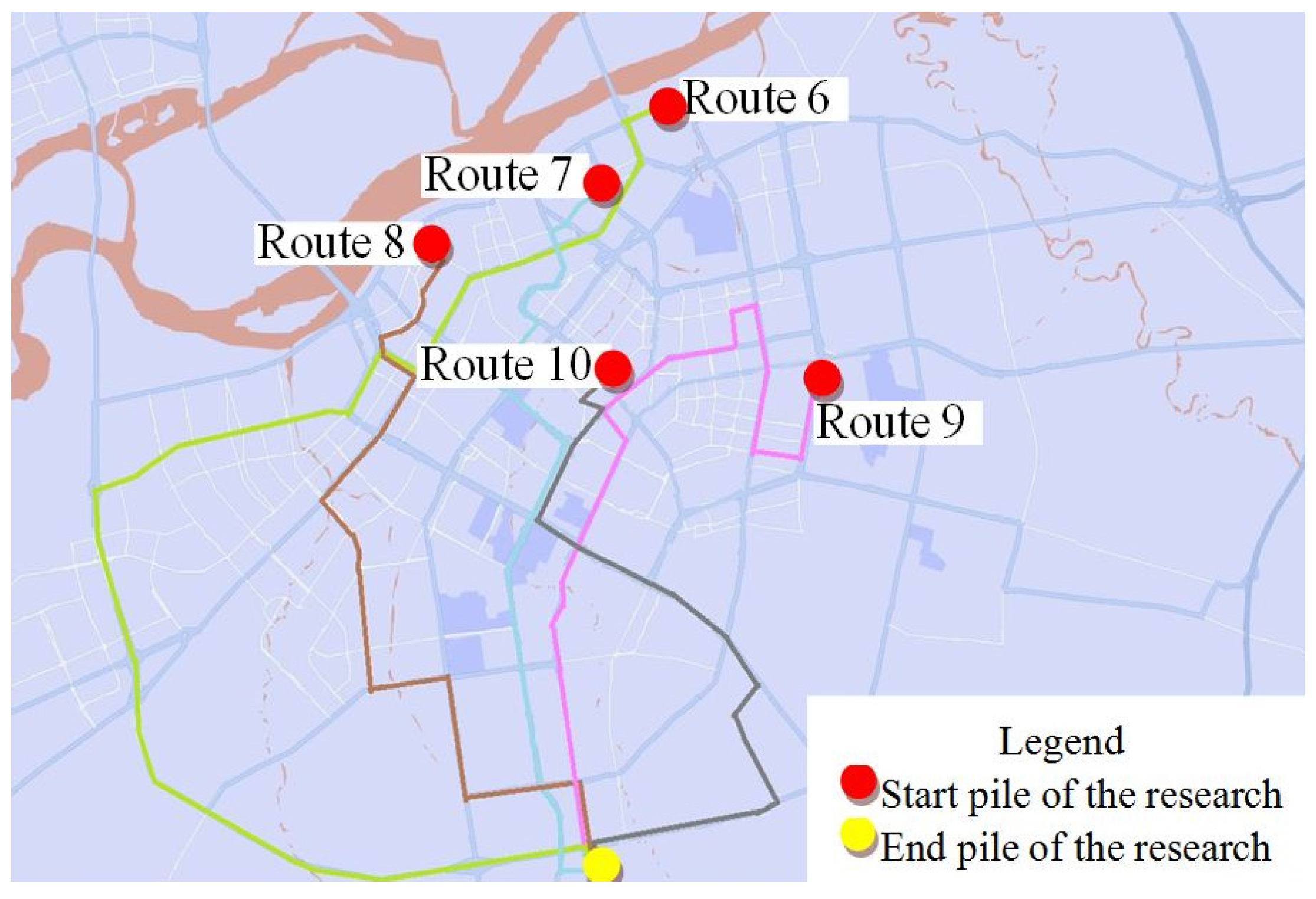
2.3. Experimental Routes and Scenarios
2.4. Procedure
2.5. Data Collection and Analysis
2.5.1. Speed
2.5.2. Vehicle Clearance
3. Results
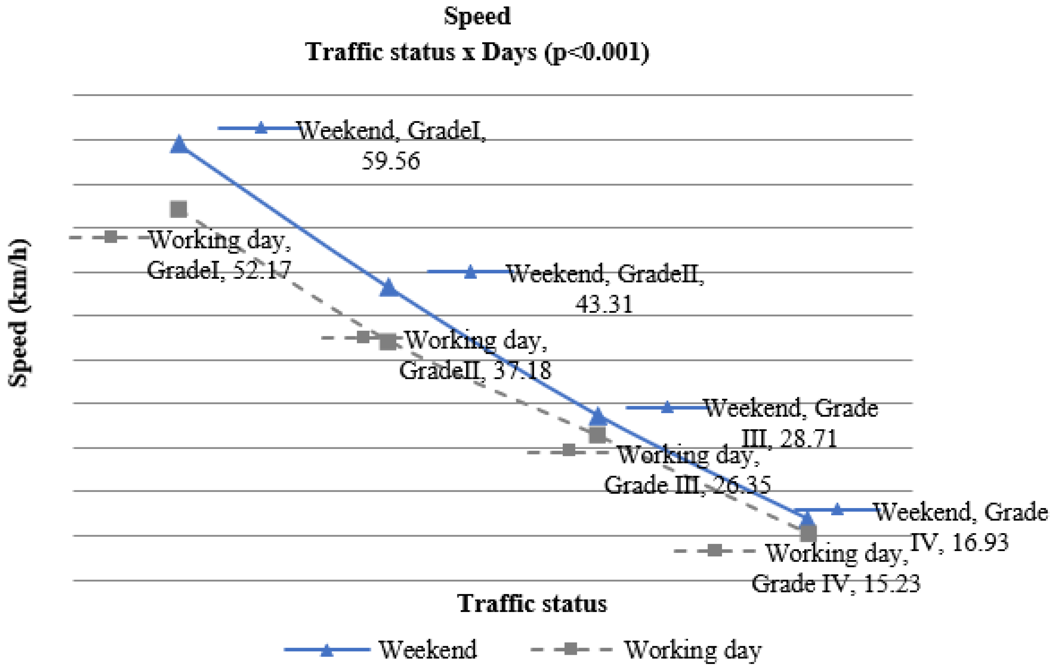
3.1. Speed
3.1.1. Working Days and Weekend
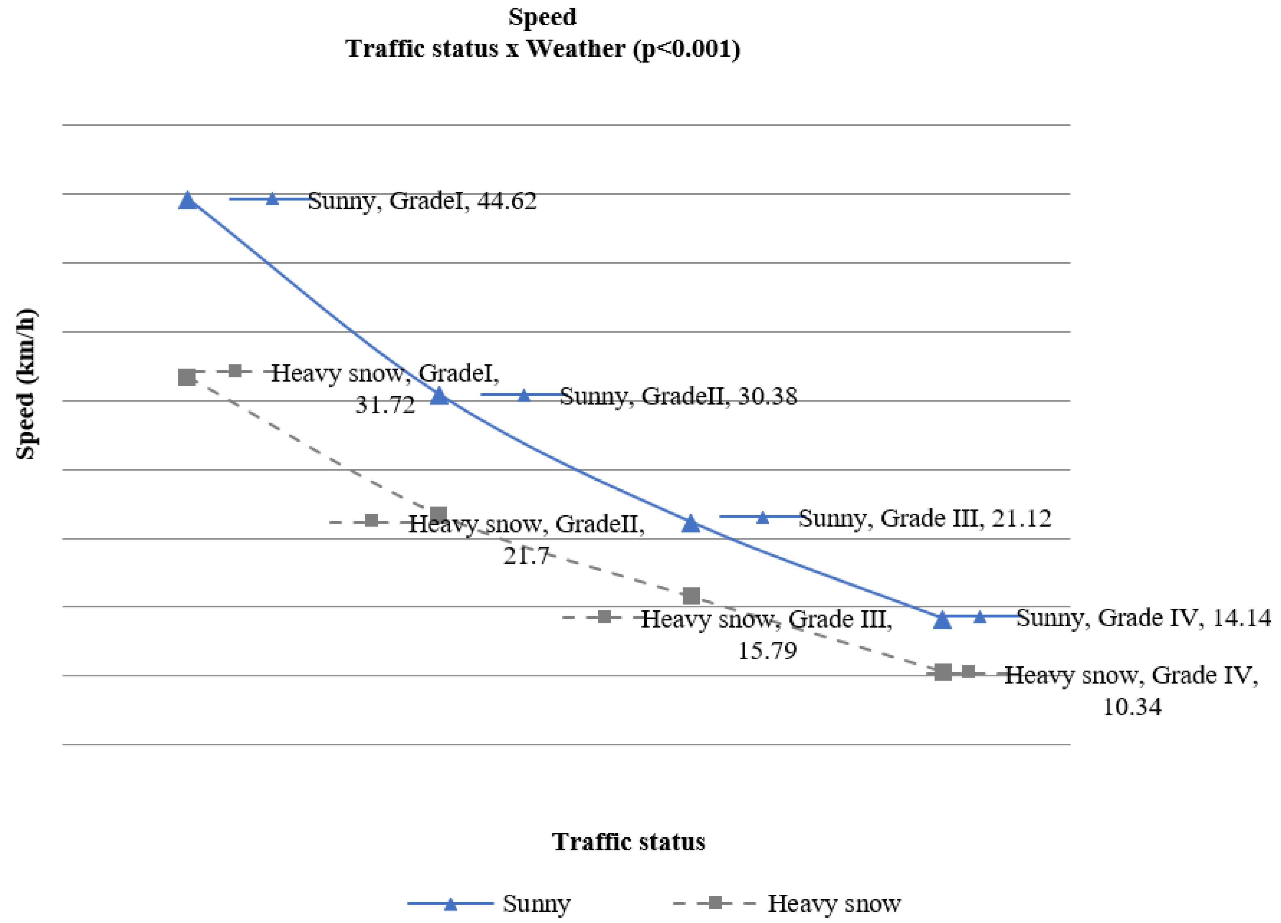
3.1.2. Weather Condition
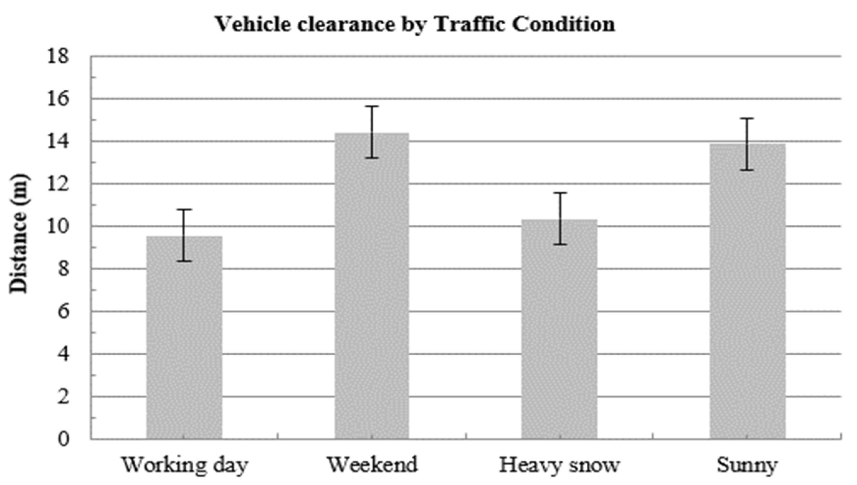
3.2. Vehicle-to-VehicleDistance
4. Discussion and Conclusions
4.1. Speed
4.2. Vehicle-to-VehicleDistance
5. Limitations and Further Research
Author Contributions
Funding
Institutional Review Board Statement
Informed Consent Statement
Data Availability Statement
Conflicts of Interest
References
- Mollu, K.; Biesbrouck, M.; Van Broeckhoven, L.; Daniëls, S.; Pirdavani, A.; Declercq, K.; Vanroelen, G.; Brijs, K.; Brijs, T. Priority rule signalization under two visibility conditions: Driving simulator study on speed and lateral position. Transp. Res. F 2018, 58, 156–166. [Google Scholar] [CrossRef]
- Liu, C.; Qiao, J.Y.; Jin, X. Study on route optimization of commute buses based on ant colony algorithm. Logist. Technol. 2013, 32, 278–280. [Google Scholar]
- Weng, C.W. One Company Work Commuter Car Path Problem Research Based on the Management Information System. Master’s Thesis, Shanghai Jiao Tong University, Shanghai, China, 2017. [Google Scholar]
- Gaodemap. Traffic Analysis Report of Q1 Major Cities in China in 2019; Institute of Sociology, Chinese Academy of Social Sciences, Intelligent Technology Laboratory of Urban Public Transport, 2019. Available online: https://www.takefoto.cn/viewnews-1762233.html (accessed on 14 February 2022).
- Li, J.; Lv, Y.B.; Ma, J.H.; Ren, Y. Factor analysis of customized bus attraction to commuters with different travel modes. Sustainability 2019, 11, 7065. [Google Scholar] [CrossRef] [Green Version]
- Chaudhary, M.L. Commuters’ perceptions on service quality of bus rapid transit systems: Evidence from the cities of Ahmedabad, Surat and Rajkot in India. Eur. Transp.-Trasp. Eur. 2020, 79. Available online: http://www.istiee.unict.it/sites/default/files/files/Paper%207%20n%2079.pdf (accessed on 14 February 2022).
- Suman, H.K.; Bolia, N.B.; Tiwari, G. Analysis of the factors influencing the use of public buses in Delhi. J. Urban Plan. Dev. 2016, 142, 04016003. [Google Scholar] [CrossRef]
- Yu, Q.; Zhang, H.; Li, W.; Song, X.; Yang, D.; Shibasaki, R. Mobile phone GPS data in urban customized bus: Dynamic line design and emission reduction potentials analysis. J. Clean. Prod. 2020, 272, 122471. [Google Scholar] [CrossRef]
- Yin, Y.H.; Yu, H.Z.N.; Wang, J.G. Research on characteristics of Beijing road traffic flow based on GIS. Highw. Eng. 2020, 45, 102–108. [Google Scholar]
- Zhao, X.H.; Ren, G.C.; Chen, C.; Rong, J.; Chang, X. Comprehensive effects of adverse weather on driver on driving simulation technology. J. Chongqing Jiaotong Univ. (Nat. Sci.) 2019, 38, 90–95. [Google Scholar]
- Maki, P.J. Adverse weather traffic signal timing. In Proceedings of the 69th Annual Meeting of the Institute of Transportation Engineers, Las Vegas, NV, USA, 1–4 August 1999. [Google Scholar]
- Liu, L.L.; Weng, J.C.; Rong, J. Study on traffic flow characteristics of urban expressway under snowfall. Traffic Inf. Saf. 2012, 30, 10–14. [Google Scholar]
- Wu, L.X.; Li, Y.X. Analysis on traffic flow characteristics of signalized intersections in Changchun under ice and snow conditions. Fujian Transp. Sci. Technol. 2019, 1, 116–118. [Google Scholar]
- Yao, Y.J.; Han, N.C.; Ma, T.B.; Zhan, Z.H. Measurement method of vehicle speed based on single loop-coil. Instrum. Tech. Sens. 2016, 6, 104–107. [Google Scholar]
- Liu, X.L.; Jiao, X.L.; Hu, Y.Z.; Hu, J.; Yu, T.T. Study on dynamic characteristics and coordinated control method of urban traffic flow. Traffic Enterpr. Manag. 2019, 34, 49–51. [Google Scholar]
- Shin, E.J. Commuter benefits programs: Impacts on mode choice, VMT, and spillover effects. Transp. Policy 2020, 94, 11–22. [Google Scholar] [CrossRef]
- Wang, J.; Zhang, M. Identifying the service areas and travel demand of the commuter customized bus based on mobile phone signaling data. J. Adv. Transp. 2021, 2021, 6934998. [Google Scholar] [CrossRef]
- Chen, L.; Ma, Z.; Li, Q.; Zhen, Q. Waiting decision behavior of commuters for bus transits based on prospect theory. J. Transp. Eng. A Syst. 2021, 147, 04021008. [Google Scholar] [CrossRef]
- Wang, Z.B.; Wang, S.C.; Lian, H.T. A route-planning method for long-distance commuter express bus service based on OD estimation from mobile phone location data: The case of the Changping Corridor in Beijing. Public Transp. 2021, 13, 101–125. [Google Scholar] [CrossRef]
- Qiu, G.; Song, R.; He, S. Clustering passenger trip data for the potential passenger investigation and line design of customized commuter bus. IEEE Trans. Intell. Transp. Syst. 2019, 20, 3351–3360. [Google Scholar] [CrossRef]
- Zhang, L.; Ma, J.; Liu, P.; Zhang, G. Study on the risk evaluation of commuter buses in coal enterprises based on GAHP. In Proceedings of the 19th COTA International Conference of Transportation Professionals (CICTP)—Transportation in China 2025, Nanjing, China, 6–8 July 2019; pp. 3500–3511. [Google Scholar]
- Lyman, C.; Campbell, N.; Gonzales, E.J. Modeling the effect of new commuter bus service on demand and impact on greenhouse gas emissions: Application to Greater Boston. Transp. Res. Rec. 2019, 2673, 125–138. [Google Scholar] [CrossRef]
- Antin, J.; Lee, S.; Hankey, J. Design of the in-Vehicle Driving Behavior and Crash Risk Study: In Support of the SHRP 2 Naturalistic Driving Study; Transportation Research Board of the National Academies: Washington, DC, USA, 2011. [Google Scholar]
- Feng, S.M.; Huang, Q.J.; Zhang, Y.; Zhao, H. Driver’s perception-decision-control model. J. Transp. Syst. Eng. Inf. Technol. 2021, 21, 41–47. [Google Scholar]
- Shao, Y.M.; Xu, J.; Li, B.W.; Yang, K. Modeling the speed choice behaviors of drivers on mountainous roads with complicated shapes. Adv. Mech. Eng. 2015, 7, 862610. [Google Scholar] [CrossRef]
- Jin, X.Q.; Wang, L.J.; Shao, Y. Headway spacing for different traffic flows. J. Dalian Jiaotong Univ. 2014, 35, 33–36. [Google Scholar]
- Ma, Y.L.; Leng, X.; Hu, B.Y. Influence of in-vehicle information system operation on driver action distraction. J. Transp. Syst. Eng. Inf. Technol. 2015, 15, 204–209. [Google Scholar]
- Cheng, G.Z.; Mo, X.Y.; Mao, C.Y. Urban road traffic safety evaluation method under the condition of ice and snowpavement. J. Transp. Syst. Eng. Inf. Technol. 2011, 11, 130–134. [Google Scholar]
- Fisher, D.L.; Rizzo, M.; Caired, J.K.; Rizzo, M.; Lee, J.D. Handbook of Driving Simulation for Engineering, Medicine, and Psychology; CRC Press Taylor & Francis Group: Boca Raton, FL, USA, 2011. [Google Scholar]
- Available online: https://www.qcwxjs.com (accessed on 15 November 2021).
- Ren, H.G.; Wang, Z.B.; Chen, Y.Y. Optimal express bus routes design with limited-stop services for long-distance commuters. Sustainability 2020, 12, 1669. [Google Scholar] [CrossRef] [Green Version]
- Liu, C.X.; Zhang, Y.P.; Cheng, G.Z. Traffic flow characteristic analysis of signal intersection on the ice and snow condition. J. Wuhan Univ. Technol. 2014, 38, 806–815. [Google Scholar]
- Montella, A. Identifying crash contributory factors at urban roundabouts and usingassociation rules to explore their relationships to different crash types. Accid. Anal. Prev. 2011, 43, 1451–1463. [Google Scholar] [CrossRef]
- Xu, C.; Liu, P.; Wang, W.; Li, Z. Evaluation of the impacts of traffic states on crash risks on freeways. Accid. Anal. Prev. 2012, 47, 162–171. [Google Scholar] [CrossRef]
- Liu, Z.Q.; Zhang, K.D.; Ni, J. Analysis and identification of drivers’ difference in car-following condition based on naturalisticdrivingdata. J. Transp. Syst. Eng. Inf. Technol. 2021, 21, 48–55. [Google Scholar]
- Fung, N.C.; Wallace, B.; Chan, A.D.C.; Goubran, R.; Porter, M.M.; Marshall, S.; Knoefel, F. Driver Identification Using Vehicle Acceleration and Deceleration Events from Naturalistic Driving of Older Drivers International Symposium on Medical Measurements and Applications (Memea); IEEE Publications: Rochester, MN, USA, 2017; pp. 33–38. [Google Scholar] [CrossRef]


| Grade I (Free Flow) | Grade II (Intermediate Range of Steady Flow) | Grade III (Lower Half of Steady Flow) | Grade IV (Unsteady Flow) | |
|---|---|---|---|---|
| Traffic volume (pcu/30 m ahead) | ≤3 | (3, 7) | [7, 11) | ≥11 |
| V/C | ≤0.25 | (0.25, 0.53) | [0.53, 0.65) | ≥0.65 |
| Evaluation score | ≤1.25 | (1.25, 2.25) | [2.25, 3.50) | ≥3.50 |
| Device | Location | Function | Data Collection | Result |
|---|---|---|---|---|
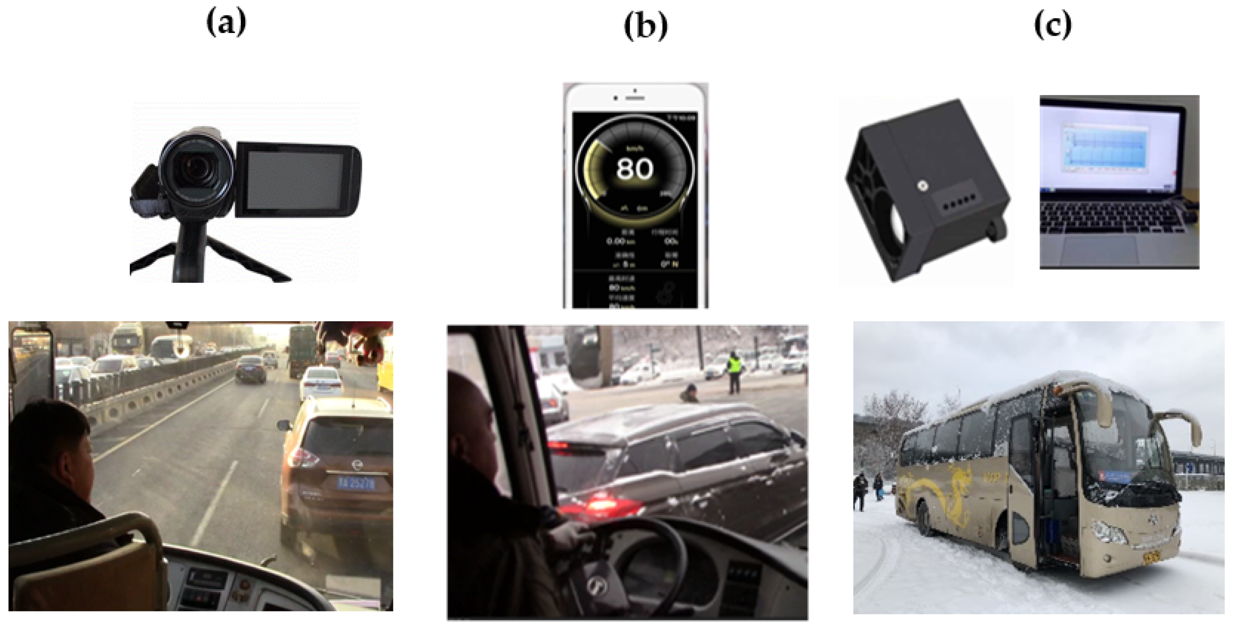
| Camera (Canon HF 806) | Inside bus behind the driver | Recording | Weather and road environment Manipulation behavior | Naturalistic driving data |
| Smartphone (iPhone 8 plus) | First-row seats inside the bus | GPS Speed (an App) Screen recording | Measuring vehicle operation data in real time (speed, mileage, etc.) Recording vehicle operation data of the entire rout | |
| Laser distance sensor (SK-Z-5) and laptop (Lenovo) | In the middle of the front outside the bus and the laptop inside | Measuring Recording | Displaying real-time vehicle spacing curve and data Recording vehicle spacing curve and data of the entire route |
| Effect | Traffic Status | Traffic Scenarios | Traffic Status | Traffic Scenarios | Estimate | Standard Error | DF | t-Value | Pr > |t| |
|---|---|---|---|---|---|---|---|---|---|
| Traffic status × day | Grade I | Weekend | Grade I | Working day | 7.71 | 4.43 | 58 | 17.58 | <0.0001 |
| Grade I | Weekend | Grade I | Working day | 5.84 | 2.34 | 58 | 16.35 | <0.0001 | |
| Grade III | Weekend | Grade III | Working day | 2.35 | 1.89 | 58 | 9.55 | <0.0001 | |
| Grade IV | Weekend | Grade IV | Working day | 1.69 | 1.71 | 58 | 7.57 | <0.0001 | |
| Traffic status × day | Grade I | Working day | Grade I | Working day | 13.68 | 3.51 | 58 | 25.58 | <0.0001 |
| Grade I | Working day | Grade III | Working day | 24.98 | 3.73 | 58 | 51.46 | <0.0001 | |
| Grade I | Working day | Grade IV | Working day | 36.10 | 4.08 | 58 | 67.95 | <0.0001 | |
| Grade I | Working day | Grade III | Working day | 10.89 | 1.53 | 58 | 46.53 | <0.0001 | |
| Grade I | Working day | Grade IV | Working day | 22.22 | 1.96 | 58 | 74.04 | <0.0001 | |
| Grade III | Working day | Grade IV | Working day | 11.11 | 2.01 | 58 | 42.41 | <0.0100 | |
| Traffic status × day | Grade I | Weekend | Grade I | Weekend | 15.81 | 3.19 | 58 | 32.51 | <0.0001 |
| Grade I | Weekend | Grade III | Weekend | 31.08 | 3.14 | 58 | 75.99 | <0.0001 | |
| Grade I | Weekend | Grade IV | Weekend | 42.86 | 3.16 | 58 | 104.22 | <0.0001 | |
| Grade I | Weekend | Grade III | Weekend | 14.54 | 1.89 | 58 | 50.44 | <0.0001 | |
| Grade I | Weekend | Grade IV | Weekend | 26.38 | 1.77 | 58 | 97.62 | <0.0001 | |
| Grade III | Weekend | Grade IV | Weekend | 11.78 | 0.77 | 58 | 116.66 | <0.0001 |
| Effect | Traffic Status | Weather | Traffic Status | Weather | Estimate | Standard Error | DF | t-Value | Pr > |t| |
|---|---|---|---|---|---|---|---|---|---|
| Traffic status × weather | Grade I | Sunny | Grade I | HS | 6.98 | 2.47 | 58 | 28.49 | <0.0001 |
| Grade I | Sunny | Grade I | HS | 4.14 | 1.71 | 58 | 15.80 | <0.0001 | |
| Grade III | Sunny | Grade III | HS | 1.44 | 1.12 | 58 | 9.90 | <0.0001 | |
| Grade IV | Sunny | Grade IV | HS | 1.81 | 0.95 | 58 | 14.65 | <0.0001 | |
| Traffic status × weather | Grade I | HS | Grade I | HS | 9.79 | 2.19 | 58 | 34.34 | <0.0001 |
| Grade I | HS | Grade III | HS | 15.70 | 2.05 | 58 | 58.90 | <0.0001 | |
| Grade I | HS | Grade IV | HS | 21.15 | 2.12 | 58 | 76.69 | <0.0001 | |
| Grade I | HS | Grade III | HS | 5.91 | 1.22 | 58 | 37.31 | <0.0001 | |
| Grade I | HS | Grade IV | HS | 11.37 | 1.16 | 58 | 75.54 | <0.0001 | |
| Grade III | HS | Grade IV | HS | 5.46 | 0.98 | 58 | 42.45 | <0.0001 | |
| Traffic status × weather | Grade I | Sunny | Grade I | Sunny | 12.39 | 2.11 | 58 | 38.37 | <0.0001 |
| Grade I | Sunny | Grade III | Sunny | 21.61 | 2.02 | 58 | 82.24 | <0.0001 | |
| Grade I | Sunny | Grade IV | Sunny | 26.71 | 1.96 | 58 | 104.76 | <0.0001 | |
| Grade I | Sunny | Grade III | Sunny | 8.75 | 1.18 | 58 | 48.52 | <0.0001 | |
| Grade I | Sunny | Grade IV | Sunny | 13.95 | 1.19 | 58 | 77.13 | <0.0001 | |
| Grade III | Sunny | Grade IV | Sunny | 5.09 | 0.56 | 58 | 68.83 | <0.0001 |
Publisher’s Note: MDPI stays neutral with regard to jurisdictional claims in published maps and institutional affiliations. |
© 2022 by the authors. Licensee MDPI, Basel, Switzerland. This article is an open access article distributed under the terms and conditions of the Creative Commons Attribution (CC BY) license (https://creativecommons.org/licenses/by/4.0/).
Share and Cite
Huang, Q.; Feng, S.; Zhang, G.; Zhang, Y.; Harumain, Y.A.S. Commuter Bus Operation Rules under Two Traffic Scenarios and Two Weather Conditions: Naturalistic Driving Study on Vehicle Speed and Clearance. Sustainability 2022, 14, 2473. https://doi.org/10.3390/su14042473
Huang Q, Feng S, Zhang G, Zhang Y, Harumain YAS. Commuter Bus Operation Rules under Two Traffic Scenarios and Two Weather Conditions: Naturalistic Driving Study on Vehicle Speed and Clearance. Sustainability. 2022; 14(4):2473. https://doi.org/10.3390/su14042473
Chicago/Turabian StyleHuang, Qiuju, Shumin Feng, Guosheng Zhang, Yu Zhang, and Yong Adilah Shamsul Harumain. 2022. "Commuter Bus Operation Rules under Two Traffic Scenarios and Two Weather Conditions: Naturalistic Driving Study on Vehicle Speed and Clearance" Sustainability 14, no. 4: 2473. https://doi.org/10.3390/su14042473
APA StyleHuang, Q., Feng, S., Zhang, G., Zhang, Y., & Harumain, Y. A. S. (2022). Commuter Bus Operation Rules under Two Traffic Scenarios and Two Weather Conditions: Naturalistic Driving Study on Vehicle Speed and Clearance. Sustainability, 14(4), 2473. https://doi.org/10.3390/su14042473