
Urban Quality of Life and Production Amenity in Chinese Cities


Abstract
:1. Introduction
1.1. Background
1.2. Literature Review
2. Methods
2.1. Model
2.2. Regressions of Wage Differentials and Housing Costs Differentials
2.3. Variables and Data
3. Measurement of Urban Quality of Life and Production Amenity
3.1. Measurement of Urban Quality of Life
3.2. Robustness Test
3.2.1. Comparison with the Results Using the U.S. Parameters
3.2.2. Comparison with Popular Rankings
3.3. Measurement of Production Amenity
4. Characteristic Facts of Urban Quality of Life and Production Amenity
4.1. Characteristic Facts of Urban Quality of Life
4.2. Characteristic Facts of Production Amenity
5. Influencing Factors
5.1. Influencing Factors of Urban Quality of Life
5.2. Influencing Factors of Production Amenity
5.3. Discussion
6. Conclusions
Author Contributions
Funding
Institutional Review Board Statement
Informed Consent Statement
Data Availability Statement
Conflicts of Interest
Appendix A. Parameter Assignment of the Model
Appendix A.1. The Income Shares of Residents
- (1)
- The expenditure shares of residents
- (2)
- The shares of factor costs for firms

| Variables | Parameters in This Paper | Parameters in Albouy 2016 | |
|---|---|---|---|
| Share of local goods consumption | 0.3 | 0.36 | |
| Labor income share | 0.74 | 0.75 | |
| Land income share | 0.18 | 0.1 | |
| Land cost share of traded goods | 0.025 | 0.025 | |
| Labor cost share of traded goods | 0.895 | 0.825 | |
| Land cost share of local goods | 0.542 | 0.233 | |
| Labor cost share of local goods | 0.378 | 0.617 | |
| Wage income tax rate | 0.092 | 0.361 | |
Appendix A.2. The Selection of Tax Rate
Appendix B. The Estimations of Wage and Housing Price Differentials
| Wage Level (Logarithm of Hourly Wage) | (1) | (2) | (3) | (4) | |
|---|---|---|---|---|---|
| Gender (0 for male) | −0.3001 *** | −0.3024 *** | −0.2534 *** | −0.5906 | |
| (0.0079) | (0.0079) | (0.0081) | (0.3753) | ||
| Education level (0 for primary school or under) | Junior | 0.0363 *** | 0.0309 ** | 0.0445 *** | 0.0305 * |
| (0.0143) | (0.0143) | (0.014) | (0.018) | ||
| High | 0.1555 *** | 0.1435 *** | 0.1582 *** | 0.1188 *** | |
| (0.0157) | (0.0162) | (0.016) | (0.0204) | ||
| College | 0.3816 *** | 0.3604 *** | 0.3587 *** | 0.3133 *** | |
| (0.0184) | (0.0194) | (0.0195) | (0.0251) | ||
| Undergraduate | 0.5858 *** | 0.5595 *** | 0.5416 *** | 0.4597 *** | |
| (0.0196) | (0.0209) | (0.0217) | (0.0279) | ||
| Postgraduate and above | 1.0137 *** | 0.9802 *** | 0.9530 *** | 0.8947 *** | |
| (0.04) | (0.0407) | (0.041) | (0.0532) | ||
| Work experience | Work experience | 0.031 *** | 0.0269 *** | 0.0267 *** | 0.0321*** |
| (0.0013) | (0.0016) | (0.0015) | (0.002) | ||
| Work experience square | −0.0006 *** | −0.0006 *** | −0.0006 *** | −0.0007 *** | |
| (0.0000) | (0.0000) | (0.0000) | (0.0000) | ||
| Marital status (0 for Single) | Married | 0.0574 *** | 0.0505 *** | 0.0769 *** | |
| (0.0145) | (0.0142) | (0.0181) | |||
| Divorced | 0.0542 * | 0.0397 | 0.0066 | ||
| (0.0319) | (0.0312) | (0.0399) | |||
| Widowed | −0.0081 | 0.0038 | −0.0079 | ||
| (0.0485) | (0.0475) | (0.0711) | |||
| Physical condition (0 for Bad) | Good | 0.1714 *** | 0.1548 *** | 0.1695 *** | |
| (0.0306) | (0.0300) | (0.0351) | |||
| Median | 0.1032 *** | 0.0951 *** | 0.1042 *** | ||
| (0.0318) | (0.0312) | (0.0368) | |||
| Ethnic minorities (0 for Han) | −0.0571 | −0.0416 | −0.1060 ** | ||
| (0.0378) | (0.0371) | (0.0504) | |||
| Household register (0 for Rural) | Urban | 0.0244 ** | 0.0340 *** | 0.0302 ** | |
| (0.0102) | (0.0101) | (0.0129) | |||
| Others | 0.0102 | 0.0160 | 0.0079 | ||
| (0.0148) | (0.0145) | (0.0175) | |||
| City | Controlled | Controlled | Controlled | Controlled | |
| Industry | Controlled | Controlled | |||
| Gender cross | Controlled | ||||
| Constant | 2.2487 *** | 2.0839 *** | 1.7800 *** | 1.9043 *** | |
| (0.0197) | (0.0360) | (0.1850) | (0.2387) | ||
| Obs. | 20,030 | 20,030 | 20,030 | 20,030 | |
| R2 | 0.2568 | 0.2601 | 0.2914 | 0.2975 | |
| Housing Price | (1) | (2) | |||
|---|---|---|---|---|---|
| Housing age | −0.0066 *** | (0.0007) | −0.0076 *** | (0.0008) | |
| Areas | 0.0065 *** | (0.0002) | 0.0064 *** | (0.0002) | |
| Room numbers | Bedroom | 0.0897 *** | (0.0075) | 0.0863 *** | (0.0073) |
| Living room | 0.0839 *** | (0.0105) | 0.0747 *** | (0.0103) | |
| Washing room | 0.0099 | (0.0096) | 0.0288 *** | (0.0095) | |
| Housing type (0 for Ordinary House) | Villa | −0.1473 *** | (0.0401) | ||
| Apartment | −0.3773 *** | (0.0317) | |||
| Others | 0.1627 | (0.1181) | |||
| Orientation (0 for South-North) | South, southeast, southwest | −0.0167 ** | (0.0085) | ||
| East or West | 0.0083 | (0.0195) | |||
| North, northeast, northwest | 0.1071 *** | (0.0287) | |||
| Floors (0 for Low) | Median | −0.0176 * | (0.0095) | ||
| High | −0.0429 *** | (0.0096) | |||
| Other | −0.0428 ** | (0.0187) | |||
| Decoration (0 for Rough) | Simple | 0.0102 | (0.0136) | ||
| Refined | 0.0869 *** | (0.0093) | |||
| Luxurious | 0.1909 *** | (0.0178) | |||
| Constant | 3.3450 *** | (0.0205) | 3.3474 *** | (0.0231) | |
| Obs. | 7400 | 7400 | |||
| R2 | 0.7548 | 0.7675 | |||
Appendix C. Calculation Results of the Measurement of Urban QOL and Production Amenity
| City | Pop. | GDP per Capita | |||||
|---|---|---|---|---|---|---|---|
| Chongqing | 0.0363 | 0.01 | 0.0326 | −0.0204 | −0.0132 | 3336.6 | 38,914 |
| Beijing | 0.2479 | 1.71 | 0.3037 | 0.3468 | 0.4281 | 1287.7 | 87,475 |
| Zhoukou | −0.116 | 0.05 | −0.0996 | 0.0926 | 0.0716 | 1234.0 | 17,734 |
| Chengdu | 0.085 | 0.66 | 0.1076 | 0.14 | 0.1693 | 1168.3 | 57,624 |
| Fuyang | −0.1936 | −0.08 | −0.1746 | 0.1047 | 0.0662 | 1032.8 | 12,616 |
| Xuzhou | −0.0946 | 0.14 | −0.0763 | 0.105 | 0.0898 | 983.6 | 46,877 |
| Shangqiu | −0.0708 | −0.16 | −0.0703 | −0.0006 | −0.0172 | 930.5 | 19,029 |
| Weifang | −0.011 | 0.13 | −0.0034 | 0.0452 | 0.0457 | 878.2 | 43,681 |
| Jining | −0.13 | 0.02 | −0.1135 | 0.0926 | 0.0682 | 847.0 | 39,165 |
| Wuhan | 0.0881 | 0.63 | 0.1089 | 0.1294 | 0.1586 | 824.5 | 79,482 |
| Yancheng | 0.0005 | 0.1 | 0.0057 | 0.0309 | 0.0331 | 821.6 | 43,172 |
| Guangzhou | 0.1348 | 1.01 | 0.1691 | 0.2126 | 0.2584 | 818.4 | 105,909 |
| Hengyang | 0.0122 | −0.19 | 0.0014 | −0.064 | −0.0655 | 798.4 | 27,258 |
| Qingdao | 0.0353 | 0.45 | 0.0538 | 0.1124 | 0.1282 | 768.0 | 82,680 |
| Nantong | −0.0029 | 0.25 | 0.01 | 0.0772 | 0.0816 | 765.0 | 62,506 |
| Zhengzhou | 0.0353 | 0.43 | 0.0527 | 0.1063 | 0.1216 | 762.8 | 62,054 |
| Nanchong | −0.0133 | −0.17 | −0.0203 | −0.0427 | −0.0487 | 757.9 | 18,757 |
| Maoming | −0.0891 | −0.21 | −0.0888 | −0.0029 | −0.024 | 755.1 | 32,678 |
| Xinyang | 0.0113 | −0.12 | 0.004 | −0.0432 | −0.0435 | 747.5 | 22,347 |
| Shenyang | −0.0695 | 0.33 | −0.0449 | 0.1444 | 0.1377 | 723.7 | 80,480 |
| Luoyang | −0.2116 | −0.01 | −0.1868 | 0.138 | 0.0976 | 710.4 | 45,316 |
| Lu’an | −0.1432 | −0.09 | −0.1306 | 0.0684 | 0.0394 | 709.9 | 16,248 |
| Hefei | 0.0545 | 0.42 | 0.069 | 0.0895 | 0.1082 | 708.3 | 55,186 |
| Huanggang | −0.027 | −0.18 | −0.033 | −0.0369 | −0.0457 | 685.7 | 19,220 |
| Changsha | 0.0375 | 0.25 | 0.0454 | 0.0495 | 0.0616 | 658.6 | 89,903 |
| Yantai | −0.1264 | 0.18 | −0.1021 | 0.1391 | 0.1187 | 651.0 | 75,672 |
| Suzhou | 0.2633 | 0.9 | 0.2768 | 0.0943 | 0.1623 | 645.1 | 114,029 |
| Nanjing | 0.2133 | 1.04 | 0.2396 | 0.1681 | 0.2294 | 637.4 | 88,525 |
| Changde | −0.0096 | −0.09 | −0.0129 | −0.0205 | −0.0241 | 627.4 | 35,475 |
| Anqing | −0.0361 | −0.17 | −0.0402 | −0.026 | −0.0362 | 619.5 | 25,592 |
| Yongzhou | 0.0246 | −0.26 | 0.0086 | −0.0946 | −0.0951 | 617.6 | 20,239 |
| Xinxiang | −0.0549 | 0.19 | −0.0387 | 0.0947 | 0.0882 | 614.8 | 28,598 |
| Qujing | −0.175 | −0.28 | −0.168 | 0.0334 | −0.0055 | 613.6 | 23,661 |
| Bozhou | −0.0728 | −0.05 | −0.0665 | 0.0343 | 0.0196 | 608.4 | 14,642 |
| Jinan | −0.1122 | 0.59 | −0.0691 | 0.2527 | 0.2433 | 607.9 | 69,444 |
| Liaocheng | −0.1045 | −0.01 | −0.0925 | 0.0667 | 0.0466 | 599.3 | 36,573 |
| Xiangyang | −0.1346 | −0.12 | −0.1244 | 0.0545 | 0.0265 | 593.8 | 45,167 |
| Dalian | −0.0394 | 0.23 | −0.0231 | 0.0958 | 0.093 | 589.4 | 102,922 |
| Dezhou | −0.1633 | 0.18 | −0.1348 | 0.163 | 0.1356 | 576.8 | 39,710 |
| Yueyang | 0.1045 | −0.04 | 0.0901 | −0.0814 | −0.0623 | 571.1 | 39,968 |
| Huaian | −0.0051 | 0.02 | −0.0036 | 0.0082 | 0.0076 | 545.0 | 39,992 |
| Mianyang | 0.0055 | 0 | 0.0048 | −0.004 | −0.003 | 544.4 | 27,056 |
| Kaifeng | −0.1559 | 0.04 | −0.1351 | 0.1171 | 0.0883 | 543.9 | 25,922 |
| Kunming | −0.0549 | 0.12 | −0.0424 | 0.0724 | 0.0643 | 543.8 | 46,256 |
| Shantou | −0.0471 | −0.07 | −0.0452 | 0.0091 | −0.0014 | 531.2 | 26,231 |
| Xiaogan | −0.0625 | −0.22 | −0.0661 | −0.0248 | −0.0411 | 527.9 | 20,934 |
| Meizhou | 0.067 | −0.16 | 0.0511 | −0.0917 | −0.0821 | 519.5 | 17,425 |
| Yuncheng | −0.2842 | −0.26 | −0.2631 | 0.1124 | 0.0532 | 518.1 | 20,628 |
| Taizhou | 0.0312 | −0.15 | 0.0197 | −0.0672 | −0.0643 | 506.7 | 58,378 |
| Xuchang | −0.1564 | −0.08 | −0.1417 | 0.0803 | 0.0489 | 494.1 | 39,947 |
| Yiyang | −0.0292 | −0.37 | −0.0443 | −0.0925 | −0.1055 | 480.3 | 23,572 |
| Wuxi | 0.206 | 0.72 | 0.2173 | 0.0781 | 0.1316 | 469.0 | 117,357 |
| Chenzhou | 0.0043 | −0.24 | −0.0081 | −0.0742 | −0.0781 | 461.9 | 32,848 |
| Yangzhou | −0.0182 | 0.07 | −0.0125 | 0.0337 | 0.0316 | 459.2 | 65,692 |
| Loudi | −0.006 | −0.28 | −0.0191 | −0.0788 | −0.0855 | 436.8 | 26,367 |
| Zibo | −0.0947 | −0.01 | −0.0838 | 0.0602 | 0.0419 | 423.8 | 77,876 |
| Puyang | −0.2818 | −0.11 | −0.2537 | 0.1548 | 0.099 | 419.0 | 27,654 |
| Yichang | −0.0177 | 0.12 | −0.0097 | 0.0476 | 0.0466 | 398.9 | 61,517 |
| Zhuzhou | 0.0814 | −0.23 | 0.0601 | −0.1239 | −0.113 | 393.6 | 45,235 |
| Wuhu | −0.0234 | 0.09 | −0.0163 | 0.0417 | 0.0389 | 384.4 | 48,742 |
| Binzhou | 0.0035 | 0.22 | 0.0143 | 0.0648 | 0.07 | 380.8 | 52,591 |
| Suining | −0.0501 | −0.39 | −0.0635 | −0.083 | −0.1003 | 379.4 | 20,908 |
| Lvliang | −0.2575 | −0.35 | −0.2442 | 0.0671 | 0.0112 | 376.2 | 32,709 |
| Foshan | 0.1144 | 0.3 | 0.1158 | 0.0144 | 0.0422 | 376.2 | 91,259 |
| Tianshui | −0.1964 | −0.34 | −0.1898 | 0.0297 | −0.0144 | 374.5 | 12,593 |
| Jiaozuo | −0.1463 | 0.03 | −0.1273 | 0.1068 | 0.0796 | 368.6 | 44,029 |
| Bengbu | −0.0825 | −0.03 | −0.0741 | 0.0462 | 0.0299 | 366.6 | 27,999 |
| Taiyuan | −0.1546 | 0.23 | −0.1247 | 0.1714 | 0.1466 | 365.4 | 54,440 |
| Leshan | −0.0496 | −0.41 | −0.0642 | −0.0899 | −0.1075 | 354.8 | 30,386 |
| Anshan | −0.0874 | −0.3 | −0.0919 | −0.0318 | −0.0544 | 351.0 | 69,211 |
| Meishan | −0.0402 | −0.14 | −0.0422 | −0.0139 | −0.0242 | 350.6 | 26,168 |
| Chaoyang | −0.1883 | −0.4 | −0.1858 | 0.0057 | −0.0381 | 340.8 | 30,765 |
| Zigong | −0.0895 | −0.4 | −0.0989 | −0.0609 | −0.0859 | 327.8 | 32,787 |
| Jinzhong | −0.2048 | −0.13 | −0.1865 | 0.0992 | 0.0578 | 324.1 | 30,093 |
| Lanzhou | −0.1544 | 0.28 | −0.122 | 0.1864 | 0.1626 | 322.4 | 43,175 |
| Datong | −0.2572 | −0.39 | −0.2461 | 0.0539 | −0.0029 | 319.1 | 27,815 |
| Xinzhou | −0.2282 | −0.41 | −0.2211 | 0.0314 | −0.0201 | 310.1 | 20,081 |
| Jinzhou | −0.0977 | −0.14 | −0.0929 | 0.0237 | 0.0024 | 308.1 | 40,002 |
| Jingmen | −0.0412 | −0.17 | −0.0449 | −0.0248 | −0.0361 | 302.1 | 37,649 |
| Xianning | −0.0422 | −0.3 | −0.0519 | −0.0603 | −0.0742 | 296.6 | 30,791 |
| Yunfu | −0.1016 | −0.14 | −0.0962 | 0.0274 | 0.0054 | 286.6 | 22,539 |
| Huludao | −0.1203 | −0.3 | −0.121 | −0.0103 | −0.0393 | 280.7 | 27,709 |
| Shenzhen | 0.495 | 1.3 | 0.5004 | 0.0572 | 0.1772 | 277.8 | 123,247 |
| Dingxi | −0.1728 | −0.34 | −0.1692 | 0.0128 | −0.0269 | 273.7 | 8157 |
| Zhenjiang | 0.0571 | 0.45 | 0.0729 | 0.0976 | 0.1175 | 271.6 | 83,650 |
| Qingyang | −0.218 | −0.17 | −0.2002 | 0.0962 | 0.0515 | 262.1 | 23,882 |
| Weihai | −0.0744 | 0.06 | −0.0625 | 0.068 | 0.0551 | 253.7 | 92,148 |
| Huainan | −0.1072 | −0.06 | −0.0974 | 0.0535 | 0.0319 | 244.7 | 33,489 |
| Dandong | −0.1372 | −0.31 | −0.1363 | −0.0014 | −0.0337 | 240.8 | 42,171 |
| Lincang | −0.1085 | −0.31 | −0.1109 | −0.0198 | −0.0466 | 236.1 | 14,376 |
| Yingkou | −0.1038 | −0.4 | −0.1112 | −0.0501 | −0.0778 | 235.3 | 56,583 |
| Pingliang | −0.2333 | −0.31 | −0.2208 | 0.0633 | 0.0127 | 233.5 | 15,607 |
| Yuxi | −0.1651 | −0.05 | −0.1477 | 0.0961 | 0.0638 | 231.8 | 43,037 |
| Huaibei | −0.163 | −0.26 | −0.1565 | 0.0308 | −0.0054 | 220.1 | 29,278 |
| Fushun | −0.1144 | −0.48 | −0.1244 | −0.066 | −0.0972 | 219.7 | 58,512 |
| Jincheng | −0.1246 | −0.18 | −0.1187 | 0.0297 | 0.0024 | 217.9 | 44,257 |
| Fuxin | −0.1279 | −0.34 | −0.1297 | −0.0169 | −0.048 | 191.8 | 31,049 |
| Dongying | −0.1399 | 0.04 | −0.1209 | 0.1069 | 0.0812 | 185.7 | 145,395 |
| Liaoyang | −0.1307 | −0.38 | −0.134 | −0.0268 | −0.0592 | 181.4 | 53,877 |
| Baiyin | −0.2297 | −0.46 | −0.2253 | 0.0151 | −0.0378 | 177.6 | 25,274 |
| Shuozhou | −0.2182 | −0.43 | −0.2137 | 0.0162 | −0.034 | 173.0 | 58,205 |
| Zhangjiajie | −0.0725 | −0.19 | −0.0734 | −0.0092 | −0.0268 | 169.3 | 22,658 |
| Hebi | −0.168 | −0.17 | −0.1564 | 0.0613 | 0.0259 | 163.6 | 34,456 |
| Chizhou | −0.053 | −0.1 | −0.0519 | 0.0043 | −0.0079 | 161.7 | 29,471 |
| Yaan | −0.1125 | −0.26 | −0.1122 | −0.0037 | −0.0304 | 156.1 | 26,157 |
| Benxi | −0.1222 | −0.64 | −0.1395 | −0.1097 | −0.1457 | 153.8 | 64,459 |
| Huangshan | −0.0081 | −0.3 | −0.022 | −0.0835 | −0.091 | 147.7 | 28,773 |
| Yangquan | −0.2292 | −0.52 | −0.2274 | −0.001 | −0.0548 | 131.8 | 43,702 |
| Panzhihua | −0.0098 | −0.55 | −0.0361 | −0.1583 | −0.1712 | 111.8 | 60,391 |
| Ezhou | −0.1944 | −0.38 | −0.1901 | 0.0157 | −0.0289 | 105.3 | 53,192 |
| Jiuquan | −0.2252 | −0.37 | −0.2166 | 0.0405 | −0.0097 | 99.0 | 52,116 |
Appendix D. The Distribution of the City Sample
Appendix D.1. The Distribution of 111 Sample Cities in the Measurement
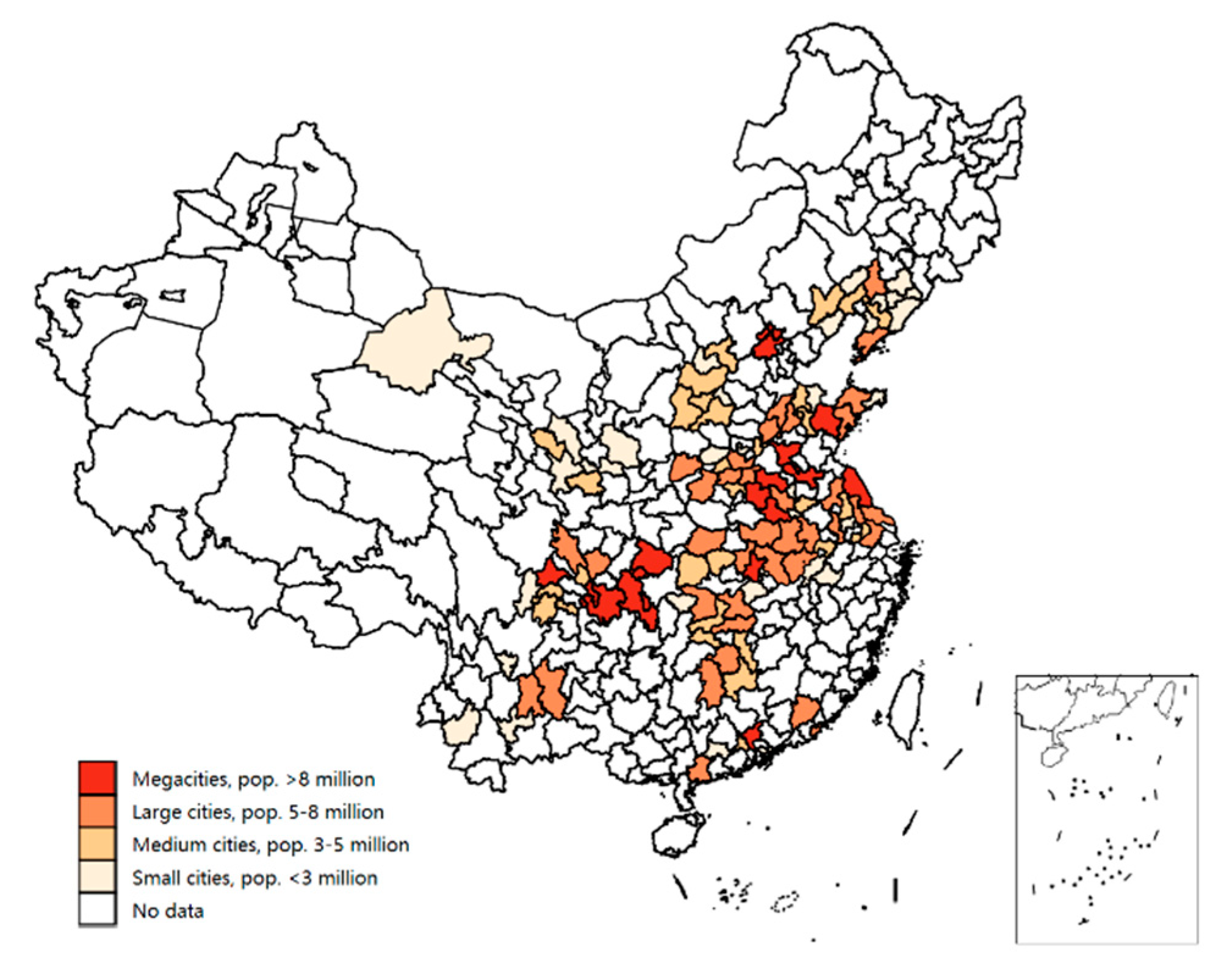
Appendix D.2. The Distribution of 281 Sample Cities in Characteristic Facts Section

Appendix E. The Influencing Factor Analysis Using Sub-Samples with Different Economic Aggregate
| Urban Characteristics | ||||||
|---|---|---|---|---|---|---|
| Developed | Developing | Underdeveloped | Developed | Developing | Underdeveloped | |
| x1 | 0.095 | −0.007 | 0.072 | −0.035 | 0.022 | 0.045 |
| (0.08) | (0.042) | (0.083) | (0.05) | (0.03) | (0.074) | |
| x2 | 0.295 | 0.091 | 0.302 | 0.144 | −0.181 * | −0.394 |
| (0.231) | (0.078) | (0.198) | (0.121) | (0.093) | (0.22) | |
| x3 | −0.066 | −0.086 ** | −0.09 | 0.12 *** | 0.047 * | 0.009 |
| (0.052) | (0.032) | (0.06) | (0.034) | (0.025) | (0.055) | |
| x4 | −0.016 | −0.015 | −0.008 | 0.048 * | 0.03 * | 0.029 |
| (0.041) | (0.014) | (0.024) | (0.024) | (0.014) | (0.024) | |
| x5 | −0.017 | 0.003 | −0.019 | −0.05 ** | −0.004 | 0.002 |
| (0.033) | (0.022) | (0.024) | (0.019) | (0.02) | (0.018) | |
| x6 | 0.005 | 0.022 | 0.019 | 0.024 | 0.023 | −0.045 |
| (0.037) | (0.023) | (0.047) | (0.041) | (0.025) | (0.036) | |
| x8 | 0.98 | 0.111 ** | 0.289 * | −0.866 | 0.048 | −0.031 |
| (1.355) | (0.051) | (0.152) | (0.836) | (0.045) | (0.167) | |
| x9 | −0.172 | −0.058 | −0.067 | 0.089 | 0.104 ** | 0.054 |
| (0.169) | (0.039) | (0.081) | (0.099) | (0.038) | (0.074) | |
| x10 | 0.004 | −0.012 | −0.013 | 0.034 | 0 | 0.038 * |
| (0.034) | (0.017) | (0.021) | (0.029) | (0.013) | (0.018) | |
| x11 | 0.106 *** | 0.056 | 0.018 | −0.046 | −0.07 | 0.075 |
| (0.028) | (0.042) | (0.047) | (0.027) | (0.049) | (0.053) | |
| x12 | −0.101 | −0.203 *** | −0.053 ** | 0.154 | 0.073 * | 0.069 *** |
| (0.149) | (0.047) | (0.02) | (0.11) | (0.036) | (0.02) | |
| x13 | −0.018 | −0.004 | −0.006 | 0.068 *** | 0.011 | 0.01 |
| (0.047) | (0.013) | (0.023) | (0.021) | (0.012) | (0.02) | |
| x14 | 0.017 | −0.011 | −0.001 | −0.057 ** | −0.012 | 0.005 |
| (0.038) | (0.007) | (0.016) | (0.023) | (0.007) | (0.015) | |
| x15 | 0.03 | 0.17 *** | 0.133 *** | −0.255 *** | −0.079 | −0.146 *** |
| (0.097) | (0.039) | (0.034) | (0.065) | (0.03) | (0.032) | |
| x16 | −0.011 | −0.048 * | −0.008 | 0.114 | 0.044 | 0.053 |
| (0.14) | (0.023) | (0.031) | (0.084) | (0.026) | (0.032) | |
| x17 | 0.003 | −0.016 | −0.023 | −0.044 ** | −0.049 *** | 0.015 |
| (0.035) | (0.013) | (0.026) | (0.018) | (0.013) | (0.019) | |
| x18 | −0.016 | 0.041 ** | 0.027 | 0.003 | −0.026 * | −0.006 |
| (0.036) | (0.014) | (0.026) | (0.033) | (0.014) | (0.024) | |
| x19 | −0.017 | 0.166 | −0.016 | 0.146 *** | 0.071 | −0.486 ** |
| (0.066) | (0.12) | (0.256) | (0.024) | (0.09) | (0.178) | |
| x20 | 0.025 | −0.012 | 0.002 | 0.06 | 0.013 | −0.036 |
| (0.042) | (0.036) | (0.042) | (0.044) | (0.028) | (0.038) | |
| x21 | 0.022 | 0.021 ** | −0.005 | 0.037 ** | 0.008 | 0.011 |
| (0.014) | (0.009) | (0.01) | (0.013) | (0.005) | (0.01) | |
| x22 | 0.029 | 0.008 | −0.036 | −0.035 *** | 0.012 | 0.028 |
| (0.035) | (0.012) | (0.044) | (0.01) | (0.011) | (0.033) | |
| x23 | 0.035 | 0.015 | −0.015 | −0.018 | 0.009 | 0.02 |
| (0.023) | (0.014) | (0.023) | (0.027) | (0.016) | (0.022) | |
| x25 | 0.026 | −0.005 | 0.12 | −0.023 | −0.095 *** | −0.144 * |
| (0.1) | (0.021) | (0.076) | (0.04) | (0.022) | (0.063) | |
| x27 | 0.024 | 0.012 | 0.015 | 0.055 *** | 0.01 | 0.017 |
| (0.02) | (0.01) | (0.018) | (0.015) | (0.007) | (0.013) | |
| x28 | 0.118 * | 0.014 | 0.164 * | −0.062 | −0.148 ** | −0.07 |
| (0.063) | (0.058) | (0.078) | (0.056) | (0.053) | (0.085) | |
| Constant | −4.791 | 0.023 | −2.221 ** | 2.783 | 0.012 | 0.742 |
| (5.959) | (0.628) | (0.894) | (3.472) | (0.651) | (0.779) | |
| R2 | 0.884 | 0.976 | 0.932 | 0.985 | 0.977 | 0.96 |
| Obs. | 39 | 38 | 34 | 39 | 38 | 34 |
References
- Luo, Z.; Wang, H.; Liu, Q.; Tang, J.; Wang, Z. An Encyclopedia of Capitalism; People’s Publishing House: Beijing, China, 1995; Volume 5, p. 998. [Google Scholar]
- Glaeser, E.L.; Kolko, J.; Saiz, A. Consumer City. J. Econ. Geogr. 2001, 1, 27–50. [Google Scholar] [CrossRef]
- Gabriel, S.A.; Rosenthal, S.S. Quality of the Business Environment Versus Quality of Life: Do Firms and Households Like the Same Cities? Rev. Econ. Stat. 2004, 86, 438–444. [Google Scholar] [CrossRef] [Green Version]
- Bauer, R.A. Social Indicator; MIT Press: Cambridge, MA, USA, 1966. [Google Scholar]
- Mulligan, G.; Carruthers, J.; Cahill, M. Urban Quality of Life and Public Policy: A Survey. Contrib. Econ. Anal. 2004, 266, 729–802. [Google Scholar]
- Lu, J.; Liu, H. A Review and Prospect of Quality of Life Research—From the Perspective of Urban Economics. Jiangsu Soc. Sci. 2018, 2, 89–95. [Google Scholar] [CrossRef]
- Glaeser, E.L.; Resseger, M.G. The Complementarity between Cities and Skills. J. Reg. Sci. 2010, 50, 221–244. [Google Scholar] [CrossRef] [Green Version]
- Glaeser, E. Cities, Productivity, and Quality of Life. Science 2011, 333, 592–594. [Google Scholar] [CrossRef]
- Zheng, S.; Fu, Y.; Ren, R. Residents’ Preference for Urban Quality of Life: A Study from the Perspective of Housing Cost Fluctuation and Convergence. World Econ. Pap. 2011, 2, 35–51. [Google Scholar] [CrossRef]
- Albouy, D.; Leibovici, F.; Warman, C. Quality of life, firm productivity, and the value of amenities across Canadian cities. Can. J. Econ. 2013, 46, 379–411. [Google Scholar] [CrossRef] [Green Version]
- Albouy, D. What Are Cities Worth? Land Rents, Local Productivity, and the Total Value of Amenities. Rev. Econ. Stat. 2016, 98, 477–487. [Google Scholar] [CrossRef]
- Galbraith, J.K.; Crook, A. The Affluent Society; Houghton Mifflin Boston: Boston, MA, USA, 1958. [Google Scholar]
- Zhang, L.; Lang, L.; Zhao, J. Quality of Life for Urban Residents: Stability with Worry—Report on Resident Quality of Life in 35 Chinese Cities. Econ. Perspect. 2019, 3–17. [Google Scholar]
- Patil, G.; Sharma, G. Urban Quality of Life: An assessment and ranking for Indian cities. Transp. Policy 2020, in press. [Google Scholar] [CrossRef]
- Zhang, J.; Yang, Q.; Bi, G. Temporal and Spatial Patterns and Its Influencing Factors of the Quality of Life of Residents in Chongqing. Mod. Urban Res. 2021, 5, 112–118. [Google Scholar]
- Rosen, S. Wage-Based Indexes of Urban Quality of Life. In Current Issues in Urban Economics; Mieszkowski, P., Straszheim, M., Eds.; Johns Hopkins University Press: Baltimore, MD, USA, 1979; pp. 74–104. [Google Scholar]
- Roback, J. Wages, Rents, and the Quality of Life. J. Political Econ. 1982, 90, 1257–1278. [Google Scholar] [CrossRef]
- Blomquist, G.C.; Berger, M.C.; Hoehn, J.P. New Estimates of Quality of Life in Urban Areas. Am. Econ. Rev. 1988, 78, 89–107. [Google Scholar]
- Zhou, J. Regional Differences of the Impacts of Urban Amenity on House Price and Wages—An Empirical Test Based on Panel Data of China’s Cities from 1999 to 2006. J. Financ. Econ. 2009, 35, 81–92. [Google Scholar]
- Emilio, C.; Alessandra, M.; Luca, S. La Dolce Vita: Hedonic Estimates of Quality of Life in Italian Cities. Reg. Stud. 2014, 48, 1404–1418. [Google Scholar]
- Wang, L.; Ji, Y.; Wang, Y. Measurement, Preference and Optimizing Path of Urban Quality of Life: An Empirical Analysis Based on Microscopic Survey and Big Data of Tianjin. Urban Dev. Stud. 2019, 26, 79–86. [Google Scholar]
- Barreira, A.P.; Amado, C.; Santos, S.; Andraz, J.; Guimarães, M.H. Assessment and Determinants of the Quality of Life in Portuguese Cities. Int. Reg. Sci. Rev. 2020, 44, 647–683. [Google Scholar] [CrossRef]
- Chen, K. Estimation of the quality of life in Chinese cities and its influencing factors: Evidence from Urban Household Survey. Shanghai Econ. 2019, 6, 16–40. [Google Scholar] [CrossRef]
- Shi, T.; Zhu, W.; Fu, S. Quality of life in Chinese cities. China Econ. Rev. 2021, 69, 101682. [Google Scholar] [CrossRef]
- Rappaport, J. Moving to nice weather. Reg. Sci. Urban Econ. 2007, 37, 375–398. [Google Scholar] [CrossRef]
- Albouy, D. Are Big Cities Bad Places to Live? Estimating Quality of Life across Metropolitan Areas; NBER Working Paper No. 14472; National Bureau of Economic Research: Cambridge, MA, USA, 2008. [Google Scholar]
- Zong, J.; Li, N. Why Rush to Beijing, Shanghai, Guangzhou? Analysis of Relationship among City Livability, Housing Price and Wage Level. Jilin Univ. J. Soc. Sci. Ed. 2015, 12–23. [Google Scholar] [CrossRef]
- Xiang, B.; Yang, X. Research on the Effects of the Chinese Urban Amenities on the Growth of Urban Population. Urban Dev. Stud. 2017, 24, 22–26. [Google Scholar]
- Zhang, Y.; Fang, Q. The impact of city amenity on labor migration. China Popul. Resour. Environ. 2019, 29, 118–125. [Google Scholar]
- Shen, J.; Zhang, K. Income, Quality of Life and City Size Distribution. Urban Dev. Stud. 2021, 28, 1–7. [Google Scholar]
- Goerlich, F.; Reig, E. Quality of life ranking of Spanish cities: A non-compensatory approach. Cities 2021, 109, 102979. [Google Scholar] [CrossRef]
- Zurick, D. Gross national happiness and environmental status in Bhutan. Geogr. Rev. 2006, 96, 657–681. [Google Scholar] [CrossRef]
- United Nations Development Program. Human Development Report; Oxford University Press: Oxford, UK, 1990. [Google Scholar]
- Kahneman, D.; Krueger, A.B. Developments in the Measurement of Subjective Well-Being. J. Econ. Perspect. Am. Econ. Assoc. 2006, 20, 3–24. [Google Scholar] [CrossRef] [Green Version]
- OECD. OECD Better Life Index. Manag. Environ. Qual. 2013, 24. [Google Scholar] [CrossRef]
- Tang, R. China Development Report of People’s Well-Being; Beijing Normal University Press: Beijing, China, 2011. [Google Scholar]
- Zhang, Z.; Yuan, F.; Zhao, J. Two Contrasts in China’s economic development—A survey report on Quality of Life in 30 Chinese cities. Econ. Perspect. 2011, 7, 3–14. [Google Scholar]
- Xu, X.; Zheng, Z.; Zhang, Z. Study and Implication of China’s Balanced Development: Comprehensive Analysis Based on Tsinghua China Balanced Development Index. Manag. World 2019, 35, 15–28. [Google Scholar]
- Berger, M.C.; Blomquist, G.C.; Peter, K.S. Compensating Differentials in Emerging Labor and Housing Markets: Estimates of Quality of Life in Russian Cities. J. Urban Econ. 2008, 63, 25–55. [Google Scholar] [CrossRef] [Green Version]
- Kahn, M. New Evidence on Trends in the Cost of Urban Agglomeration. In Agglomeration Economics; NBER Chapters; University of Chicago Press: Chicago, IL, USA, 2010. [Google Scholar]
- Xiao, T. Whether the Environmental Quality Is the Leading Factor of Labor Mobility? Econ. Rev. 2016, 198, 5–19. [Google Scholar]
- Mincer, J. Investment in Human Capital and Personal Income Distribution. J. Political Econ. 1958, 66, 281–302. [Google Scholar] [CrossRef]
- Lee, J.J.; Gino, F.; Staats, B.R. Rainmakers: Why Bad Weather Means Good Productivity. J. Appl. Psychol. 2014, 99, 504–513. [Google Scholar] [CrossRef] [PubMed] [Green Version]
- Geng, C.; Zhao, Y. The Effect of Transportation Infrastructure on the Location Choice of New Manufacturing Enterprises. Econ. Perspect. 2018, 8, 90–105. [Google Scholar]
- Wang, Z.; Duang, S.; Song, S. Research on the Influencing Factors of the Location of High-tech Enterprises in China: An Empirical Analysis Based on 35 Large and Medium-sized Cities. Urban Dev. Stud. 2020, 27, 122–131. [Google Scholar]
- Zhang, P.; Deschenes, O.; Meng, K.; Zhang, J. Temperature Effects on Productivity and Factor Reallocation: Evidence from a Half Million Chinese Manufacturing Plants. J. Environ. Econ. Manag. 2017, 88, 1–17. [Google Scholar] [CrossRef] [Green Version]
- Cai, X.; Yi, L.; Jin, W. The Impact of Temperature on Manufacturing Worker Productivity: Evidence from Personnel Data. J. Comp. Econ. 2018, 46, 889–905. [Google Scholar] [CrossRef]


| Panel A: Representative Index of Urban QOL (Domestic and Abroad) | |||
|---|---|---|---|
| Index | Institution | Year | Indicators |
| Gross National Happiness (GHI) | Kingdom of Bhutan | 1970s | 4 aspects: good governance, economic growth, cultural development, environmental protection (Zurick, 2006) [32] |
| Human Development Index (DHI) | United Nations Development Program | 1990 | 3 indicators: life expectancy at birth, adult literacy and comprehensive enrolment rate, real per capita GDP (UNDP, 1990) [33] |
| National Happiness Index (NHI) | Kahneman, Krueger | 2006 | 4 aspects: social health index, social welfare index, social civilization index, ecological environment index (Kahneman, Krueger, 2006) [34] |
| Better Life Index (BLI) | Organization for Economic Cooperation and Development (OECD) | 2013 | 11 areas: housing conditions, household income, work, community environment, education, natural environment, civic engagement, health, life satisfaction, safety, work-life balance (OECD, 2013) [35] |
| China’s Livelihood Development Index | National Bureau of Statistics of China | 2011 | 6 indicators: economic development, improvement of people’s livelihood, social progress, ecological civilization, scientific and technological innovation, public evaluation (Tang, 2011) [36] |
| Quality of Life Index in Chinese Cities | Chinese Academy of Social Sciences, Capital University of Economics and Business | 2011 | 16 indicators: income status, income expectation, cost of living, human capital, medical security, security, the pace of life, life convenience, income level, living improvement, cost of living, human capital, social security, living convenience, ecological environment, perceived income gap (Zhang et al., 2011) [37] |
| China balanced Development Index | China Economic and Social Data Research Center, Tsinghua University | 2019 | 4 aspects: economy, society, ecology, people’s livelihood (Xu et al., 2019) [38] |
| Panel B: Influencing Factors of Urban QOL in Past Studies | |||
| Studies | Objects | Year | Main Factors Influencing Urban QOL |
| Gabriel et al. (2003) | U.S. cities | 2003 | Infrastructure, less traffic congestion, and less air pollution [3]. |
| Rappaport (2007) | 2007 | Climate condition [25]. | |
| Albouy (2008) | 2008 | Climate, safety, recreational facilities, and schools [26]. | |
| Berger et al. (2008) | Russian cities | 2008 | Health care, favorable climate, low crime rate, and racial conflict [39]. |
| Kahn (2010) | 2010 | Less crime, air pollution, and commuting costs [40]. | |
| Zheng et al. (2011) | 84 Chinese cities | 2011 | Education resources, a green environment, and less congestion [9]. |
| Albouy (2013) | Canadian metropolitans | 2013 | Climate and culture atmosphere [10]. |
| Albouy (2016) | U.S. metropolitans | 2016 | Coastal, sunny, warm cities and education resource [11]. |
| Xiao (2016) | Provincial capitals in China | 2016 | Less environmental pollution [41]. |
| Wang et al. (2019) | Tianjin | 2019 | The distance to CBD, better urban service facilities, and environment [21]. |
| Barreira (2020) | Portugal | 2020 | Geographical location, population size and density, and the dependence on government public expenditure [22]. |
| Explained Variable | Explanatory Variable |
|---|---|
| Individual characteristics (Data comes from the 2013 China Household Income Survey) | |
| the logarithm of Hourly Wage | Gender, education year, work experience, work industry, marital status, nationality, household registration, health condition |
| Housing characteristics (Data is collected and arranged from the Anjuke website by the author) | |
| the listing price of second-hand housing | Age, room numbers, living rooms, toilets, area, orientation, building types, floors, decorations. |
| City characteristics (Data comes from the 2013 China City Statistical Yearbook, the Environmental Statistical Yearbook, the Urban Construction Statistical Yearbook, the National Meteorological Administration and the Atmospheric Composition Analysis Group) | |
| |
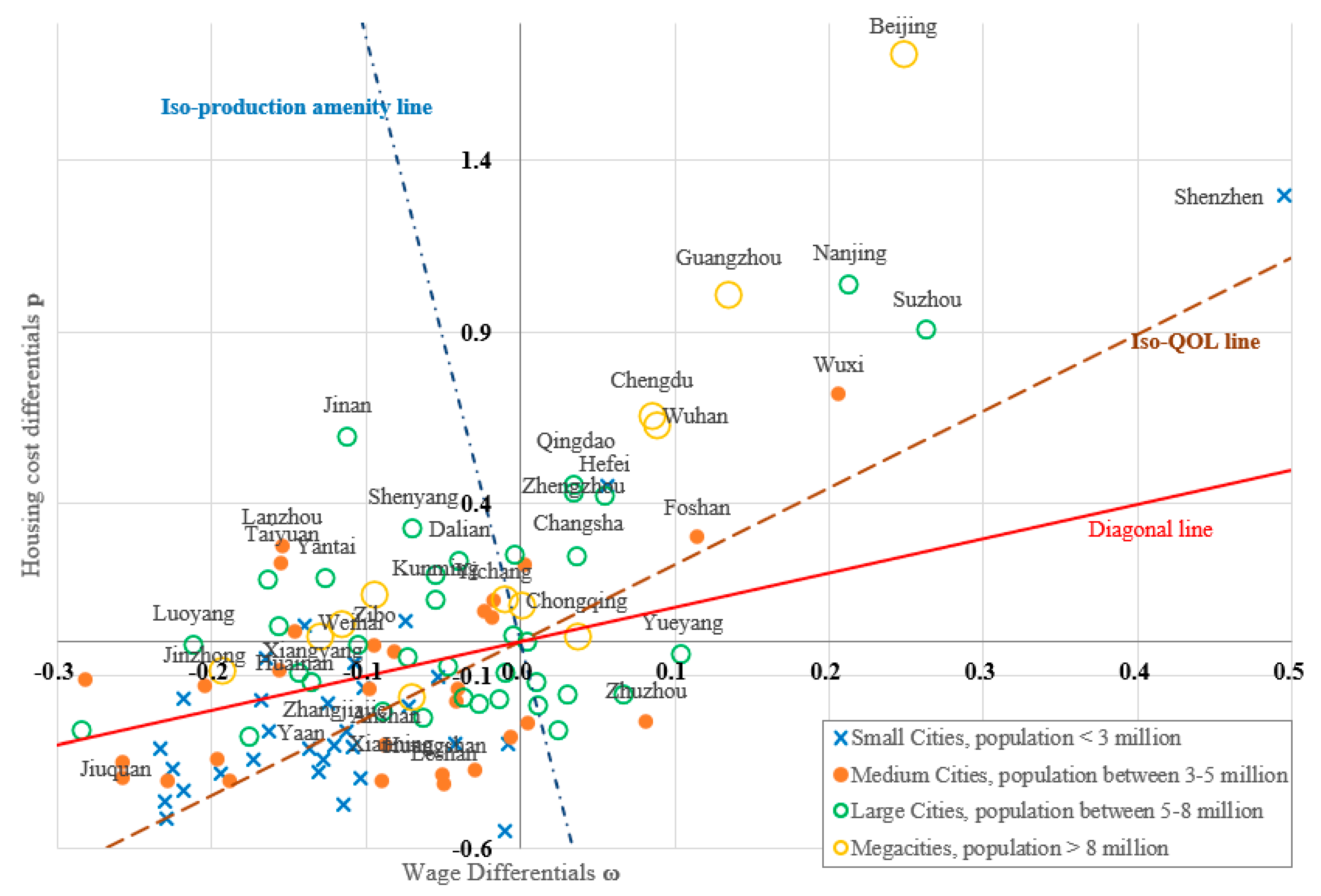
| Main Cities | Observed Prices | City Attributes | City Description | ||||
|---|---|---|---|---|---|---|---|
| Wage | Housing Cost | Production Amenity | QOL | Aver. Population | ln(GDP) | Areas | |
| Beijing | 0.25 | 1.71 | 0.30 | 0.35 | 1288 | 19.00 | 16,411 |
| Shenzhen | 0.49 | 1.30 | 0.50 | 0.06 | 278 | 18.68 | 1997 |
| Nanjing | 0.21 | 1.04 | 0.24 | 0.17 | 637 | 18.09 | 6587 |
| Guangzhou | 0.13 | 1.01 | 0.17 | 0.21 | 818 | 18.72 | 7434 |
| Suzhou | 0.26 | 0.90 | 0.28 | 0.09 | 645 | 18.60 | 8488 |
| Chengdu | 0.09 | 0.66 | 0.11 | 0.14 | 1168 | 18.21 | 12,121 |
| Jinan | −0.11 | 0.59 | −0.07 | 0.25 | 608 | 17.69 | 8177 |
| Wuhan | 0.09 | 0.63 | 0.11 | 0.13 | 825 | 18.20 | 8494 |
| Qingdao | 0.04 | 0.45 | 0.05 | 0.11 | 768 | 18.11 | 11,282 |
| Zhengzhou | 0.04 | 0.43 | 0.05 | 0.11 | 763 | 17.83 | 7446 |
| Hefei | 0.05 | 0.42 | 0.07 | 0.09 | 708 | 17.54 | 11,445 |
| Shenyang | −0.07 | 0.33 | −0.04 | 0.14 | 724 | 18.01 | 12,980 |
| Lanzhou | −0.15 | 0.28 | −0.12 | 0.19 | 322 | 16.57 | 13,086 |
| Taiyuan | −0.15 | 0.23 | −0.12 | 0.17 | 365 | 16.96 | 6977 |
| Changsha | 0.04 | 0.25 | 0.05 | 0.05 | 659 | 17.97 | 11,816 |
| Dalian | −0.04 | 0.23 | −0.02 | 0.10 | 589 | 18.06 | 12,574 |
| Kunming | −0.05 | 0.12 | −0.04 | 0.07 | 544 | 17.22 | 21,012 |
| Chongqing | 0.04 | 0.01 | 0.03 | −0.02 | 3337 | 18.55 | 82,374 |
| The average by population 1 | Obs. | ||||||
| Small Cities | −0.11 | −0.21 | −0.11 | 0.01 | 206 | 15.87 | 32 |
| Medium Cities | −0.08 | −0.11 | −0.08 | 0.02 | 381 | 16.48 | 30 |
| Large Cities | −0.04 | 0.07 | −0.03 | 0.05 | 635 | 16.97 | 37 |
| Megacities | 0 | 0.35 | 0.02 | 0.11 | 1180 | 17.61 | 12 |
| The average by GDP 2 | |||||||
| Underdeveloped Areas | −0.14 | −0.26 | −0.13 | 0.01 | 304 | 15.62 | 34 |
| Developing Areas | −0.08 | −0.17 | −0.08 | 0.00 | 482 | 16.40 | 38 |
| Developed Areas | 0.01 | 0.32 | 0.03 | 0.09 | 693 | 17.62 | 39 |
| Correlation | Obs. | |||
|---|---|---|---|---|
| 1 | 0.9571 | 111 | ||
| 2 | 2005 China Urban Quality of Life Report ① | 0.7043 | 0.6901 | 47 |
| 3 | Comprehensive Analysis of the Quality of Life in 287 Cities in 2006 ② | 0.6023 | 0.5689 | 111 |
| 4 | 2013 Chinese Urban Competitiveness Blue Book ③ | 0.6005 | 0.4576 | 111 |
| 5 | 2019 Top 100 Cities in China ④ | 0.7668 | 0.6348 | 49 |
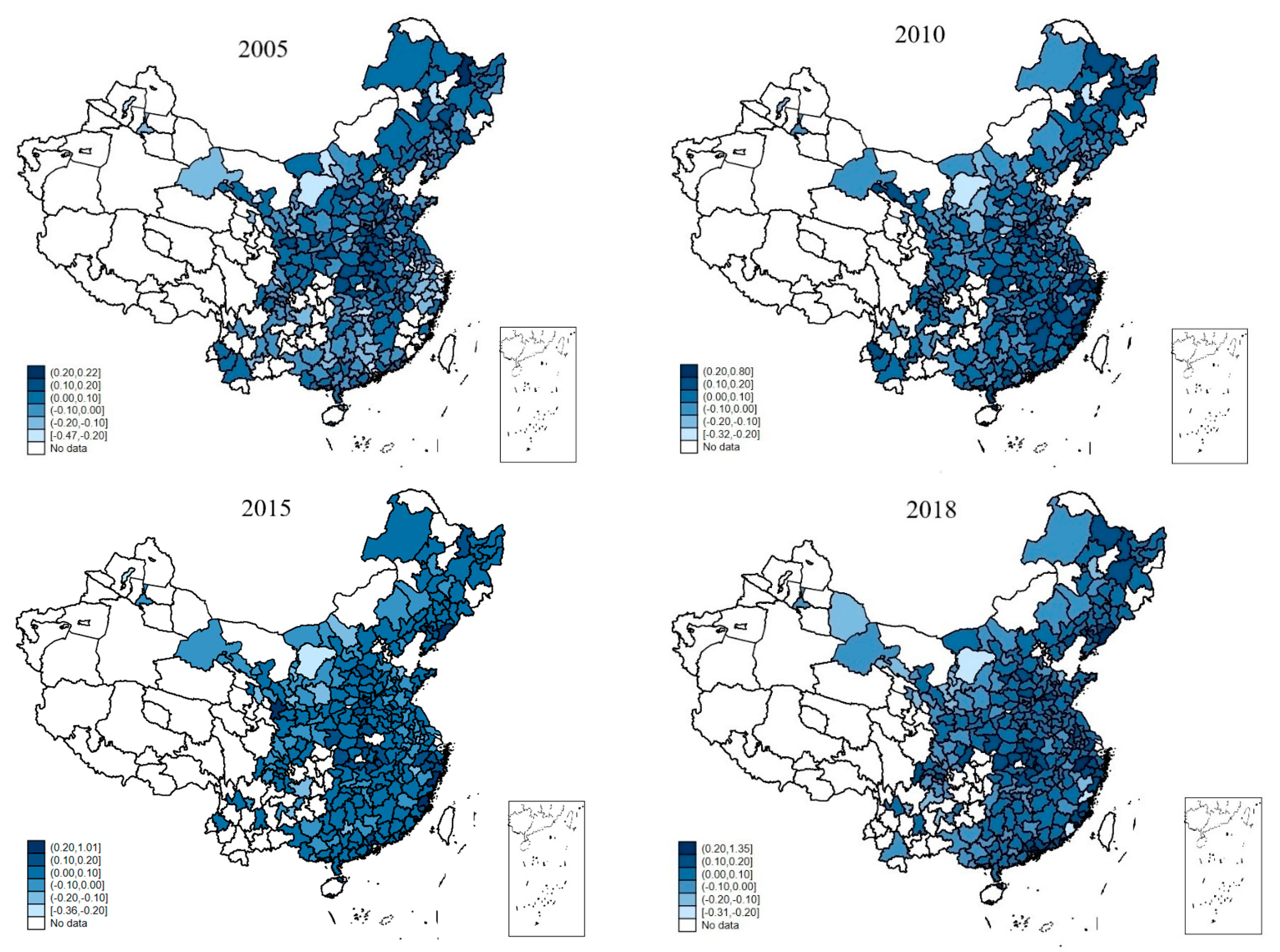
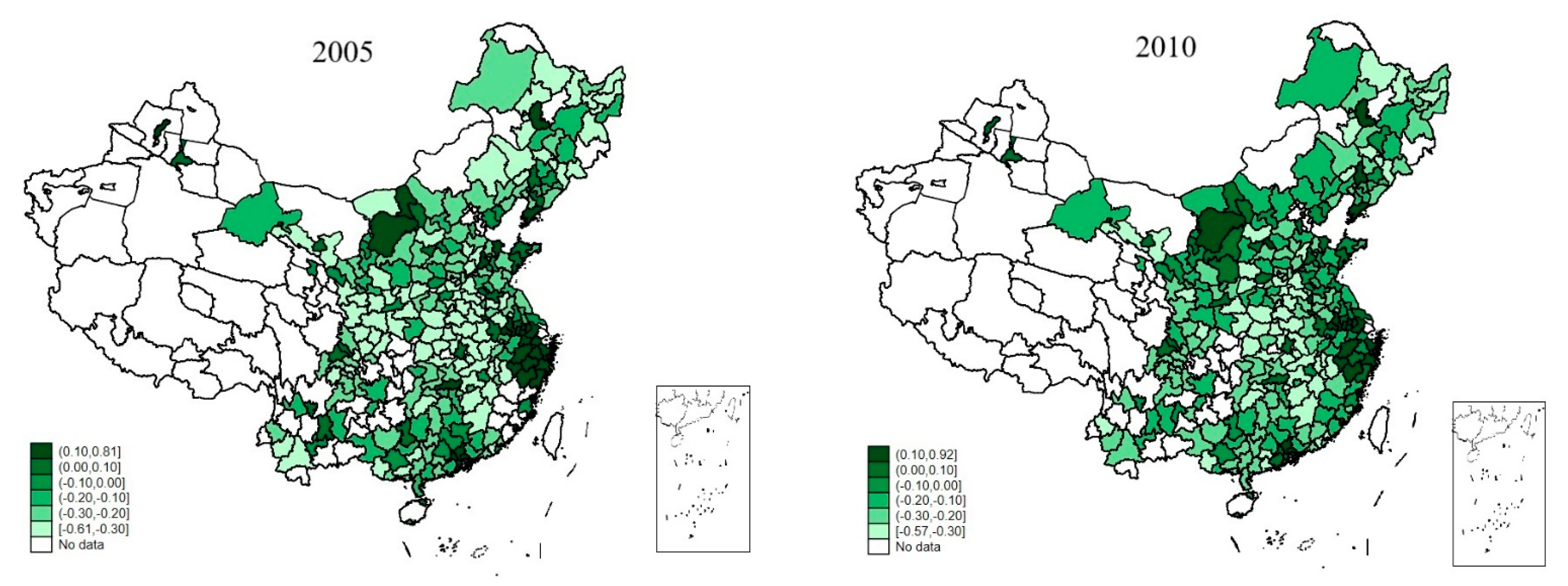
| 2005 | 2010 | 2015 | 2018 | 2005 | 2010 | 2015 | 2018 | |
|---|---|---|---|---|---|---|---|---|
| Mean | −0.024 | 0.030 | 0.033 | 0.045 | −0.157 | −0.151 | −0.143 | −0.151 |
| Obs. ① | 277 | 281 | 281 | 281 | 277 | 281 | 281 | 281 |
| # Positive Obs. | 134 | 182 | 197 | 204 | 54 | 55 | 42 | 39 |
| Max. | 0.217 | 0.799 | 1.011 | 1.348 | 0.813 | 0.916 | 0.810 | 0.820 |
| Min. | −0.471 | −0.319 | −0.362 | −0.315 | −0.609 | −0.574 | −0.835 | −0.472 |
| Top 5 | Yichun Zhoukou Sanya Heze Xinzhou | Sanya Shenzhen Wenzhou Zhuhai Hangzhou | Shenzhen Sanya Dingxi Xiamen Zhuhai | Shenzhen Sanya Zhuhai Xiamen Dongguan | Beijing Guangzhou Shenzhen Shanghai Hangzhou | Shanghai Beijing Shenzhen Guangzhou Tianjin | Beijing Shanghai Shenzhen Tianjin Guangzhou | Beijing Shanghai Shenzhen Guangzhou Nanjing |
| Urban Features | ||||||||
|---|---|---|---|---|---|---|---|---|
| Full-Samples | Sub-Sample by Population Size | Full-Samples | Sub-Sample by Population Size | |||||
| Large Cities | Small or Medium Cities | Large Cities | Small or Medium Cities | |||||
| (1) | (2) | (3) | (4) | (5) | (6) | |||
| Natural Features | Average annual temperature | X1 | 0.045 *** | 0.042 | 0.063 *** | 0.02 | 0.048 | 0.008 |
| (0.014) | (0.037) | (0.016) | (0.019) | (0.03) | (0.018) | |||
| Sunshine duration | X2 | 0.19 *** | 0.165 * | 0.152 * | −0.181 ** | −0.163 ** | −0.27 * | |
| (0.049) | (0.084) | (0.077) | (0.069) | (0.077) | (0.133) | |||
| Precipitation rate | X3 | −0.087 *** | −0.079 *** | −0.106 *** | 0.073 *** | 0.064 *** | 0.071 ** | |
| (0.013) | (0.019) | (0.022) | (0.018) | (0.021) | (0.034) | |||
| Social Features | Bus numbers | X4 | −0.011 | −0.003 | −0.023 ** | 0.031 *** | 0.035 *** | 0.044 *** |
| (0.007) | (0.011) | (0.009) | (0.011) | (0.012) | (0.016) | |||
| Mobile phones numbers | X6 | 0.017 * | −0.013 | 0.017 | 0.03 ** | 0.035 | 0.026 | |
| (0.01) | (0.015) | (0.012) | (0.013) | (0.022) | (0.021) | |||
| Water penetration rate | X8 | 0.149 *** | 0.088 * | 0.249 *** | 0.015 | 0.148 ** | 0.053 | |
| (0.036) | (0.048) | (0.08) | (0.058) | (0.07) | (0.105) | |||
| Drainage pipe density | X10 | 0.002 | −0.037 ** | 0.008 | 0.039 *** | 0.064 *** | 0.041 *** | |
| (0.007) | (0.015) | (0.008) | (0.009) | (0.019) | (0.014) | |||
| Green space per capita | X11 | 0.073 *** | 0.089 *** | 0.056 *** | −0.031 * | −0.046 * | −0.027 | |
| (0.013) | (0.019) | (0.018) | (0.018) | (0.026) | (0.023) | |||
| Wastewater discharge rate | X13 | −0.003 | −0.01 | −0.011 * | 0.012 ** | 0.041 *** | 0.013 | |
| (0.005) | (0.013) | (0.006) | (0.006) | (0.012) | (0.008) | |||
| Sewage treatment rate | X15 | 0.113 *** | 0.149 *** | 0.122 *** | −0.119 *** | −0.177 *** | −0.099 *** | |
| (0.013) | (0.03) | (0.017) | (0.021) | (0.044) | (0.021) | |||
| Population density | X18 | 0.021 *** | 0.051 *** | 0.023 *** | −0.012 | −0.023 | −0.015 | |
| (0.006) | (0.013) | (0.008) | (0.008) | (0.017) | (0.013) | |||
| Employment rate | X19 | −0.031 | 0.165 *** | −0.026 | 0.172 *** | 0.216 *** | 0.156 *** | |
| (0.027) | (0.033) | (0.018) | (0.02) | (0.048) | (0.023) | |||
| Cultural Features | Cinema numbers | X21 | 0.011 ** | 0.024 *** | 0.016 ** | 0.02 *** | 0.028 ** | 0.009 |
| (0.005) | (0.006) | (0.006) | (0.005) | (0.011) | (0.007) | |||
| Library collections | X22 | 0.022 *** | 0.026 * | 0.001 | 0.003 | −0.02 * | 0.008 | |
| (0.008) | (0.014) | (0.012) | (0.008) | (0.011) | (0.015) | |||
| Hospital Health Center numbers | X23 | 0.001 | 0.034 | −0.01 | −0.018 * | −0.068 ** | −0.014 | |
| (0.007) | (0.021) | (0.008) | (0.011) | (0.025) | (0.013) | |||
| Doctor numbers | X25 | 0.021 | −0.01 | 0.035 * | −0.056 *** | −0.027 | −0.057 ** | |
| (0.015) | (0.018) | (0.018) | (0.016) | (0.025) | (0.027) | |||
| College teacher numbers | X27 | 0.019 *** | −0.005 | 0.025 *** | 0.013 ** | 0.038 ** | 0.005 | |
| (0.004) | (0.01) | (0.005) | (0.006) | (0.014) | (0.006) | |||
| Proportion of employees in the tertiary industry | X28 | 0.111 *** | 0.091 *** | 0.13 *** | 0.004 | 0.039 | −0.029 | |
| (0.024) | (0.026) | (0.028) | (0.033) | (0.031) | (0.037) | |||
| R2 | 0.89 | 0.868 | 0.918 | 0.827 | 0.868 | 0.851 | ||
| Obs. | 111 | 49 | 62 | 111 | 49 | 52 | ||
Publisher’s Note: MDPI stays neutral with regard to jurisdictional claims in published maps and institutional affiliations. |
© 2022 by the authors. Licensee MDPI, Basel, Switzerland. This article is an open access article distributed under the terms and conditions of the Creative Commons Attribution (CC BY) license (https://creativecommons.org/licenses/by/4.0/).
Share and Cite
Zou, W.; Li, J.; Shu, Z. Urban Quality of Life and Production Amenity in Chinese Cities. Sustainability 2022, 14, 2434. https://doi.org/10.3390/su14042434
Zou W, Li J, Shu Z. Urban Quality of Life and Production Amenity in Chinese Cities. Sustainability. 2022; 14(4):2434. https://doi.org/10.3390/su14042434
Chicago/Turabian StyleZou, Wei, Jingjing Li, and Zhe Shu. 2022. "Urban Quality of Life and Production Amenity in Chinese Cities" Sustainability 14, no. 4: 2434. https://doi.org/10.3390/su14042434
APA StyleZou, W., Li, J., & Shu, Z. (2022). Urban Quality of Life and Production Amenity in Chinese Cities. Sustainability, 14(4), 2434. https://doi.org/10.3390/su14042434