Abstract
This paper deals with the optimization problem faced by the manufacturing engineering department of an international automotive company, concerning its supply chain design (i.e., decisions regarding which plants to open, how many components to produce, and the logistic flow from production to assembly plants). The intrinsic characteristics of the problem, such as stochasticity, the high number of products and components, and exogenous factors, make it complex to formulate and solve the mathematical models. Thus, new decision support systems integrating human choices and fast solution algorithms are needed. In this paper, we present an innovative and successful use case of such an approach, encompassing the decision-maker as an integral part of the optimization process. Moreover, the proposed approach allows the managers to conduct what-if analyses in real-time, taking robust decisions with respect to future scenarios, while shortening the time needed. As a byproduct, the proposed methodology requires neither the definition of a probability distribution nor the investigation of the user’s risk aversion.
1. Introduction
Enhancing efficiency, resilience, sustainability, and responsiveness in the supply chain is a relevant issue for automotive companies. Given the complexity of its products, this industry has a complex global supply chain. Indeed, it involves an intricate system of multiple actors engaged in various levels of collaboration (e.g., vehicle manufacturers, components suppliers, third-party contractors). Moreover, some information is not known a priori (e.g., product demand, travel times, duty costs, raw material price, political incentives). In this context, one of the biggest challenges faced by this industry is the design of a supply chain that guarantees customer satisfaction, considering the uncertainty of some parameters while containing the production costs. To better face this challenge, companies use the large amount of data they collect with powerful analytical tools [1,2]. Nevertheless, in order to make decisions, the results of statistical analysis are not enough. They must be integrated with the knowledge and insight of the decision-makers (such as tax constraints, marketing decisions, etc.), and properly defined optimization methods. This led to the need to redesign the existing decision support tools through a holistic vision of the system and, thus, a mix of qualitative and quantitative methods.
Several effective tools used for decision support rely on mathematical models that represent the problem. However, in a real setting, the resulting problem often becomes so complex that it cannot be solved due to the number of decision-makers involved (drivers, management, etc.), uncertainty, and exogenous constraints. Furthermore, since the decision environment is dynamic, some information can be revealed after decisions and new goals can be defined during the run (e.g., during economic crisis, the management takes more conservative decisions than in the normal period). These changes require frequent modifications in the mathematical model (e.g., adding constraints, considering new features, modifying the objective function), producing additional costs. This problem becomes even more impactful in stochastic problems, since the risk aversion of the decision maker must be taken into account, and several exogenous factors may impact the solution. It is worth noting that one possibility is to use multi-objective optimization ([3,4,5]). Nevertheless, its usage might be affected by the computational time needed and the tuning of different parameters, which is particularly needed when the number of objectives increase.
To overcome these issues, and to provide a general flexible framework, we define a Decision Support System (DSS) that is able to integrate choices dictated by the decision-maker, specific domain knowledge, and the potential of the DSS to optimally solve optimization problems. The main contribution of the present paper is the definition of a framework for integrating DSS and decision-makers in a more general framework.
In more detail, in this paper, we present a DSS developed by Politecnico di Torino (Turin, Italy) within a research project involving the Manufacturing Engineering department (ME) of the Italian automobile manufacturer Stellantis (formerly FCA) and World Class Manufacturing Research and Innovation team of Centro Ricerche Fiat (CRF). This DSS aims to support the ME managers in taking decisions concerning the production allocation problem and, thus, the optimization of component procurement activities for the different vehicle production (assembly) plants.
Through this DSS, the decision-makers can include their preferences in the development of a solution or a strategy and see how the performance is affected. For example, given the knowledge of the local labor force, the decision-maker may consider outsourcing a decision.
This is one of the several requirements that cannot be considered in the optimization model without increasing the model complexity outside the boundaries of computational tractability. A possibility when facing huge optimization problems encompassing several levels of decision is to split the main problem into several sub-problems (one for the tactical level, one for the operational one, etc.). Nevertheless, this yields several optimized subsystems, which are unable to correctly interact with each other.
In this context, this paper proposes the following main contributions:
- Design of a flexible and adaptable DSS supporting the managers in the automotive industry in making strategic production allocation decisions, integrating human choices and mathematical modeling in a stochastic environment.
- Formalize the strategic production allocation problem by a Mixed Integer Problem that considers both operational and managerial insight. We are particularly interested in the decisions about which plants to open, how many components to produce, and the logistic flow from production to assembly plants. Despite its simplicity, this model can encompass all the main characteristics of the Stellantis supply chain and be effectively solved to enable the decision-maker to take effective decisions also based on its knowledge and risk aversion.
- Present a managerial analysis of the strategic production allocation of the automotive industry. In doing so, we adopt a lean business approach named GUEST. Through practical tools, this method allows for an understanding of the business network, highlighting the interaction and needs of the different actors, as well as the value arising from the usage of a properly designed DSS to deal with their requirements [6,7].
It is worth noting that the proposed solution is currently used by ME managers to compute the solution satisfying most of their requirements and to conduct what-if analyses and, thus, investigate a set of scenarios within a reasonable time and consider the best possible solution. Moreover, this tool represents a means of assessing how the solution behaves in different settings and derive managerial insights. It is worth noting that the DSS presented in this paper has a general architecture that enables its usage in different contexts from the presented use-case.
The remainder of this paper is structured as follows. Section 2 reviews the literature on decision making under uncertainty. Section 3 describes the problem. Then, in Section 4, we present the GUEST methodology and how it has been implemented in our problem. In Section 5, we provide a managerial analysis of the complex system by using a lean management methodology. Then, Section 6 presents the mathematical model used to solve our problem. In Section 7 and Section 8, we present the architecture of the system and discuss the main results obtained by the adoption of the DSS in our industrial case study. Finally, we propose some conclusions and future research lines in Section 9.
2. Literature Review
Defining strategies and actions is a difficult task, especially when the decisions affect different functions and departments within the company. To solve this problem, companies usually use ad-hoc DSS. A broad literature exists on DSS, crossing arguments from different fields: decision science, information representation, Information Technology (IT) architecture, user behaviors, etc. For this reason, in this review, we focus on the literature about DSS, with an emphasis on the recent operation research applications using IT infrastructure.
Different optimization problems involve decision-making under uncertainty. This means choosing actions based on imperfect observations and information about the values of some parameters, resulting in unknown outcomes. The main mathematical tool to deal with this problem is optimization under uncertainty. This wide argument has been approached with different solution frameworks, including deterministic approximation [8], heuristic based on the problem structure [9,10]), exact method [11], and robust methods [12]. In the broad field of applications that involve stochastic optimization, we are interested in the supply chain. In this context, uncertainty affects several parameters, such as costs, demand, and supply. Moreover, unpredictable or unexpected events (e.g., terrorist attacks, earthquakes, and economic crises) may bring disruptive effects as business interruption. Indeed, although these kinds of disruptions usually have a low likelihood of occurrence, their impacts are prominent.
Optimization under uncertainty aims to achieve a configuration so that the supply chain can perform well under any possible realization of stochastic parameters. This topic has been faced by [13], who analyze different supply chain models considering uncertainty. Nevertheless, all the presented approaches consider few types of uncertainty and ignore that decision-makers’ preferences may change over time. This makes the model far less usable in real settings. It is also possible that changes in the environment (e.g., in the political setting of a country) may change the most important source of uncertainty and the risk aversion of the decision-maker over time. Solving these problems requires involving the decision-maker in the solution process. Thus, an ad-hoc DSS framework for dealing with the stochastic environment has to be developed [14]. In the literature, there are several examples of the successful application of these concepts [15,16,17].
It is worth noting that when organizations excessively rely on a DSS that does not involve the decision-maker, the outcome may be a wrong decision. This is particularly true when such tools are applied under high pressure and turbulent conditions. Furthermore, another source of error is that a DSS only has access to the company databases. This means that it lacks knowledge about exogenous factors such as law regulations, etc. For these reasons, the experience of the decision-maker is even more fundamental, as pointed out by the literature on the integration of humans and machines in Industry 4.0 [18,19].
These limits of the DSS have only recently been studied in the literature. Moreover, to our knowledge, there is no work dealing with DSS in the stochastic setting. Thus, the goal of this work is to fill that gap. In fact, DSS research primarily focuses on the technological aspects and design challenges [20,21] and only recently started to consider the organizational dimensions of strategic decision-making [22,23,24]. One of the first papers that consider DSS failure is the work by Aversa et al. [25]. In this paper, the authors study an iconic case of strategic failure in Formula 1 racing and propose an approach that integrates the decision-maker as well as the organizational and material context. Similar problems were also found in Wright et al. [26], Brauner et al. [27], and Althuizen et al. [28]. Despite the claims of these papers, related to the need to have a close interaction between the DSS and the decision-maker, no paper considers the problem in DSS modules dealing with the optimization of stochastic problems. By considering these suggestions, we design a new framework in which we treat the stochasticity using a simple mathematical model and the experience of the decision-maker. A similar approach has been considered in Jolly-Desodt and Jolly [29]. In this paper, the authors present a multi-criteria decision system that aims to help the operator of a human-machine system make suitable decisions about which tasks to execute at each moment. They use the framework of possibility theory [30], which allows a decision to be made based both on rules and preferences.
More recently, [31,32] propose a method called parametric cost function approximation. It uses deterministic problems modified through opportunely tuned parameters to approximate stochastic programming. Concerning this young branch of the literature, we integrate the decision maker in the modeling phase, by enabling him to perform the tuning of the parameters. It is worth noting that some iterative decision processes were already considered in the context of fuzzy systems [33]. Moreover, simulation-based approaches have been applied in the automotive supply chain [34]. Nevertheless, despite being similar in terms of goal, both [33,34] do not tackle stochastic problems directly. Thus, their implementation is very distant from our approach.
3. Problem Description
In this paper, we consider the ME manager of an international automotive company that deals with the production allocation problem. The manager copes with the optimization of procurement activities and, thus, the supply of components from the production plans to the different vehicles’ assembly sites. In particular, the decisions that we consider are: (i) the selection of which plant to open, i.e., the plant in which the production will be active, (ii) the choice of the production step to activate in each active plant, (iii) the logistic flow from the production to the assembly plants. Making these decisions requires considering the market forecasting analysis concerning the future vehicles’ demand in the different countries in which the company is located.
Without loss of generality, we suppose that each assembly plant produces one type of vehicle that requires certain semi-finished products and components. Thus, the ME manager aims to determine a procurement and allocation plan, identifying what quantity of these components should be procured from each supplier to satisfy the estimated demand in each assembly plant.
In doing so, the ME manager aims to minimize the total cost of the procurement plan, which includes the manufacturing and transportation costs, while avoiding inventory overstocks in the warehouses.
The ME manager has the following information:
- The production steps that correspond to the combination of the volumes of the different components that the plant can produce;
- The investments used to open a new plant with a specific production step;
- The Product Value Added (PVA), which is the added actual value corresponding to the unit costs for each component type produced in a specific production step;
- The outbound logistics costs, which are the unit costs for the transport of components among plants;
- The duties expressed as a percentage of the total cost;
- The inbound logistics costs, corresponding to the unit cost to transport the component within the country where the plant is located;
- The Direct Material Cost (DMC), that is, the unit costs for the production of items;
- The markup cost is the ratio between the production cost and the final selling price.
This information is subject to variability due to price variations in raw materials, the incentives of the countries involved in the process, environmental laws, sudden changes in duty cost (e.g., commercial wars between states), and many other factors. Moreover, the different sources of uncertainty may have different impacts over time. For example, sudden changes in duty cost can be more likely depending on the governments of the states. Of course, no model actively considers all these sources of uncertainty, since this would result in too complex an optimization model. Finally, operating in a real setting means dealing with a dynamic environment. This makes obtaining a precise definition of the problem a priori difficult, given the number of changing parameters. For example, a sudden change in the cross-border taxes may require considering that aspect in the models, while before this was not an issue. Thus, the decision maker has to be involved in the modeling phase.
4. Methodology
As introduced in Section 1, we adopted the GUEST methodology, developed by a pool of researchers of Politecnico di Torino [6,7]. The GUEST method has been applied to more than 50 companies and 20 innovation projects to date, including projects with up to 30 partners. It is a lean business methodology extending the work by the Lean Startup movement, which provides a scientific approach to developing products and solutions faster, shortening the development process. The GUEST adapts its results to the environment of a Multi-Actor Complex System (MACS), such as the automotive industry. In this industry, the complexity is increasing due to the presence of several actors with different areas of expertise (manufacturing engineers, assemblers, etc.) that interact and pursue their (sometimes conflicting) objectives and goals, as well as the evolving customer needs and environmental concerns.
The GUEST is an easy-to-understand methodology, which is applicable to the entire decision-making process to increase efficiency and improve quality for the companies. It controls the process, from the original idea to its implementation, providing conceptual and practical tools to the different actors involved, enabling them to communicate their vision, difficulties, and opportunities within the same structure. This contributes to reducing the time needed to implement their decisions in the system, and the general development time of the model, from the beginning of the project to the definition and validation of the model and evaluation of the outcomes [2,35,36,37]. For these reasons, we selected the GUEST method, as it represents a powerful methodology in our use case. GUEST is articulated in five steps (i.e., Go, Uniform, Evaluate, Solve, and Test), and each step allows the actors to monitor their projects and, at the same time, standardizes the documents and tools that should be used to evaluate ideas, successes, actions, and results. The five phases of the methodology are:
- Go: this aims to provide a full description of the stakeholder profile, its current behavior, its environment, the external actors in the system, and their interactions.
- Uniform: as the name suggests, this phase aims to standardize the knowledge and information collected in the Go phase. The governance and business models are explicitly described.
- Evaluate: the governance and the business model are assessed in a series of actions.
- Solve: given the specific problems and the actions highlighted to cope with them, a list of operational models is proposed.
- Test: the actions are implemented and their performance evaluated.
For more details about these five steps, the interested reader can refer to the manifesto [6].
5. Managerial Analysis
In this section, we apply the GUEST methodology to identify and describe the actors involved, with an emphasis on their requirements [6,7].
We first define the actors and the value proposition that a DSS could offer to them (Section 5.1). Then, we depict the solution canvas (Section 5.2).
5.1. Actors
The first step is to define the actors involved in the process and their profiles. In doing so, according to the principles of the Value Ring [6,7] and Value Proposition Canvas [38], we break the actors’ profile down into different factors related to their jobs (i.e., what they are trying to achieve in their work), pains (i.e., problems, risks, and obstacles related to their jobs), and gains (i.e., what they are trying to achieve in their work). Then, we prioritize these jobs, gains, and pains, highlighting the most important or urgent ones that must be considered in our solution.
Our production allocation problem considers the following three key players:
- Manager of the Manufacturing Engineering department (ME) at the global level. Marketing experts provide the ME manager the estimation of the demand for vehicles in each region. The ME manager seeks to secure adequate volumes of components from the component plants that satisfy the demand of vehicles at the minimum cost, avoiding oversupply.
- Manager of the Components Plants (CP), who represents the supplier of the components.
- Manager of the vehicle assembly plants, named Vehicles Plants (VP). This is in charge of assembly operations to produce cars and commercial vehicles.
Figure 1 shows the Value Ring and depicts the value proposition that the adoption of DSS could offer to the above-listed actors. In particular, the width of the angular area of the value ring associated with each actor represents its importance. Each color describes the priority of each gain-creator or pain-reliever (i.e., red, yellow, and green are high, medium, and low priorities, respectively).
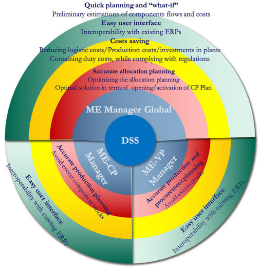
Figure 1.
Value Ring.
The first actor who plays a central role in our use case is the ME Manager Global. As discussed, according to the expected forecast of vehicle demand, the ME Manager Global determines an accurate procurement and allocation plan. This particularly concerns the optimal quantity of components to procure from each supplier and allocate in each assembly plant to fulfill the market demand of vehicles. An assembly plant is responsible for the production of a specific type of vehicle, which requires certain components (e.g., car doors, bumper). Thus, the DSS provides the ME Manager Global with a tool to optimize the activation/opening strategy of CP plants.
From a medium-term perspective, one of the most critical issues that the ME Manager Global has to face is the optimization of the costs. This means that the manager has to implement an optimal plan in terms of the selection of plants to activate and the volume of components to procure in each plant, which contains the overall costs. We consider three types of expenses: (i) investment to activate CP plants with a certain production step (in terms of different types of component that can be produced); (ii) production costs; (iii) transportation and logistics costs, related to the inbound and outbound activities; (iv) duty costs, which refer to the taxes paid in compliance with the regulation of each region, expressed as a percentage of the total components’ production and logistics costs.
Finally, in the long run, the ME Manager Global is interested in a handy and reactive tool that allows for planning activities to be conducted and what-if analyzed within a reasonable time. It has to provide a preliminary estimation of component flows and related costs before the detailed production and destination planning. A user-friendly interface for the DSS and its interoperability with existing software play a relevant role in facilitating decision-making and information exchange among ME, CP and VP managers, as well as the board of directors.
Using the proposed DSS, the CP and VP managers benefit from accurate production planning. Indeed, a CP manager could plan the optimal production level of a certain component. Similarly, the proposed tool supports the VP manager in the definition of the production plan and in supporting the procurement activity, defining the optimal quantity of components to buy from CPs. The optimized production planning in CPs and VPs mitigates the risks of oversupplying, reducing the excess of component/vehicle stocks in the warehouses along the supply chain.
Finally, as the ME Manager Global, the CP and VP managers are also interested in a user-friendly and interoperable tool.
5.2. Solution Canvas
This section analyzes the Solution Canvas (Figure 2) designed for our case study. The solution canvas is an analytical tool used in the GUEST methodology to outline the chosen solution and apply and address the needs and requirements that emerged in the actor analysis.
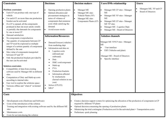
Figure 2.
Solution Canvas.
The remaining part of this section is devoted to going through the details of each building block that comprises the canvas.
The decision-makers are represented by the ME Manager Global, CP Manager, and VP Manager taking the decisions concerning the activation of plants and the production and procurement planning, as discussed in Section 5.1. Moreover, the ME Manager Global should foster and promote the adoption of the proposed technology.
The users of the DSS-based solution are the actors presented in the previous subsection and also the Board of Directors of the company, who would like to receive the DSS, summary data, and information about costs.
Regarding the relationships between the decision-makers and the users, the CP Manager interacts with the ME Manager Global to obtain detailed information, optimizing and planning the inbound flows of components. Similarly, the ME Manager Global interacts with the VP Manager to obtain detailed information concerning the production of vehicles, optimizing, and planning the procurement of components and the overall production. CP and VP Managers interact to book the time slot, and deliver the components to the vehicles’ production plants. This activity also requires interaction between ME Manager Global and the Logistics department of the company. Finally, the ME Manager Global interacts with the Board of Directors to ensure and report a timely and relevant information flow (e.g., costs, production levels).
The main channel through which the solution could be implemented, allowing the outcome to be obtained and reported for each identified relationship, is the user interface of the solver.
The objectives of the proposed solution are:
- Create a DSS to optimize the allocation of the production of CP components required by different VP plants;
- Take the optimal decision concerning the opening of production plants;
- Minimize the total cost per engine, including the transportation and production costs;
- Obtain a preliminary quick planning, postponing the details to a subsequent phase.
The main decisions are related to the key elements of the solution and the requirements that emerged in the actor analysis. In particular, the decisions regard:
- The opening of production/components plants;
- The design and deployment of optimal allocation and procurement strategies in terms of volumes of components that minimize costs, while satisfying the demand;
- The reduction in excess stocks of components and vehicles.
To implement this solution, the principal resource needed is the mixed-integer linear programming (MILP) model. Another relevant resource concerns the Gurobi Optimizer software needed to solve this [39]. Moreover, the principal information needed to be input to the solver is the estimation of vehicle demand by marketing research and other information mentioned in Section 3 (i.e., production steps, amount of investments needed to open a new plant, PVA, outbound/inbound logistics costs, duties, DMC and markup).
The solution implies some constraints that must be considered in the implementation phase. They can be classified into problem and solution constraints. The former refers to the constraints included in the MILP model, as described in Section 6. The latter can be summarized as follows:
- Compatibility of data from existing enterprise resource planning software (ERP) used by Manager ME in the different sites;
- Computation of duties and mark-up costs according to internal rules;
- Easy tool to explore the solution space;
- Availability of an offline version and ability to produce a what-if analysis within a reasonable time.
Finally, the last building block of the solution canvas concerns the costs of the solution. They can be grouped into four main categories:
- Development costs that are related to the implementation of the solver. They refer, for example, to the expenditure for hardware and software assets, such as the Gurobi license.
- Cost of the introduction of the solution. This refers to the training costs of all the managers and the integration of a solution with the current ERPs and company systems.
- Maintenance costs. As the term suggests, these refer to the cost of maintaining the whole infrastructure and guaranteeing its correct functioning.
- Cost of not introducing the solution. This refers to all the inefficiencies along the supply chain that determine additional economic efforts (e.g., the cost of excess stocks and time spent in inefficient planning activity).
6. Mathematical Model
This section presents the mathematical model formulated to address the described problem. It considers the following sets:
- is the set of the production plants;
- is the set of engines;
- , is the set of production steps for each production plant and each engine type we consider;
- is the set of destination sites;
- is the set of the final product.
The parameters used are as follows:
- is the cost of activating the production of the engines considered in plant ;
- is the maximum number of engines that can be produced in plant if production step has been activated;
- is the number of engine needed for the final item ;
- is the cost of activation of production step for engine and plant ;
- is the PVA costs paid by plant to produce the engine if step is activated;
- is the amortization cost paid by plant to produce the engine if step is activated;
- is the DMC cost paid by plant to produce the engine if step is activated;
- represents the markup cost paid by plant to produce the engine if step is activated;
- is the unitary logistic cost of moving engine from production plant to destination plant .
- is the demand of product p in destination site j.
Finally, the decision variables are:
- is equal to 1 if the production plant is open, and 0 otherwise;
- is the quantity of engine produced in plant using production steps ;
- is equal to 1 if the production steps is activate in order to produce engine in plant , and 0 otherwise;
- is the quantity of engine shipped from production plant to destination plant ;
- is the quantity of engine shipped from production plant and shipped to destination plant if the production steps is activate;
- is the quantity of engine in destination plant ;
- is the quantity of final product assembled in destination plant .
The model can be expressed as follows:
subject to:
The objective function (1) minimizes the total cost related to the opening of production plants, and production and transportation costs. The first term is related to the activation costs, the second term accounts for PVA costs, the third quantifies depreciation costs, the fourth considers the markup costs, and the last term accounts for logistic costs.
Constraints (2) link the variable y and the variables v, while constraints (3) link the variable v to the variable x. Constraint (4) limits the number of out-coming products to the one produced. Constraints (5) and (6) link the variable u to the variables w and x, respectively. Instead, constraints (8) define the production of the final product and (9) impose that the demand of the final products must be satisfied. Finally, constraints (10) describe the domain for each decision variable.
Despite its simplicity, the model can consider all the main decisions that the company has to take and the sources of uncertainty in its supply chain. It is worth noting that the main innovation of the paper is the general framework for the model formulation (i.e., the GUEST methodology) and the solution method that, instead of solving a complex model encompassing all possible sources of uncertainty, directly involves the decision-maker as an active part of the solution choice process.
Alternative Scenarios Generation
Since the DSS allows the ME to compare how the different solutions behave in different scenarios, we define an ad-hoc procedure that enables the user to dynamically change and adapt the scenarios in the run. In particular, given a solution to the problem (1)–(10), in a certain scenario that occurs with probability , we split the different levels of choice, i.e., which plant to open y, the opening level of each plant z and the final logistic decisions w. Thus, for each scenario, we define its best solution and the respective variable: .
Starting from the first level of decision (e.g., which plant to open) and considering the probability of all scenarios to be identical, we define the coverage of the solution as the percentage of scenarios in which is the best solution, i.e.,
where is the cardinally operator, i.e., the number of items in the set. The operator can be generalized to z and w. Nevertheless, since the variables z depend on the variables y and the variables w depend on z and y, we consider the coverage of z and w conditioned by the upper-level solution, i.e., and . Their meaning can be expressed as follows:
7. IT Architecture
In this section, we present the architecture of the system infrastructure, as shown in Figure 3. The DSS is organized into four main components: web interface, computation unit, exact solver and Data Bases (DBs) (intuitively divided in Solution DB, Instance DB and User DB).
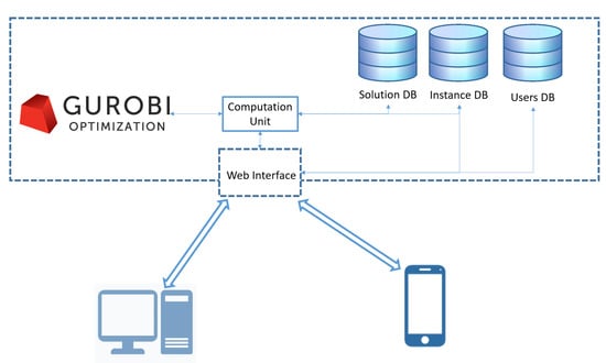
Figure 3.
System architecture of the DSS.
The first step to access the platform is the creation of an account in Users DB. Registered users have access to a web interface that, after a log-in phase, gives them three possibilities: (i) insert one instance; (ii) explore the set of instances that were previously inserted; (iii) navigate the set of solutions. It is worth noting that the platform offers the possibility of managing the visibility of the instances, as well as the solution for different users.
Figure 4 depicts a part of the page for instance insertion. This page is devoted to data collection and saves the information in Instance DB.

Figure 4.
Example of form for inserting instance data.
In particular, the system required the duty costs, engine demands, logistic costs, and material costs of three possible values associated with a positive scenario, a negative and an average one. In our example, the positive and negative scenarios are changes of in the average parameters.
Once all data are inserted, the system adds two other scenarios: one between the positive and the average and one between the average and the negative. Thus, problems are solved in parallel to provide the initial set of solutions. Since having more solutions for the same instance can provide more alternatives for the users, we use the Solution Pool method provided by Gurobi. This step takes around 5 min and the new solutions are stored in Solution DB a non-relational database implemented in Mongo DB. The choice of this technology has been effective in querying the solution set and computing the indicators in Equations (11)–(13). In fact, by using not relational databases, it is possible to store the solutions as they are produced by the solver and then make queries in a easy and effective way.
Each user can see the instances inserted through synoptic representations, which are not reported because they are beyond the scope of the paper.
In the following, we present the core of the solution navigation part. This is the core of the DSS that was developed by a strict collaboration with the Stellantis management. The principle is to divide the various levels of the solution: facility location, level of activation, and logistic choices in different pages. We consider two pages: one representing the facility location and activation level (Figure 5), and one representing the corresponding logistic flows (Figure 6). We illustrate the main part of the DSS by considering a small instance with 4 production plants, 4 destination plants, and 4 types of engines.
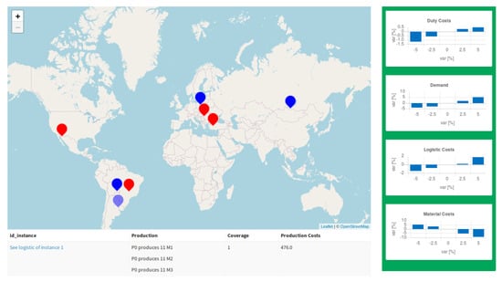
Figure 5.
Location analysis.
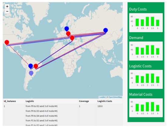
Figure 6.
Logistic analysis.
On the first page, shown in Figure 5, the user sees which facility must be open on a map. The table below the map shows the possible choices of the level of productions for each open plant. In particular, the first column shows the identification of the solution (if clicked once, it selects the instance, while if clicked two times, it links to the corresponding logistic page), the second column describes the production level for each engine in each plant, the third one describes the coverage in (11) and the associated cost.
The graphs on the right part of the page show how the costs of the selected solution change in the range of possible variations in the parameters. In the example, the decision-maker can observe that the impact of a variation in duty cost is greater than demand variations, which are greater than logistic costs.
Even if this representation does not provide an analysis of the variations in more than one parameter, its realization was strongly suggested by the end-user and it has been used extensively by the management.
By selecting the solution identification name, a set of modal windows will appear, allowing the user to insert new scenarios. Once that the inserting phase is finished, in a few seconds, the system shows the performance of the solution in the new scenarios, updates the graphs and stores the optimal solutions relative to the new scenarios in the DB. By double-clicking on the name of the instance, the user is redirected to the page presenting the logistic solution (see Figure 6).
This page is organized similarly to the previous one. In the map, the logistic flows are represented by straight lines from the origin to the destination; the different colors represent the different type of engines. By clicking on each line, it is possible to obtain details related to the origin, destination, type, and quantity of the shipped engines. As in the previous page, the table below the map shows the solution identification name, the logistics dtails, the coverage rate, and the logistic costs of the solution. Furthermore, the graphs on the right have the same meaning as the ones on the previous page. The ones shown in Figure 6 are randomly generated because they are more sensitive for the company. As in the previous page, it is possible to add a new instance by right-clicking on the name of the instance.
8. Numerical Experiments
In this section, we conduct an experimental campaign with the following objectives:
- Measure the performance of the proposed solution method;
- Demonstrate how this DSS supports the managers in taking decisions in a reasonable time;
- Assess the impact of the problem parameters on the production allocation.
It is worth noting that, by using the proposed approach, the decision-maker can very quickly make decisions. In fact, for the usual decision stream required from the top management to propose solutions that the other sectors of the company have to evaluate, this produces several iterations that last for days. Instead, by using the proposed methodology, the top management can reduce this time to few seconds. This is one of the features of the proposed DSS that is most appreciated by the company.
In the following subsections, we present the instance sets used to qualify our model and the solution procedure (Section 8.1), and we discuss the computational results in Section 8.2.
8.1. Instances
In this section, we describe the method used to generate the set of instances used for the numerical experiments. The parameters used for the instance generation were defined in agreement with the practices adopted by the company. However, for privacy reasons, we have not presented real data, only the parameters used to generate a realistic scenario. These parameters are as follows:
- The number of production plants I has been considered in the set 3–5.
- The number of different engines M produced in the production plants has been considered in the set 3–5.
- The number of production steps for each production plants and each engine type is in the range 3–4.
- The number of destination sites J is in the range 3–5.
- We consider the production of a single final product P.
- The cost for activate the production of the considered engines in plant is assumed equals to 100 million
- The maximum number of engines that can be produced in plant if production step has been activated ranges between .
- Each vehicle P require a single engine, thus is equal to one;
- The cost of activation of production step is assumed to be equal to 5,000,000 k.
- The PVA and the DMC costs have been generated by using normal distribution with parameters and , respectively.
- The amortization cost is computed as .
- A markup is set equal to the 15% of the DMC cost.
- The unitary logistic cost for moving engines among the production and destination plants is equal to .
- Finally, the demand of product is in the range (100,000; 20,000).
A summary of these values is presented in Table 1.

Table 1.
Distribution of the parameters for instance generation.
It is worth noting that these data are quite general and describe the settings of a general car-maker company.
8.2. Results
As previously mentioned, the proposed DSS allows the managers to conduct what-if analyses in real-time. Thus, we present the computational time needed to solve model (1)–(10) for instances characterised by different dimensions in Table 2 (all the results are obtained by averaging 100 instances).
Table 2.
Solution time and standard deviations for different instance dimension.
Despite the increase in complexity, all the instances were solved in less than 1 second. Since our goal is not only to compute the optimal solution but to obtain a set of good solutions, we use the PoolSolutions function of Gurobi and set the PoolSolutions parameter to be equal to 10, i.e., the ten best solutions are computed and returned. As expected, the computation time increases as the dimension of the instance increases. Furthermore, the parameter that most affects the complexity of the model is the number of production plants, I. This is reasonable since the greater the I, the more possibilities there are regarding which plant to open, which production step to activate, etc.
Usually, problems affected by stocasticity are solved by using apposite techniques such as robust programming, stochastic programming, etc. In order to compare our DSS with a standard solution method, we defined the following two-stage stochastic problem that generalizes model (1)–(10) to the stochastic setting.
subject to:
In model (17)–(24), the objective function considers the expected value of the costs. The parameter is a penalty term for lost sales and . It was added since the Constraints (9) in the stochastic settings can be difficult to satisfy. It worth noting that the last term in the objective function is not linear; therefore, it is necessary to linearize it by adding slack variables. Comparing the performance of the proposed methodology with that of the aforementioned stochastic program is a difficult task. In fact, the proposed approach may consider factors that are not described in the mathematical model. Furthermore, the proposed solution method needs a decision-maker to compare and analyze the deterministic solutions of model (1)–(10) in different scenarios. This last consideration must be highlighted since it is the way in which the proposed approach faces uncertainty, as well as the main difference between the proposed approach and the present literature. Due to this characteristic, we select a decision-maker to find the test solution of the test instance for a Stellantis manager. The final difficulty that we face when comparing the proposed methodology is that the out-of-sample stability of the two-stage model (17)–(24) reaches values below for a higher number of scenarios than an exact solver can handle. This makes it more difficult to make a direct comparison between the solutions of the stochastic model and the one provided by our approach. Thus, for the three y with the highest covering () obtained by the proposed methodology, we compute the second-stage value and compare them against the second-stage value of the expected values’ solution, i.e., the solution obtained by the stochastic model by replacing each random variable with its expected value. We are aware that this experiment is not a full proof of the effectiveness of the proposed method against the general solution of the two-stage problem. Nevertheless, it provides some feedback regarding the goodness of the solution that the decision-maker can take. It is worth noting that the only proof that the proposed methodologies are working derives from the ME using the DSS. The fact that the company is using this tool is, by itself, the needed proof.
We call the average activation cost () reduction obtained by using the solution with i-th highest covering instead of the expected value solution. We report the results in Table 3.
Table 3.
Average cost reductions.
The value of is always greater than the value of , which is greater than the value of . This is reasonable, since the covering definition is a measure of the extent to which solution y is robust with respect to uncertainty. It is interesting to note the magnitude of this trend. The average of the first column is , the average of the second is , and the average of the third is . This is due to the reduced number of first-stage solutions, in fact, given I production plants, the possible first-stage solutions are . Thus, in the considered instance, the number of first-stage solutions varies between 8 and 32. This, in combination with an objective function deeply influenced by the cost of opening a facility (these costs are the ones with the greatest impact), leads the problem to have few good solutions in the deterministic as well as in the stochastic settings. Furthermore, the gain that we obtain increases as the dimensions of the problem increase. This means that, by using our proposed approach, we exploit the information coming from the stochasticity of the problem. Since the instances are based on realistic data, these results are the main simulated proof of work that, together with the real usage of the software, enable us to prove the effectiveness of our method.
9. Conclusions
In this paper, we introduced a new paradigm for dealing with stochastic problems in the DSS domain. This paradigm was developed with the help of the top management of Stellantis, one of the leading companies in the automotive sector. The main weakness that our paradigm is addressing is the impossibility of a mathematical model that can consider all the characteristics of real-life scenarios (e.g., political constraints, sustainability and marketing choices). Furthermore, the proposed DSS gives the decision-maker the possibility of simulating, in real-time, what the behavior of a solution would be if a new scenario appears, thus providing a tool for real-time what-if analysis. Finally, this framework, by giving the decision-maker the possibility of inserting scenarios and choosing a solution to implement, does not require an a priori definition of the risk aversion of the users or the probability distribution of the scenarios. These aspects are the two main gaps in the stochastic literature, which requires an a priori choice of risk aversion and probability distribution for the model parameters. In conclusion, due to the good solutions that the approach can find, this paper paves the way to an approach to tackle uncertainty that, instead of relying on a complex model, involves the decision-maker in the solution method. Moreover, the presented application is the first evidence that the proposed methodology can be effectively used in practice. Despite being developed for the automotive industry, the same methodology can be used in all complex decision-making problems that are subject to uncertainty. Future work will study how to provide more effective interfaces between the user and the solution database, as well as applying this methodology to other case studies. Moreover, a promising future line of research consists of developing artificial intelligence techniques to mimic the decision process of the user, thus proposing better solutions.
Author Contributions
Conceptualization, G.P., E.F. and M.R.; methodology, G.P.; software, E.F.; validation, J.E.M. and D.M. All authors have read and agreed to the published version of the manuscript.
Funding
This research was funded by Stellantis in its Research Grant agreement with Politecnico di Torino.
Informed Consent Statement
Not applicable.
Conflicts of Interest
The authors declare no conflict of interest.
References
- Brotcorne, L.; Perboli, G.; Rosano, M.; Wei, Q. A Managerial Analysis of Urban Parcel Delivery: A Lean Business Approach. Sustainability 2019, 11, 3439. [Google Scholar] [CrossRef]
- Perboli, G.; Musso, S.; Rosano, M. Blockchain in Logistics and Supply Chain: A Lean Approach for Designing Real-World Use Cases. IEEE Access 2018, 6, 62018–62028. [Google Scholar] [CrossRef]
- Wang, C.N.; Nguyen, N.A.T.; Dang, T.T.; Lu, C.M. A Compromised Decision-Making Approach to Third-Party Logistics Selection in Sustainable Supply Chain Using Fuzzy AHP and Fuzzy VIKOR Methods. Mathematics 2021, 9, 886. [Google Scholar] [CrossRef]
- Nguyen, N.B.T.; Lin, G.H.; Dang, T.T. A Two Phase Integrated Fuzzy Decision-Making Framework for Green Supplier Selection in the Coffee Bean Supply Chain. Mathematics 2021, 9, 1923. [Google Scholar] [CrossRef]
- Ibrahim, N.; Cox, S.; Mills, R.; Aftelak, A.; Shah, H. Multi-objective decision-making methods for optimising CO2 decisions in the automotive industry. J. Clean. Prod. 2021, 314, 128037. [Google Scholar] [CrossRef]
- Perboli, G. The GUEST Methodology. 2017. Available online: https://staff.polito.it/guido.perboli/GUEST-site/docs/GUEST_Metodology_ENG.pdf (accessed on 15 February 2020).
- GUEST. The GUEST Initiative Web Site. 2017. Available online: http://www.theguestmethod.com (accessed on 15 February 2020).
- Kan, Y.S.; Vasil’eva, S.N. Deterministic Approximation of Stochastic Programming Problems with Probabilistic Constraints. In Mathematical Optimization Theory and Operations Research; Bykadorov, I., Strusevich, V., Tchemisova, T., Eds.; Springer International Publishing: Cham, Switzerland, 2019; pp. 497–507. [Google Scholar]
- Gaudioso, M.; Monaco, M.F.; Sammarra, M. A Lagrangian heuristics for the truck scheduling problem in multi-door, multi-product Cross-Docking with constant processing time. Omega 2020, 101, 102255. [Google Scholar] [CrossRef]
- Dempster, M.A.H.; Fisher, M.L.; Jansen, L.; Lageweg, B.J.; Lenstra, J.K.; Rinnooy Kan, A.H.G. Analysis of Heuristics for Stochastic Programming: Results for Hierarchical Scheduling Problems. Math. Oper. Res. 1983, 8, 525–537. [Google Scholar] [CrossRef][Green Version]
- Qin, Y.; Wang, R.; Vakharia, A.J.; Chen, Y.; Seref, M.M. The newsvendor problem: Review and directions for future research. Eur. J. Oper. Res. 2011, 213, 361–374. [Google Scholar] [CrossRef]
- Bishop, M.; Elliott, C. Robust Programming by Example. In Information Assurance and Security Education and Training; Dodge, R.C., Futcher, L., Eds.; Springer: Berlin/Heidelberg, Germany, 2013; pp. 140–147. [Google Scholar]
- Govindan, K.; Fattahi, M.; Keyvanshokooh, E. Supply chain network design under uncertainty: A comprehensive review and future research directions. Eur. J. Oper. Res. 2017, 263, 108–141. [Google Scholar] [CrossRef]
- Power, D. Decision Support Systems: Concepts and Resources for Managers; Quorum Books: Westport, CT, USA, 2002. [Google Scholar]
- Powell, W.B.; Simao, H.P.; Bouzaiene-Ayari, B. Approximate dynamic programming in transportation and logistics: A unified framework. Euro J. Transp. Logist. 2012, 1, 237–284. [Google Scholar] [CrossRef]
- Guo, M.; Zhang, Q.; Liao, X.; Chen, F.Y.; Zeng, D.D. A hybrid machine learning framework for analyzing human decision-making through learning preferences. Omega 2020, 101, 102263. [Google Scholar] [CrossRef]
- Benedetti, G.; Gobbato, L.; Perboli, G.; Perfetti, F. The Cagliari Airport Impact on Sardinia Tourism: A Logit-based Analysis. Procedia Soc. Behav. Sci. 2012, 54, 1010–1018. [Google Scholar] [CrossRef]
- Nardo, M.; Forino, D.; Murino, T. The evolution of man–machine interaction: The role of human in Industry 4.0 paradigm. Prod. Manuf. Res. 2020, 8, 20–34. [Google Scholar] [CrossRef]
- Madonna, M.; Monica, L.; Anastasi, S.; Nardo, M.D. Evolution of cognitive demand in the human–machine interaction integrated with industry 4.0 technologies. In WIT Transactions on the Built Environment; WIT Press: Billerica, MA, USA, 2019. [Google Scholar] [CrossRef]
- Chen, H.c.; Chiang, R.; Storey, V. Business Intelligence and Analytics: From Big Data to Big Impact. MIS Q. 2012, 36, 1165–1188. [Google Scholar] [CrossRef]
- Chen, M.; Mao, S.; Zhang, Y.; Leung, V. Big Data: Related Technologies, Challenges and Future Prospects; Springer Briefs in Computer Science; Springer International Publishing: London, UK, 2014. [Google Scholar]
- Constantiou, I.; Kallinikos, J. New games, new rules: Big data and the changing context of strategy. J. Inf. Technol. 2015, 30, 44–57. [Google Scholar] [CrossRef]
- Günther, W.A.; Rezazade Mehrizi, M.H.; Huysman, M.; Feldberg, F. Debating big data: A literature review on realizing value from big data. J. Strateg. Inf. Syst. 2017, 26, 191–209. [Google Scholar] [CrossRef]
- Poleto, T.; Carvalho, V.; Costa, A. The Roles of Big Data in the Decision-Support Process: An Empirical Investigation. In ICDSST 2015: Decision Support Systems V—Big Data Analytics for Decision Making; Springer: Cham, Switzerland, 2015; Volume 216, Chapter 2. [Google Scholar] [CrossRef]
- Aversa, P.; Cabantous, L.; Haefliger, S. When decision support systems fail: Insights for strategic information systems from Formula 1. J. Strateg. Inf. Syst. 2018, 27, 221–236. [Google Scholar] [CrossRef]
- Wright, A.; Phansalkar, S.; Bloomrosen, M.; Jenders, R.; Bobb, A.; Halamka, J.; Kuperman, G.; Teasdale, S.; Vaida, A.; Bates, D. Best Practices in Clinical Decision Support: The Case of Preventive Care Reminders. Appl. Clin. Informatics 2010, 1, 331–345. [Google Scholar] [CrossRef]
- Brauner, P.; Ziefle, M.; Philipsen, R.; Calero Valdez, A. What happens when decision support systems fail? The importance of usability on performance in erroneous systems. Behav. Inf. Technol. 2019, 38, 1225–1242. [Google Scholar] [CrossRef]
- Althuizen, N.; Reichel, A.; Wierenga, B. Help that is not recognized: Harmful neglect of decision support systems. Decis. Support Syst. 2012, 54, 719–728. [Google Scholar] [CrossRef]
- Jolly-Desodt, A.; Jolly, D. Conception of a decision support system for human-machine systems. Ifac Proc. Vol. 2006, 39, 147–152. [Google Scholar] [CrossRef]
- Feray Beaumont, S. Modèle Qualitatif de Comportement Pour un systèMe d’aide à la Supervision des Procédés. Ph.D. Thesis, Grenoble INPG, Grenoble, France, 1989. [Google Scholar]
- Ghadimi, S.; Perkins, R.T.; Powell, W.B. Reinforcement Learning via Parametric Cost Function Approximation for Multistage Stochastic Programming. arXiv 2020, arXiv:2001.00831. [Google Scholar]
- Powell, W.B. A unified framework for stochastic optimization. Eur. J. Oper. Res. 2019, 275, 795–821. [Google Scholar] [CrossRef]
- Chen, S.J.J.; Hwang, C.L.; Beckmann, M.J.; Krelle, W. Fuzzy Multiple Attribute Decision Making: Methods and Applications; Springer: Berlin/Heidelberg, Germany, 1992. [Google Scholar]
- Ramírez-Granados, M.; Hernàndez, J.; Lyons, A. A Discrete-event Simulation Model for Supporting the First-tier Supplier Decision-Making in a UK’s Automotive Industry. J. Appl. Res. Technol. 2014, 12, 860–870. [Google Scholar] [CrossRef]
- Fadda, E.; Gobbato, L.; Perboli, G.; Rosano, M.; Tadei, R. Waste Collection in Urban Areas: A Case Study. Interfaces 2018, 48, 307–322. [Google Scholar] [CrossRef]
- Perboli, G.; Musso, S.; Rosano, M.; Tadei, R.; Godel, M. Synchro-Modality and Slow Steaming: New Business Perspectives in Freight Transportation. Sustainability 2017, 9, 1843. [Google Scholar] [CrossRef]
- Rosano, M.; Demartini, C.G.; Lamberti, F.; Perboli, G. A mobile platform for collaborative urban freight transportation. Transp. Res. Procedia 2018, 30, 14–22. [Google Scholar] [CrossRef]
- Osterwalder, A.; Pigneur, Y. Value Proposition Design; John Wiley & Sons, Inc.: Hoboken, NJ, USA, 2015. [Google Scholar]
- Gurobi. Gurobi Web Page. 2020. Available online: http://www.gurobi.com (accessed on 15 February 2020).
Publisher’s Note: MDPI stays neutral with regard to jurisdictional claims in published maps and institutional affiliations. |
© 2022 by the authors. Licensee MDPI, Basel, Switzerland. This article is an open access article distributed under the terms and conditions of the Creative Commons Attribution (CC BY) license (https://creativecommons.org/licenses/by/4.0/).