
Exploring Machine Learning Models in Predicting Irrigation Groundwater Quality Indices for Effective Decision Making in Medjerda River Basin, Tunisia


Abstract
:1. Introduction
2. Materials and Methods
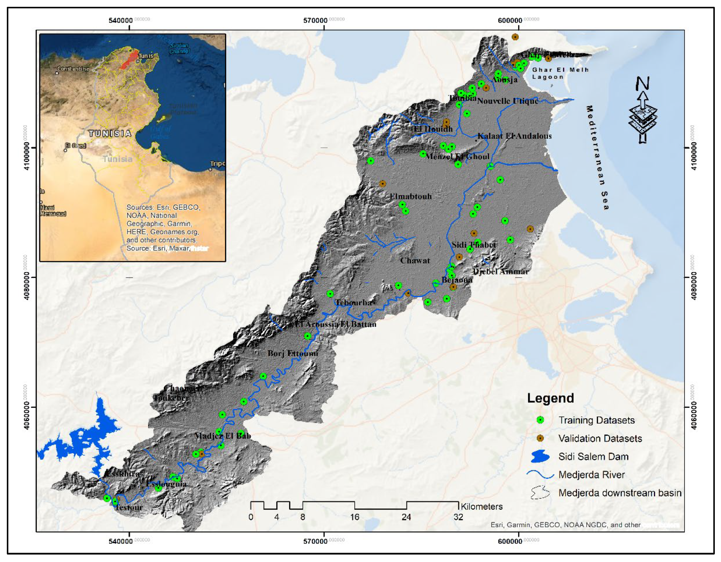
2.1. Study Area
2.2. Methodology and Datasets
2.2.1. Input Data
- Physico-chemical parameters
- Irrigation water quality Indices (IWQ)
2.2.2. Data Pre-Processing and Explanatory Data Analysis (EDA)
2.2.3. Machine Learning Modelling
- Artificial Neural Network (ANN)
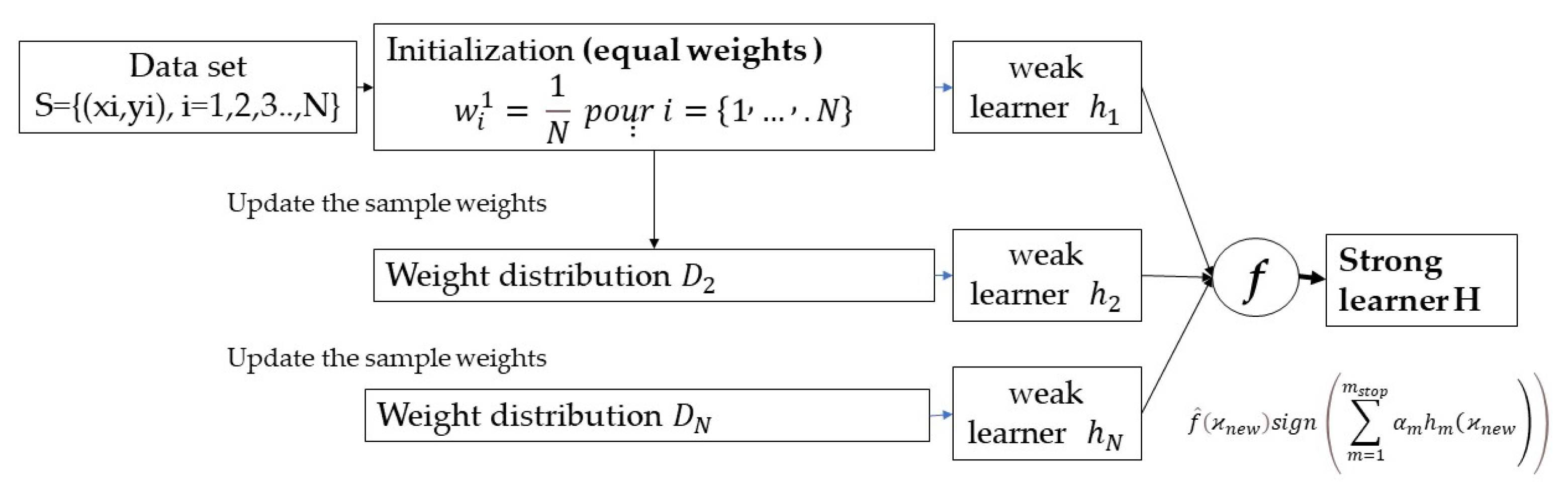
- Adaptive boosting model (AdaBoost)
- Support vector machine
- Random forest
2.2.4. Validation of Models Performance
- Metric validation
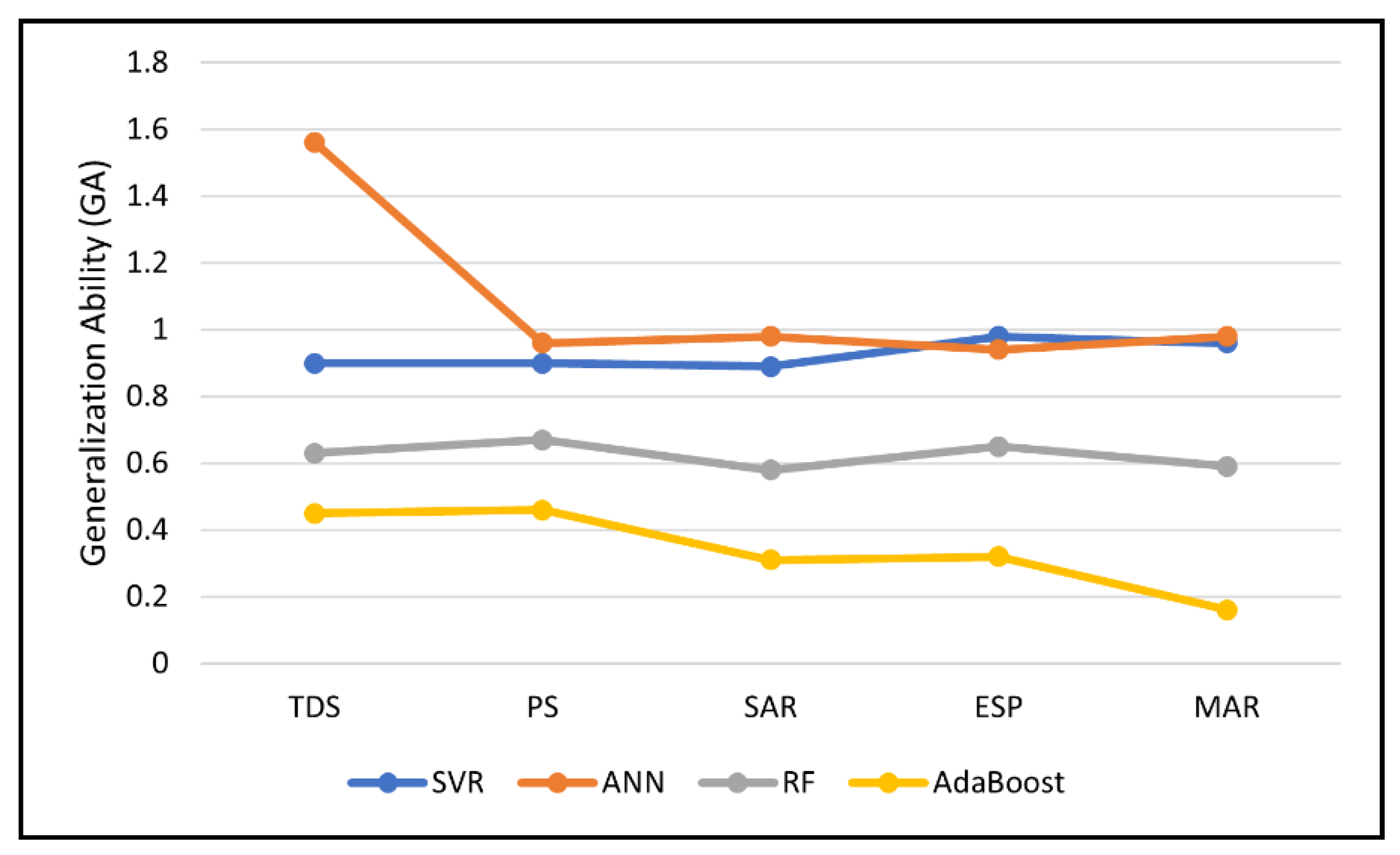
- Generalization ability
- Uncertainty and Sensitivity Analysis
3. Results
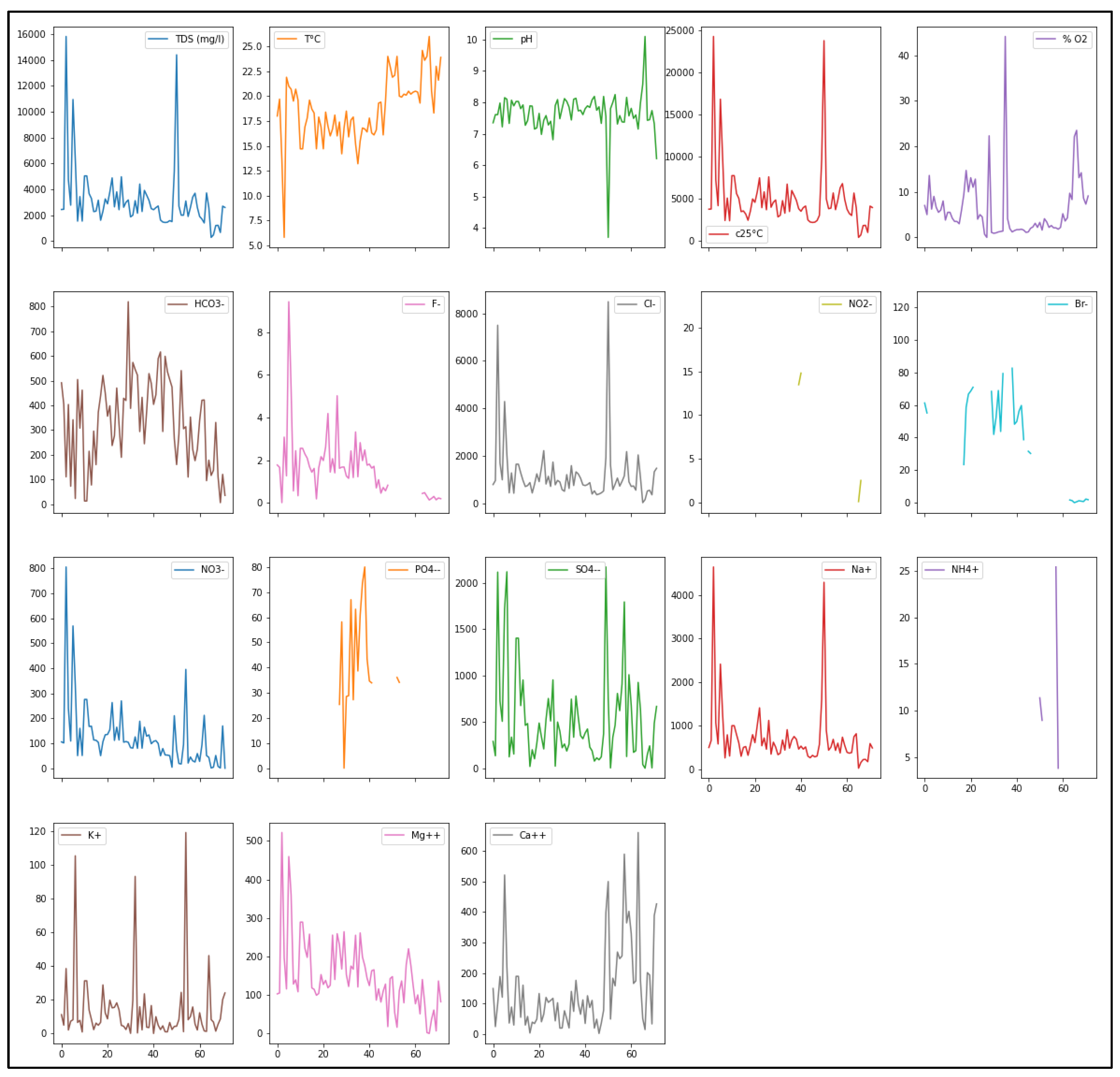
3.1. Statistical Analysis
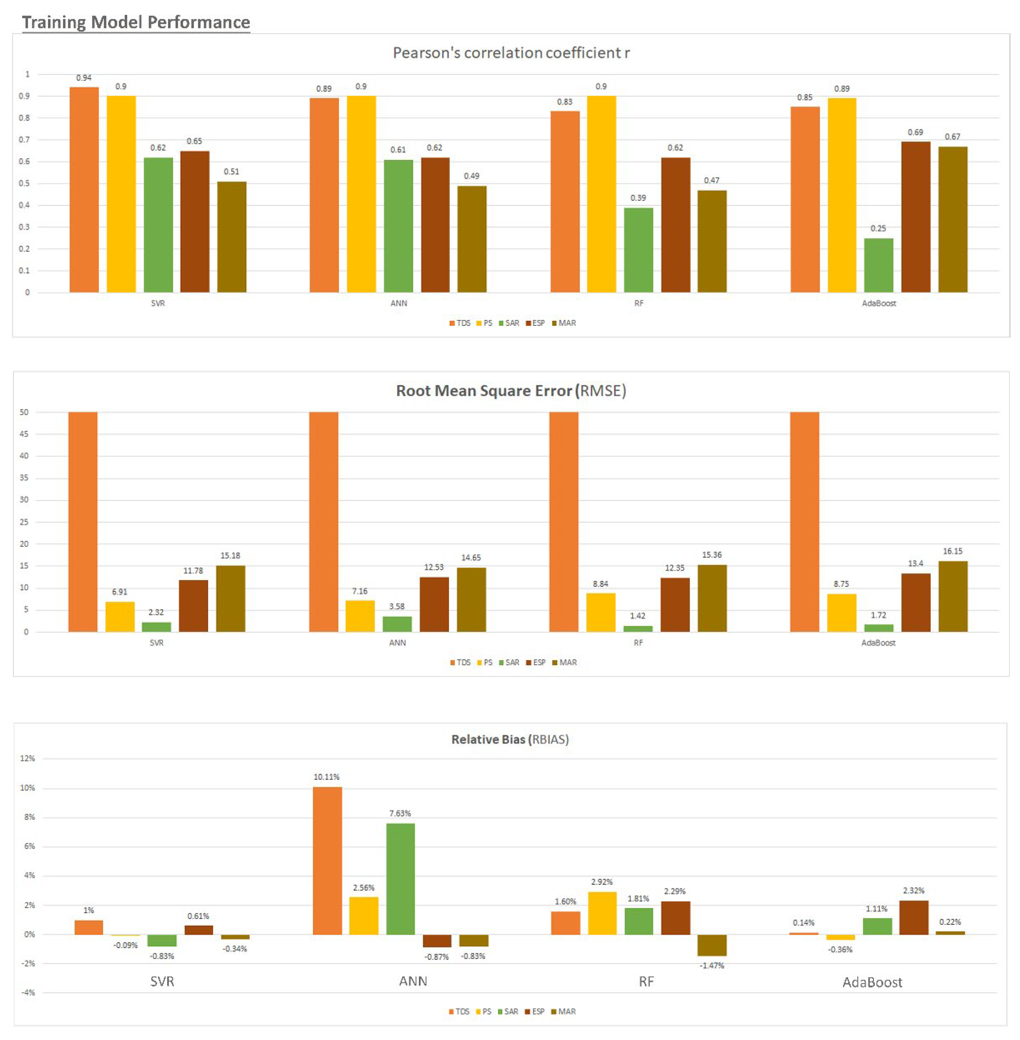
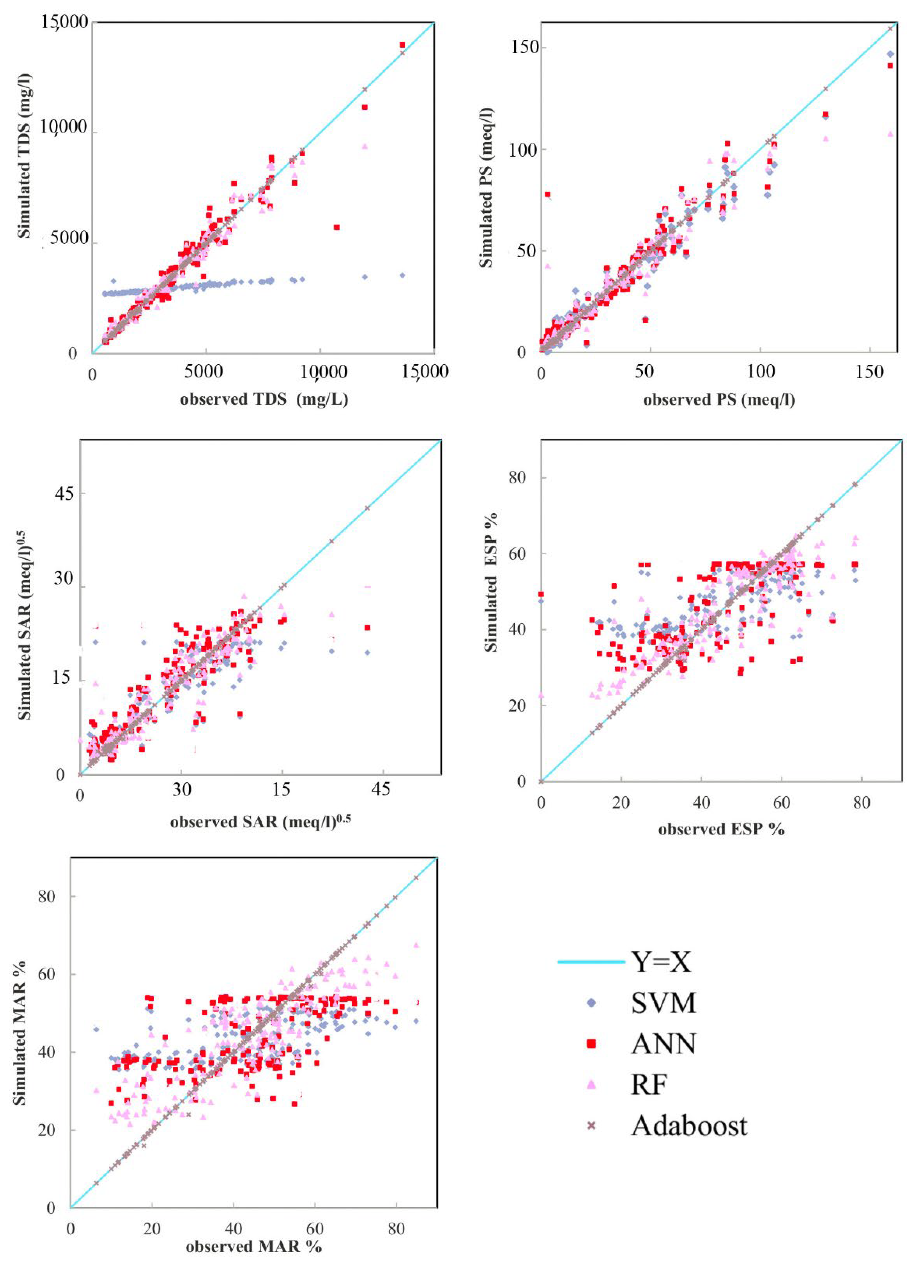
3.2. Implementation and Evaluation of Models
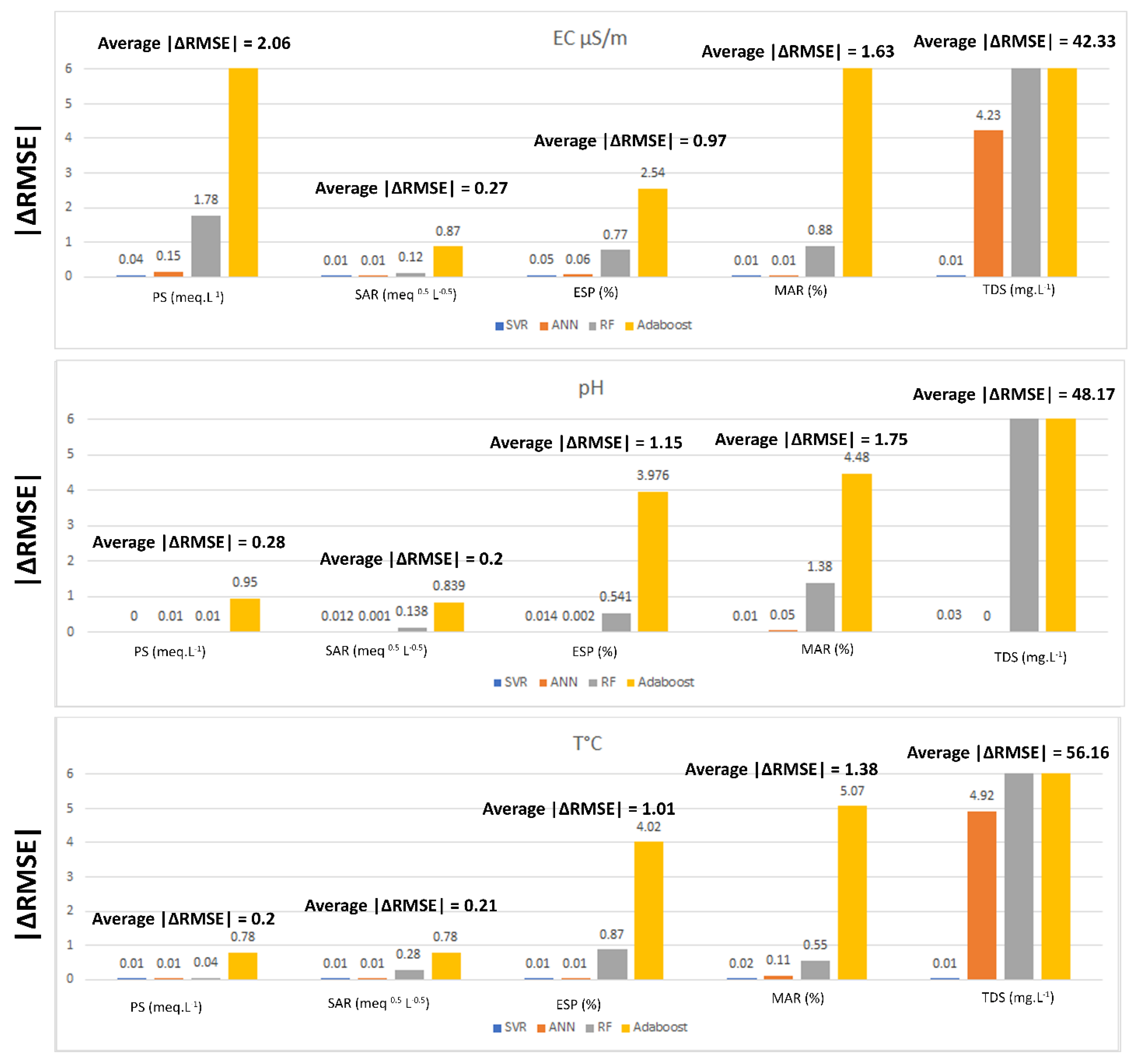
3.3. Uncertainty and Sensitivity Analysis
4. Discussion
5. Conclusions and Future Trends
Author Contributions
Funding
Institutional Review Board Statement
Informed Consent Statement
Data Availability Statement
Acknowledgments
Conflicts of Interest
References
- FAO. Water for Sustainable Food and Agriculture; Food and Agriculture Organization of the United Nations: Caracalla, Rome, 2017; ISBN 978-92-5-109977-3. [Google Scholar]
- Knaepen, H. Climate Risks in Tunisia Challenges to Adaptation in the Agri-Food System; European Centre for Development Policy Management (ECDPM): Maastricht, The Netherlands, 2021. [Google Scholar]
- Hssaisoune, M.; Bouchaou, L.; Sifeddine, A.; Bouimetarhan, I.; Chehbouni, A. Moroccan Groundwater Resources and Evolution with Global Climate Changes. Geosciences 2020, 10, 81. [Google Scholar] [CrossRef] [Green Version]
- Aureli, A.; Ganoulis, J.; Margat, J. Groundwater Resources in the Mediterranean Region: Importance, Uses and Sharing. Water Mediterr. 2008, 96–105. Available online: https://www.iemed.org/publication/groundwater-resources-in-the-mediterranean-region-importance-uses-and-sharing (accessed on 8 November 2021).
- Berhail, S. The impact of climate change on groundwater resources in northwestern Algeria. Arab. J. Geosci. 2019, 12, 770. [Google Scholar] [CrossRef]
- Rahmati, O.; Pourghasemi, H.R.; Melesse, A.M. Application of GIS-based data driven random forest and maximum entropy models for groundwater potential mapping: A case study at Mehran Region, Iran. CATENA 2016, 137, 360–372. [Google Scholar] [CrossRef]
- Yang, L.; Hua, G.; Caoab, L.; Wanga, X.; Chen, M.-H. A comparison of Monte Carlo methods for computing marginal likelihoods of item response theory models. J. Korean Stat. Soc. 2019, 48, 503–512. [Google Scholar] [CrossRef]
- Kopittke, P.M.; So, H.B.; Menzies, N.W. Effect of ionic strength and clay mineralogy on Na–Ca exchange and the SAR–ESP relationship. Eur. J. Soil Sci. 2006, 57, 626–633. [Google Scholar] [CrossRef]
- Wang, L.; Long, F.; Liao, W.; Liu, H. Prediction of anaerobic digestion performance and identification of critical operational parameters using machine learning algorithms. Bioresour. Technol. 2020, 298, 122495. [Google Scholar] [CrossRef]
- Paliwal, K.V. Irrigation with Saline Water; Water Technology Centre, Indian Agriculture Research Institute: New Delhi, India, 1972; p. 198. [Google Scholar]
- Amiri, V.; Rezaei, M.; Sohrabi, N. Groundwater quality assessment using entropy weighted water quality index (EWQI) in Lenjanat, Iran. Environ. Earth Sci. 2014, 72, 3479–3490. [Google Scholar] [CrossRef]
- Gorgij, A.D.; Kisi, O.; Moghaddam, A.A.; Taghipour, A. Groundwater quality ranking for drinking purposes, using the entropy method and the spatial autocorrelation index. Environ Earth Sci. 2017, 76, 269. [Google Scholar] [CrossRef]
- Bhagat, S.K.; Tiyasha, T.; Tung, T.M.; Mostafa, R.R.; Yaseen, Z.M. Manganese (Mn) removal prediction using extreme gradient model. Ecotoxicol. Environ. Saf. 2020, 204, 111059. [Google Scholar] [CrossRef]
- Leong, Y.C.; Hughes, B.L.; Wang, Y.; Zaki, J. Neurocomputational mechanisms underlying motivated seeing. Nat. Hum. Behav. 2019, 3, 1. [Google Scholar] [CrossRef]
- El Bilali, A.; Taleb, A.; Brouziyne, Y. Groundwater quality forecasting using machine learning algorithms for irrigation purposes. Agric. Water Manag. 2021, 245, 106625. [Google Scholar] [CrossRef]
- Evangelos, R. Machine learning, urban water resources management and operating policy. Resources 2019, 8, 173. [Google Scholar]
- Kim, H.; Kim, S.; Hwang, J.Y.; Seo, C. Efficient Privacy-Preserving Machine Learning for Blockchain Network. IEEE Access 2019, 7, 136481–136495. [Google Scholar] [CrossRef]
- Nolan, B.T.; Fienen, M.N.; Lorenz, D.L. A statistical learning framework for groundwater nitrate models of the Central Valley, California, USA. J. Hydrol. 2015, 531, 902–911. [Google Scholar] [CrossRef] [Green Version]
- Ransom, K.M.; Nolan, B.T.; Traum, J.A.; Faunt, C.C.; Bell, A.M.; Gronberg, J.A.M.; Wheeler, D.C.; Rosecrans, C.Z.; Jurgens, B.; Schwarz, G.E.; et al. A hybrid machine learning model to predict and visualize nitrate concentration throughout the Central Valley aquifer, California, USA. Sci. Total Environ. 2017, 601–602, 1160–1172. [Google Scholar] [CrossRef]
- Rodriguez-Galiano, J.A.V.F.; Luque-Espinar, M.; Chica-Olmo, M.P. Mendes, Feature selection approaches for predictive modelling of groundwater nitrate pollution: An evaluation of filters, embedded and wrapper methods. Sci. Total Environ. 2018, 624, 661–672. [Google Scholar] [CrossRef]
- Ouedraogo, I.; Defourny, P.; Vanclooster, M. Application of random forest regression and comparison of its performance to multiple linear regression in modeling groundwater nitrate concentration at the African continent scale. Hydrogeol. J. 2019, 27, 1081–1098. [Google Scholar] [CrossRef]
- Chen, H.K.; Chen, C.; Zhou, Y.; Huang, X.; Qi, R.; Shen, F.; Liu, M.; Zuo, X.; Zou, J.; Wang, Y.; et al. Ren Comparative analysis of surface water quality prediction performance and identification of key water parameters using different machine learning models based on big data. Water Res. 2020, 171, 115454. [Google Scholar] [CrossRef]
- Grbčić, L.; Lučin, I.; Kranjčević, L.; Družeta, S. Water supply network pollution source identification by random forest algorithm. J. Hydroinformatics 2020, 22, 1521–1535. [Google Scholar] [CrossRef]
- Bhagat, S.K.; Tung, T.M.; Yaseen, Z.M. Development of artificial intelligence for modeling wastewater heavy metal removal: State of the art, application assessment and possible future research. J. Clean. Prod. 2020, 250, 119473. [Google Scholar] [CrossRef]
- Lal, R.; Stewart, B.A. Soil Processes and Water Quality, 1st ed.; CRC Press: Boca Raton, FL, USA, 1994. [Google Scholar] [CrossRef]
- Zhu, S.; Hrnjica, B.; Ptak, M.; Choiński, A.; Sivakumar, B. Forecasting of water level in multiple temperate lakes using machine learning models. J. Hydrol. 2020, 585, 124819. [Google Scholar] [CrossRef]
- Ahmed, U.; Mumtaz, R.; Anwar, H.; Shah, A.A.; Irfan, R. Efficient water quality prediction using supervised machine learning. Water 2019, 11, 2210. [Google Scholar] [CrossRef] [Green Version]
- Fijani, E.; Barzegar, R.; Deo, R.; Tziritis, E.; Skordas, K. Design and implementation of a hybrid model based on two-layer decomposition method coupled with extreme learning machines to support real-time environmental monitoring of water quality parameters. Sci. Total Environ. 2019, 648, 839–853. [Google Scholar] [CrossRef]
- Lu, H.; Ma, X. Hybrid decision tree-based machine learning models for short-term water quality prediction. Chemosphere 2020, 249, 126169. [Google Scholar] [CrossRef]
- Bel Hadj Ali, S.; Trabelsi, F. CAJG-2020-P527: Saltwater Intrusion Vulnerability Mapping Using Multi-Model Ensemble of Machine Learning Algorithms: A Case Study of the Aousja Ghar El Melh Coastal Aquifer, Northeast of Tunisia; Advances in Science, Technology & Innovation (ASTI); Springer: Berlin/Heidelberg, Germany, 2022. [Google Scholar]
- Bel Hadj Ali, S.; Trabelsi, F. Impact of Anthropogenic Activities on the Groundwater Quality Using Machine Learning Algorithms: A Case Study of the Aousja Ghar El Melh Coastal Aquifer, Northeast of Tunisia. In Proceedings of the Mediterranean Geosciences Union Annual Meeting (MedGU-21), Istanbul, Turkey, 25–28 November 2021. [Google Scholar]
- Singh, R.; Kumar, S.; Nangare, D.D.; Meena, M.S. Drip irrigation and black polyethylene mulch influence on growth. Yield Water-Use Effic. Tomato 2009, 4, 1427–1430. [Google Scholar] [CrossRef]
- Wagh, V.M.; Panaskar, D.B.; Muley, A.A.; Mukate, S.V.; Lolage, Y.P.; Aamalawar, M.L. Prediction of groundwater suitability for irrigation using artificial neural network model: A case study of Nanded tehsil, Maharashtra, India. Model. Earth Syst. Environ. 2016, 2, 1–10. [Google Scholar] [CrossRef]
- Trabelsi, F.; LEE, S. GIS-based groundwater potential mapping using Machine learning models: Case of Medjerda aquifer, North of Tunisia. In Proceedings of the IAH2019, the 46th Annual Congress of the International Association of Hydrogeologists, Málaga, Spain, 22–27 September 2019. [Google Scholar]
- Trabelsi, F.; Ali, S.B.; Mukherjee, S.; Sipolya, R. Integrated Use of Satellite Remote Sensing and Hydraulic Modeling for the flood Risk Assessment at the middle valley of Medjerda. In Proceedings of the International Conference & Exhibition. Advanced Geospatial Science & Technology (TeanGeo 2016), Tunis, Tunisia, 26–28 September 2016. [Google Scholar]
- Ayed, B.N. Evolution Tectonique de l’Avant-Pays de la Chaîne Alpine de Tunisie du Début du Mésozoïque à l’Actuel Thèse d’Etat; Université de Paris Sud—Centre d’Orsay: Gif-sur-Yvette, France, 1986. [Google Scholar]
- Rouvier, H. Géologie de l’Extrême Nord-Tunisien: Tectonique et Paléogéographie Superposées à l’Extrémité Orientale de la Chaine Nord-Maghrébine. Thèse d’Etat, Paris, France, 1977; p. 307. [Google Scholar]
- Perthuisot, V. Dynamique et Pétrogenèse des Extrusions Triasiques en Tunisie Septentrionale. Thèse Doct, ès Science, Travelling Laboratory Geology Ecole North Superior, Paris, France, 1978; p. 312. [Google Scholar]
- Ghanmi, M. Etude géologique du J. Kebbouch (Tunisie septentrionale). Ph.D. Thesis, Thèse 3 ème Cycle, Toulouse, France, 1980; p. 141. [Google Scholar]
- Melki, F.; Zouaghi, T.; Chelbi, M.B.; Bédir, M.; Zargouni, F. "Role of the NE-SW Hercynian Master Fault Systems and Associated Lineaments on the Structuring and Evolution of the Mesozoic and Cenozoic Basins of the Alpine Margin, Northern Tunisia. In Tectonics—Recent Advances; IntechOpen: London, UK, 2012; Available online: https://www.intechopen.com/chapters/37864 (accessed on 8 November 2021).
- Trabelsi, F.; Mukherjee, S. Remote Sensing and GIS Techniques for Evaluation of Groundwater Quality in middle valley of Medjerda, Tunisia. In Proceedings of the 1st Euro-Mediterranean Conference for Environmental Integration (EMCEI), Sousse, Tunisia, 22–25 November 2017; p. 526. [Google Scholar]
- Trabelsi, F.; Mammou, A.B.; Tarhouni, J.; Piga, C.; Ranieri, G. Delineation of saltwater intrusion zones using the time domain electromagnetic method: The Nabeul–Hammamet coastal aquifer case study (NE Tunisia). Hydrol. Process. 2013, 27, 2004–2020. [Google Scholar] [CrossRef]
- Hachicha, M.; Cheverry, C.; Mhiri, A. The impact of long-term irrigation on change of groundwater level and soil salinity in northern Tunisia. Arid. Soil Res. Rehabil. 2010, 14, 175–182. [Google Scholar] [CrossRef]
- Chatti, A.; Trabelsi, F.; Arfaoui, A. Qualité et Vulnérabilité des Ressources en eau Souterraine de la Basse Vallée de la Medjerda; University of Jendouba: Jendouba, Tunisia, 2018. [Google Scholar]
- Breiman, L. Random Forests. Mach. Learn. USA 2001, 45, 5–32. [Google Scholar] [CrossRef] [Green Version]
- APHA. Standard Methods for the Examination of Water and Wastewater, 21st ed.; American Public Health Association/American Water Works Association/Water Environment Federation: Washington, DC, USA, 2005. [Google Scholar]
- Freund, Y.; Schapire, R.E. A Decision-Theoretic Generalization of On-Line Learning and an Application to Boosting. J. Comput. Syst. Sci. 1997, 55, 119–139. [Google Scholar] [CrossRef] [Green Version]
- Sorensen, D.L. Suspended and Dissolved Solids Effects on Freshwater Biota: A Review; US Environmental Protection Agency, Office of Research and Development: Washington, DC, USA, 1977.
- Richards, L.A. Diagnosis and Improvement of Saline Alkali Soils, Agriculture, 160, Handbook 60; US Department of Agriculture: Washington, DC, USA, 1954.
- Freeze, R.A.; Cherry, J.A. Groundwater; Prentice-Hall: Hoboken, NJ, USA, 1979. [Google Scholar]
- Raghunath, H.M. Groundwater; Wiley Eastern Ltd.: Delhi, India, 1987; p. 563. [Google Scholar]
- Barzegar, R.; Moghaddam, A.A.; Baghban, H. A supervised committee machine artificial intelligent for improving DRASTIC method to assess groundwater contamination risk: A case study from Tabriz plain aquifer, Iran. Stoch. Env. Res. Risk A. 2016, 30, 883–899. [Google Scholar] [CrossRef]
- Barzegar, R.; Adamowski, J.; Moghaddam, A.A. Application of wavelet-artificial intelligence hybrid models for water quality prediction: A case study in Aji-Chay River, Iran. Stoch. Env. Res. Risk A. 2016, 30, 1797–1819. [Google Scholar] [CrossRef]
- Barzegar, R.; Moghaddam, A.A. Combining the advantages of neural networks using the concept of committee machine in the groundwater salinity prediction. Model. Earth Syst. Environ. 2016, 2, 26. [Google Scholar] [CrossRef] [Green Version]
- Belayneh, A.; Adamowski, J.; Khalil, B.; Quilty, J. Coupling machine learning methods with wavelet transforms and the bootstrap and boosting ensemble approaches for drought prediction. Atmos. Res. 2016, 172, 37–47. [Google Scholar] [CrossRef]
- Dawson, C.W.; Wilby, R. An Artificial Neural Network Approach to Rainfall-Runoff Modelling. Hydrol. Sci. J. 1998, 43, 47–66. [Google Scholar] [CrossRef]
- Robert, J.S. Artificial Neural Networks by (1997-06-01) Hardcover–January 1; Mcgraw-hill Companies: New York, NY, USA, 1997. [Google Scholar]
- Castrillo, M.; García, A.L. Estimation of high frequency nutrient concentrations from water quality surrogates using machine learning methods. Water Res. 2020, 172, 115490. [Google Scholar] [CrossRef] [Green Version]
- Chen, K.; Chen, H.; Zhou, C.; Huang, Y.; Qi, X.; Shen, R.; Liu, F.; Cortes, C.; Vapnik, V. Support-Vector Networks. Mach. Learn. 1995, 20, 273–297. [Google Scholar] [CrossRef]
- Gayen, A.; Pourghasemi, H.R.; Saha, S.; Keesstra, S.; Bai, S. Gully erosion susceptibility assessment and management of hazard-prone areas in India using different machine learning algorithms. Sci. Total Environ. 2019, 668, 124–138. [Google Scholar] [CrossRef]
- Arlot, S.; Celisse, A. A survey of cross-validation procedures for model selection. Stat. Surv. 2010, 4, 40–79. [Google Scholar] [CrossRef]
- Rajaee, T.; Ebrahimi, H.; Nourani, V. A review of the artificial intelligence methods in groundwater level modeling. J. Hydrol. 2019, 572, 336–351. [Google Scholar] [CrossRef]
- Khalil, A.; Almasri, M.N.; McKee, M.; Kaluarachchi, J.J. Applicability of statistical learning algorithms in groundwater quality modelling. Water Resour. Res. 2005, 41, W05010. [Google Scholar] [CrossRef] [Green Version]
- Yoon, H.; Jun, S.C.; Hyun, Y.; Bae, G.O.; Lee, K.K. A comparative study of artificial neural networks and support vector machines for predicting groundwater levels in a coastal aquifer. J. Hydrol. 2011, 396, 128–138. [Google Scholar] [CrossRef]
- Qiu, Y.; Aufiero, M.; Wang, K.; Fratoni, M. Development of sensitivity analysis capabilities of generalized responses to nuclear data in Monte Carlo code RMC. Ann. Nucl. Energy 2016, 97, 142–152. [Google Scholar] [CrossRef] [Green Version]
- Patil, R.; Bellary, S. Machine learning approach in melanoma cancer stage detection. J. King Saud Univ.-Comput. Inf. Sci. 2020. [Google Scholar] [CrossRef]
- Islam, M.M.S.; Ferdous, Z.; Potenza, M.N. Panic and generalized anxiety during the COVID-19 pandemic among Bangladeshi people: An online pilot survey early in the outbreak. J. Affect. Disord. 2020, 276, 30–37. [Google Scholar] [CrossRef] [PubMed]
- Zhao, X.; Ning, B.; Liu, L.; Song, G. A prediction model of short-term ionospheric foF2 based on AdaBoost. Adv. Space Res. 2014, 53, 387–394. [Google Scholar] [CrossRef]
- Kardos, J.S.; Obropta, C.C. Water quality model uncertainty analysis of a pointpoint source phosphorus trading program. J. Am. Water Resour. Assoc. 2011, 47, 1317–1337. [Google Scholar] [CrossRef]
- Moreno-Rodenas, A.M.; Tscheikner-Gratl, F.; Langeveld, J.G.; Clemens, F.H.L.R. Uncertainty analysis in a large-scale water quality integrated catchment modelling study. Water Res. 2019, 158, 46–60. [Google Scholar] [CrossRef]
- Radwan, M.; Willems, P.; Berlamont, J. Sensitivity and uncertainty analysis for river quality modelling. J. Hydroinform. 2004, 6, 83–99. [Google Scholar] [CrossRef] [Green Version]
- Saghafi, H.; Arabloo, M. Modeling of CO2 solubility in MEA, DEA, TEA, and MDEA aqueous solutions using adaboost-decision tree and artificial neural network. Int. J. Greenh. Gas Control 2017, 58, 256–265. [Google Scholar] [CrossRef]
- Zhou, Z.; Feng, J. Deep Forest. Natl. Sci. Rev. 2019, 6, 74–86. [Google Scholar] [CrossRef] [PubMed]
- Di, M.Z.; Chang, P. Guo Water quality evaluation of the Yangtze River in China using machine learning techniques and data monitoring on different time scales. Water 2019, 11, 339. [Google Scholar] [CrossRef] [Green Version]
- Shojaei, M.; Nazif, S.; Kerachian, R. Joint uncertainty analysis in river water quality simulation: A case study of the Karoon River in Iran. Environ. Earth Sci. 2015, 73, 3819–3831. [Google Scholar] [CrossRef]
- Ayadi, A.; Ghorbel, O.; BenSalah, M.S.; Abid, M. A framework of monitoring water pipeline techniques based on sensors technologies. J. King Saud Univ.-Comput. Inf. Sci. 2022. [Google Scholar] [CrossRef]
- Chowdury, M.S.U.; Emran, T.; Ghosh, S.B.; Pathak, A.; Alam, M.M.; Absar, N.; Andersson, K.; Hossain, M.S. IoT based real-time river water quality monitoring system. Procedia Comput. Sci. 2019, 155, 161–168. [Google Scholar] [CrossRef]


| Parameter | Unit | Min | Max | Mean | Standard Deviation | Skew | Kurtosis |
|---|---|---|---|---|---|---|---|
| TDS | mg/L | 282.20 | 15,818 | 3167.72 | 2525.07 | 3.39 | 13.61 |
| T°C | °C | 5.80 | 26 | 18.65 | 0.67 | 3.40 | 13.06 |
| pH | 3.70 | 10.1 | 7.66 | 3996.26 | 3.08 | −0.41 | |
| EC | μs/cm | 348 | 24,300 | 4974.97 | 3996.26 | 3.40 | 13.69 |
| % O2 | 0.70 | 44.10 | 6.10 | 6.83 | 3.08 | 13.06 | |
| HCO3− | mg/L | 6.32 | 820.01 | 329.67 | 174.31 | 0.00 | −0.41 |
| F− | mg/L | 0.12 | 9.44 | 1.62 | 1.55 | 2.84 | 11.98 |
| Cl− | mg/L | 30.70 | 8492.67 | 1211.08 | 1306.23 | 4.18 | 19.80 |
| NO2− | mg/L | 0.03 | 22.94 | 7.81 | 7.88 | 0.64 | −1.18 |
| Br− | mg/L | 0.08 | 123.33 | 45.37 | 31.35 | −0.03 | −0.53 |
| NO3− | mg/L | 0.38 | 805.43 | 124.90 | 125.99 | 3.01 | 12.56 |
| PO42- | mg/L | 0.38 | 80.04 | 39.78 | 20.22 | 0.31 | −0.42 |
| SO42- | mg/L | 1.85 | 2173.01 | 530.36 | 505.27 | 1.76 | 2.99 |
| Na+ | mg/L | 19.52 | 4649 | 708.52 | 730.89 | 4.06 | 18.65 |
| NH4+ | mg/L | 3.79 | 25.44 | 12.39 | 8.02 | 1.30 | 2.21 |
| K+ | mg/L | 0.03 | 119.28 | 13.95 | 21.46 | 3.52 | 13.39 |
| Mg2+ | mg/L | 0.54 | 521.53 | 150.72 | 92.03 | 1.50 | 3.98 |
| Ca2+ | mg/L | 2.76 | 659.46 | 149.59 | 144.15 | 1.68 | 2.54 |
| Index Formula | Description |
|---|---|
[48] | The TDS is the sum of the ion concentrations in the water. |
[49] | SAR (sodium adsorption ratio) is a measure that determines the degree of hazard to crops by measuring the alkali/sodium risk. |
[50] | The potential salinity or Doneen is used for risk assessment of cations (calcium, sodium, and magnesium) and bicarbonates present in water that can affect soil permeability if used for long-term irrigation. |
[9] | The percent exchangeable sodium parameter (ESP in %) is used to evaluate the effect of sodium on soil texture. |
[51] | Residual sodium carbonates RSC indicate excess bicarbonate and carbonate in the irrigation water |
[52] | The excess of the concentration of magnesium, compared with the sum of the concentration of calcium and magnesium in water, affects the quality of soils that can translate into low crop yield. |
| Te | EC | TDS | pH | SAR | PS | ESP | MAR | |
|---|---|---|---|---|---|---|---|---|
| Mean | 18.65 | 4.97 | 31.68 | 7.66 | 9.60 | 39.68 | 57.32 | 63.17 |
| Standard error | 0.38 | 0.47 | 3.00 | 0.08 | 0.81 | 4.73 | 1.51 | 2.84 |
| Median | 18.45 | 3.91 | 26.00 | 7.75 | 7.76 | 28.52 | 56.16 | 71.26 |
| Mode | 14.70 | 3.71 | 50.38 | 7.61 | 10.65 | 13.78 | 56.05 | 85.25 |
| Standard deviation | d | 4.02 | 25.43 | 0.67 | 6.91 | 40.12 | 12.77 | 24.08 |
| Variance | 10.66 | 16.20 | 646.58 | 0.45 | 47.75 | 1609.57 | 163.18 | 579.90 |
| Kurstosis (kurtosis coefficient) | 2.28 | 13.69 | 13.61 | 18.36 | 13.01 | 16.94 | 0.62 | −0.64 |
| Skewness coefficient | −0.53 | 3.40 | 3.39 | −2.37 | 3.23 | 3.82 | 0.08 | −0.62 |
| Range | 20.20 | 23.95 | 155.36 | 6.40 | 42.66 | 246.14 | 64.90 | 93.03 |
| Minimum | 5.80 | 0.35 | 2.82 | 3.70 | 0.72 | 1.31 | 22.05 | 5.48 |
| Maximum | 26.00 | 24.30 | 158.18 | 10.10 | 43.38 | 247.44 | 86.95 | 98.51 |
| Model | Description of Parameters and Functions |
|---|---|
| ANN | 3 layers 12 neurons in hidden layer algorithm: Levenberg–Marquardt Function activation: sigmoid identity in output layer Epoch number: 1000 Learning rate: 0.01 Momentum coefficient: 0.85 |
| SVR | C = 200 Kernel function: RBF (γ = 1.2) ε-function loss, ε = 0.002 Gamma = 0.1 |
| Random Forest | Number of trees: 20 Loss function: exponential |
| AdaBoost | Estimator number: 50 Learning rate: 0.5 |
| Designation | Formula | Description |
|---|---|---|
| Pearson’s correlation coefficient (r) |
| |
| The root mean square error (RMSE) | A lower value of RMSE compared with the values of the results indicates a better fit of the model | |
| The relative bias (RBIAS). |
|
| Parameter | Error | ANN | SVR | RF | AdaBoost |
|---|---|---|---|---|---|
| TDS (mg L−1) | E | −27.01 | 412.48 | 4.79 | 11.57 |
| CB (95%) | 55.07 | 142.56 | 50.65 | 27.55 | |
| PS (meq L−1) | E | −0.27 | 0.45 | 0.21 | −0.09 |
| CB (95%) | 1.00 | 1.96 | 0.97 | 0.91 | |
| SAR (meq0.5 L−0.5) | E | −0.36 | 0.04 | −0.01 | −0.02 |
| CB (95%) | 0.47 | 0.57 | 0.09 | 0.04 | |
| ESP (%) | E | −1.31 | −1.45 | 0.13 | 0.56 |
| CB (95%) | 1.69 | 1.89 | 1.14 | 0.74 | |
| MAR (%) | E | −0.05 | 0.27 | −0.02 | 0.19 |
| CB (96%) | 2.01 | 2.47 | 1.47 | 0.69 |
Publisher’s Note: MDPI stays neutral with regard to jurisdictional claims in published maps and institutional affiliations. |
© 2022 by the authors. Licensee MDPI, Basel, Switzerland. This article is an open access article distributed under the terms and conditions of the Creative Commons Attribution (CC BY) license (https://creativecommons.org/licenses/by/4.0/).
Share and Cite
Trabelsi, F.; Bel Hadj Ali, S. Exploring Machine Learning Models in Predicting Irrigation Groundwater Quality Indices for Effective Decision Making in Medjerda River Basin, Tunisia. Sustainability 2022, 14, 2341. https://doi.org/10.3390/su14042341
Trabelsi F, Bel Hadj Ali S. Exploring Machine Learning Models in Predicting Irrigation Groundwater Quality Indices for Effective Decision Making in Medjerda River Basin, Tunisia. Sustainability. 2022; 14(4):2341. https://doi.org/10.3390/su14042341
Chicago/Turabian StyleTrabelsi, Fatma, and Salsebil Bel Hadj Ali. 2022. "Exploring Machine Learning Models in Predicting Irrigation Groundwater Quality Indices for Effective Decision Making in Medjerda River Basin, Tunisia" Sustainability 14, no. 4: 2341. https://doi.org/10.3390/su14042341
APA StyleTrabelsi, F., & Bel Hadj Ali, S. (2022). Exploring Machine Learning Models in Predicting Irrigation Groundwater Quality Indices for Effective Decision Making in Medjerda River Basin, Tunisia. Sustainability, 14(4), 2341. https://doi.org/10.3390/su14042341