Design of Supply Chain Transportation Pooling Strategy for Reducing CO₂ Emissions Using a Simulation-Based Methodology: A Case Study

Abstract

One of the main concepts for improving the sustainability of supply chains is the collaboration between stakeholders by increasing the efficiency of their shared resources. In the literature, there are many research papers related to vertical collaboration in the logistics industry. However, horizontal collaboration has not received the same degree of attention. In fact, horizontal collaboration such as shared freight carrier and freight consolidation can also be considered vital for low-carbon supply chain solutions. In this paper, the problem of the design of supply chain transportation pooling strategies (SCTPS) is studied, which considers both vertical and horizontal collaboration. The purpose of this paper is to study the impact of these SCTPSs to reduce CO₂ emissions using discrete-event simulation (DES)-based methodology. Using a numerical case study of two manufacturing companies and three customers, five SCTPS are studied including the following: (1) non-pooling strategy; (2) multi-pick strategy; (3) multi-drop strategy; (4) central hub strategy; and (5) combined hub and multi-drop strategy. The main result of the study is that all SCTPSs significantly reduce the CO₂ emissions compared to the non-pooled supply chain. In fact, the reduction in CO₂ emissions can reach 13% compared to the non-pooled strategy. Moreover, the best SCTPS that gives the minimum of CO₂ is the hub strategy, followed by the multi-pick strategy and the multi-drop strategy.

1. Introduction

The race toward mass industrialization that our society is currently experiencing and the great trend toward unbridled consumption are the main causes of the great climate change that we are undergoing. This significant change generates more frequent natural disasters that cause disruptions in the supply chain. Greenhouse gas (GHG) emissions caused by human activities are the main cause of this climate change, and as populations, economies, and living standards increase, the cumulative level of greenhouse gas emissions also increases. Moreover, recent researches show that also many consumers have low-carbon preferences [1].

The most abundant GHG is carbon dioxide CO₂, which is largely produced by the burning of fossil fuels, especially in logistics activities. In this context, the collaboration between supply chains has become essential. This collaboration improves the manager’s visibility and makes it easier to decide on the transport strategy to adopt in order to minimize the CO₂ emissions of his supply chain [2,3].

Supply chain transportation pooling strategy (SCTPS) is one of the innovative supply chain collaboration strategies. This concept goes much further than the simple idea of grouping vehicles, which is quite common in the professional world. It is essentially based on a partnership agreement that consists of voluntarily pooling and sharing resources (infrastructure, vehicles, etc.) and information from several supply chains with the aim of achieving a particular level of performance or gains [4]. Initially, the only opportunities perceived by supply chain managers in the concept of logistics resource pooling were purely economic. However, new and stricter ecology legislation has led them to consider the concept of combining logistics resources for environmental purposes, such as reducing CO₂ emissions [5,6].

1.1. Literature Overview

One of the main concepts for improving the sustainability of supply chains is the collaboration between stakeholders by increasing the efficiency of their shared resources [7,8,9,10]. There are two types of collaboration: vertical collaboration and horizontal collaboration. Vertical collaboration involves cooperation between stakeholders in the same supply chain, while horizontal collaboration includes cooperation between companies at the same level that can provide the same goods or services within a supply chain [11,12]. In the literature, there is a large amount of research related to vertical collaboration in the logistics industry [9,10,11]. However, horizontal collaboration such as shared freight carrier and freight consolidation has not received the same degree of attention [7,8,13], etc.

Over time, the concept of pooling logistics has been increasingly developed in the literature. Several research works are in line with collaboration approaches. Tuzkaya and nüt [14] addressed the problem of designing collaborative warehouses and transport networks through linear programming. The principal objective of their research was to determine the best strategy to distribute products from suppliers to a clustering hub and from this clustering hub to manufacturers. They looked at various constraints related to supplier and hub capacities, starting stock and backlog levels, transportation times, manufacturers’ demands, etc. The results of the linear programming model were compared for different scenarios. Further analyses were then performed by the authors to measure the sensitivity of the model results for different parameter values.

Ballot and Fontane [13] used an already optimized supply chain of a French distribution chain to study the possibility of further improving its performance using the logistic pooling strategy. The objective of the authors was to reduce the environmental impact of the supply chain by reducing transport emissions. The authors estimated CO₂ emissions from different empirical models of supply-pooling network strategies. The results showed a reduction in CO₂ emissions of about 25% with the new organizations. Qiu and Huang [15] study the pooling hub capacity across several supply chains using mathematical models and assess the impact of demand uncertainty on their financial performance measures. Two mathematical models were formulated for the studied supply chains. The first one does not consider the pooling hub, and the second one considers a pooling one. Therefore, the authors conducted different experiments to examine the clustering under different demand models and variances. The results show that the benefits of pooling hub capacity depend on the demand model. The results also indicate that demand variance can significantly influence the effect of central capacity pooling in terms of total supply chain costs. Leitner et al. [16] designed a centralized supply chain for automotive suppliers in Romania and Spain to reduce the cost of supply, CO₂ emissions, and increase transportation efficiency. The results of this study showed that the grouping of transport operations by the different partners generated a significant reduction in the number of trips, fuel consumption, and CO₂ emissions, in addition to transport costs.

Moutaoukil et al. [17] presented a pooling logistics model that takes into account the specificities of the agricultural and food supply chain flows. This model integrates the economic, environmental, and societal dimensions of the sustainable development objective. After identifying the different possible scenarios, the authors have shown the practical use of their proposal through the modeling of a particular scenario using a simulation technique to analyze the minimization of the total transport cost, the system’s CO₂ emissions, and the risk of accidents per million kilometers travelled by transporters. Pan et al. [18] explored the effect of combining supply chains on their CO₂ emissions with road and rail transport. They developed an optimization model with a piecewise linear objective function to assess quantitatively the impact of the products’ flows pooling on supply chains CO₂ emission. This model was then tested with real data for 12 weeks in a large distribution network composed of the supply chains of two French retailers. The overall results show a 14% reduction in CO₂ emissions with road transport and 52% with joint road and rail transport. Montoya-Torres et al. [19] conducted a case study through real data from the city of Bogotá, Colombia, for three companies in which each company has its own stores. They used mathematical modeling to compare the collaborative to the corresponding non-collaborative scenarios in terms of travel distance. In the non-collaborative scenario, each firm distributes goods to its own stores. While in the collaborative scenario the stores of the three companies are allocated to one of the three companies, serving as a pooling hub, and then routing is performed for each new allocation. On the basis of the obtained travel distances, the authors evaluated the travel time and carbon emission. The results highlight the quantitative benefits that can be obtained when pooling logistics operations are implemented, represented in both transportation costs and environmental impacts.

Ouhader and El kyal [7] tried to quantify the potential environmental and economic benefits of horizontal collaboration in transportation. Therefore, they studied the sensitivity between CO₂ emissions and transportation costs through an approach based on bi-objective mathematical modeling to minimize both the total transportation cost and the total environmental effect by simultaneously combining the location and routing decisions of the facility in urban freight distribution. The results of a noncollaboration scenario with the corresponding collaboration one showed that collaboration leads to a reduction in CO₂ emissions, transport costs, and distances traveled, in addition to the improvement of the vehicle load rate.

Habibi et al. [20] studied the problem of pooled hub location in the context of collaborative distribution network design in supply chains. The authors used two distribution networks of different supply chains to determine the best locations of the hubs that optimally serve their customers. Based on three collaborative cases and four cost-sharing strategies, the authors were able to verify whether collaboration offers a better decision and how to share the total cost between each supply chain to achieve a cost-effective solution.

Mrabti et al. [21] proposed a generic model of a pooled supply chain using discrete events simulation to assess economic indicators such as logistics cost, vehicles filling rate, and the environmental indicators CO₂ emissions. The authors then addressed a case study to examine the performance of the pooled supply chain strategy. This strategy was shown to reduce logistics cost, improve vehicle fill rate, and reduce CO₂ emissions.

Zouari [22] analyzed seven scenarios of logistic integration among a set of three companies in urban and interurban distribution. The main objective of this research was to choose the optimal path by showing the challenges and opportunities of pooling logistics. This resulted in reductions in transportation costs, congestion, and GHG emissions.

El Bouazzaoui et al. [23] discussed the concepts of transport and storage pooling in the Moroccan hydrocarbon supply chain. They studied the environmental impact of the pooling of resources used by the consolidation of transport trucks and storage tanks on the reduction of CO₂ emissions from different trucks from two companies. Based on real data of petroleum product flows over seven years from two major importers before and after resources pooling simulation models were developed to determine CO₂ emissions variation rates. The simulation results showed about 46% of the minimization of CO₂ emissions.

Gallardo et al. [24] applied an interdisciplinary transition innovation, management, and engineering methodology to the conceptualization, redesign, and redevelopment of the existing freight systems to achieve a downshift in CO₂ emissions.

In the literature, some research has studied CO₂ emission using simulation techniques in other areas. For instance, Sopha et al. [25] developed an integrated approach based on agent-based modeling and DES to evaluate CO₂ emission to decide between the existing evacuation plan for the Mount Merapi volcano eruption. Li and Lei [26] and Limsawasd and Athigakunagorn [27] applied DES in estimating and analyzing CO₂ emission construction engineering projects.

Moreover, in the literature, collaboration in supply chain have two types of benefits: economic benefits and environmental aspects benefits. A recent example of research is Gansterer et al. [9], which found that cost savings of 20–30% were made by carrier collaboration. The reduction in vehicle kilometers is demonstrated as a component of cost savings. However, Gansterer et al. [9] have not quantified explicitly the CO₂ emissions and the environmental aspect is not considered. In other examples [13,14,15,16,17,18,19,20,21,22,23,24,25,26,27,28], the GHG emissions is explicitly studied as benefits of supply chain collaboration.

1.2. Objectives and Contributions of the Study

Based on the literature review, this research starts from two major assertions. First, the majority of previous research in supply chain transportation pooling strategy (SCTPS), which can also be named freight consolidation, have studied the impact of only one type of SCTPS on the supply chain performances. Second, most of the previous research is related to vertical collaboration in the supply chain and rarely to horizontal collaboration. To fil this gap, the present research is about analyzing the effect of various SCTPS to reduce CO₂ emissions using discrete event simulation (DES). In fact, the studied problem of SCTPS design considers both vertical and horizontal collaboration.

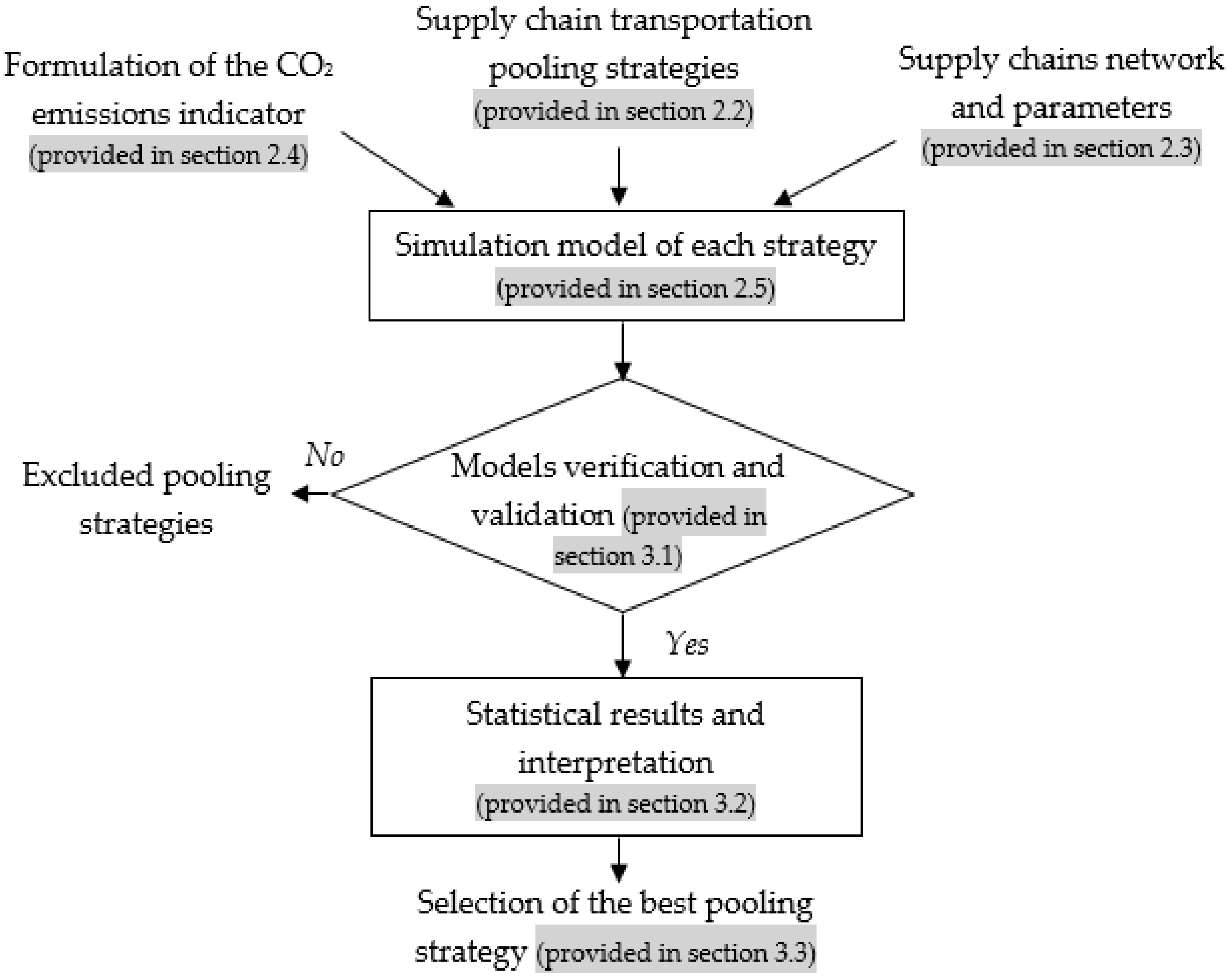
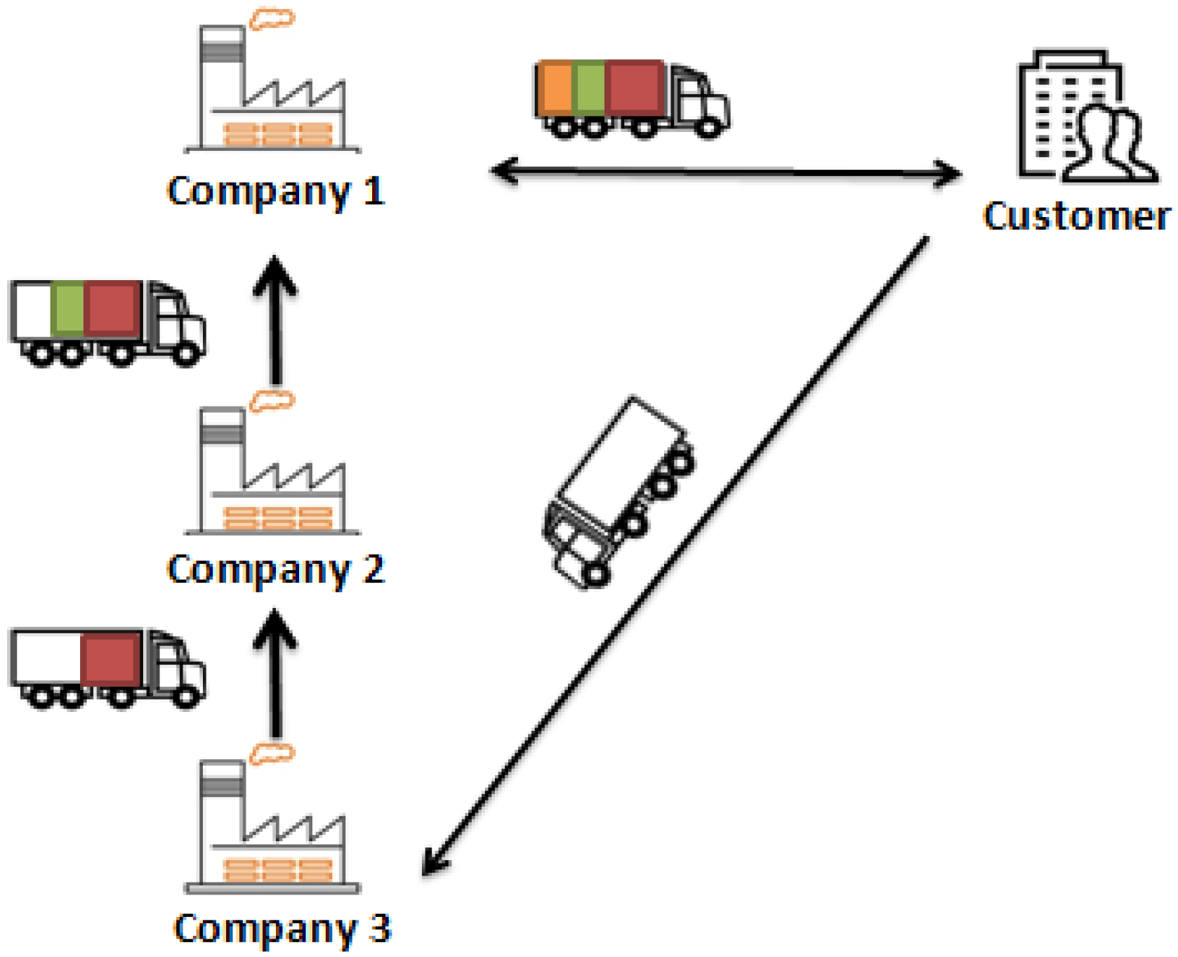
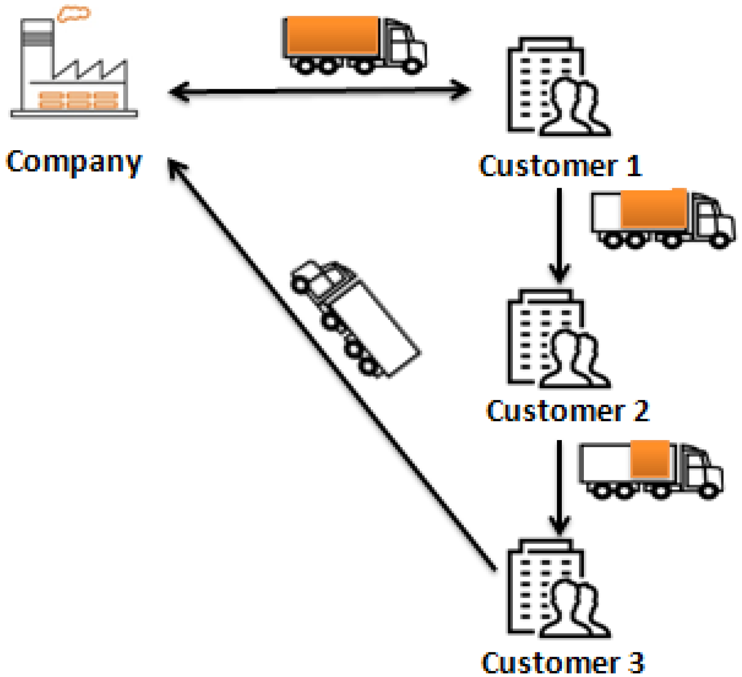
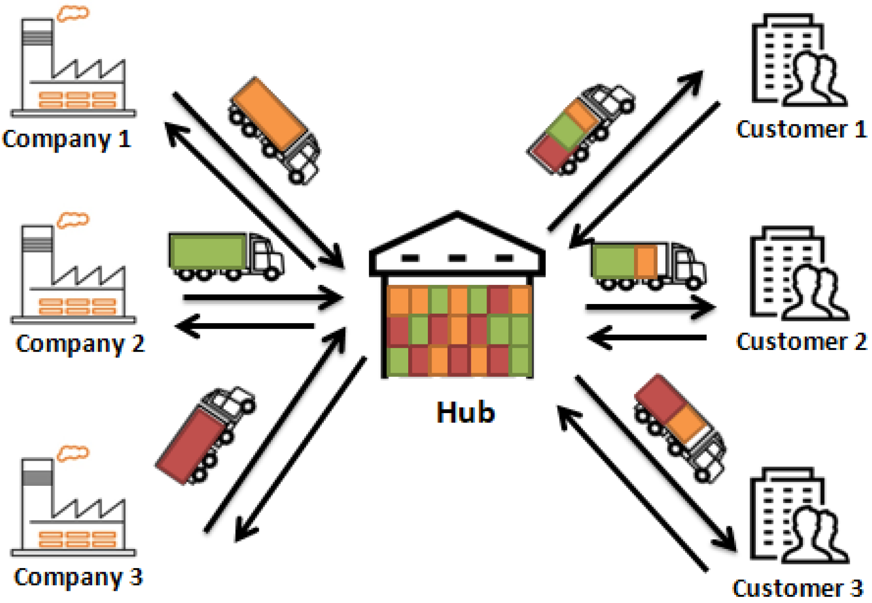
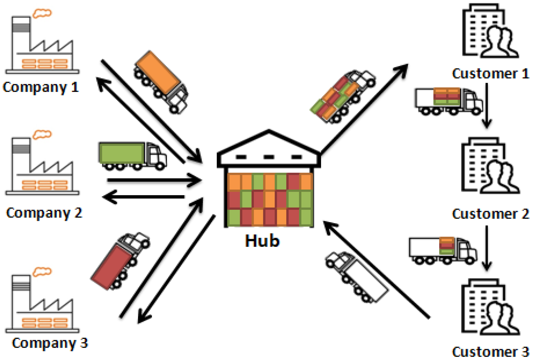
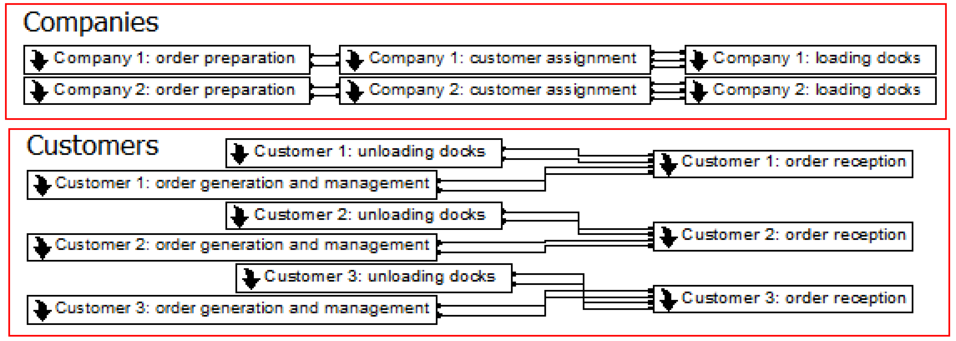
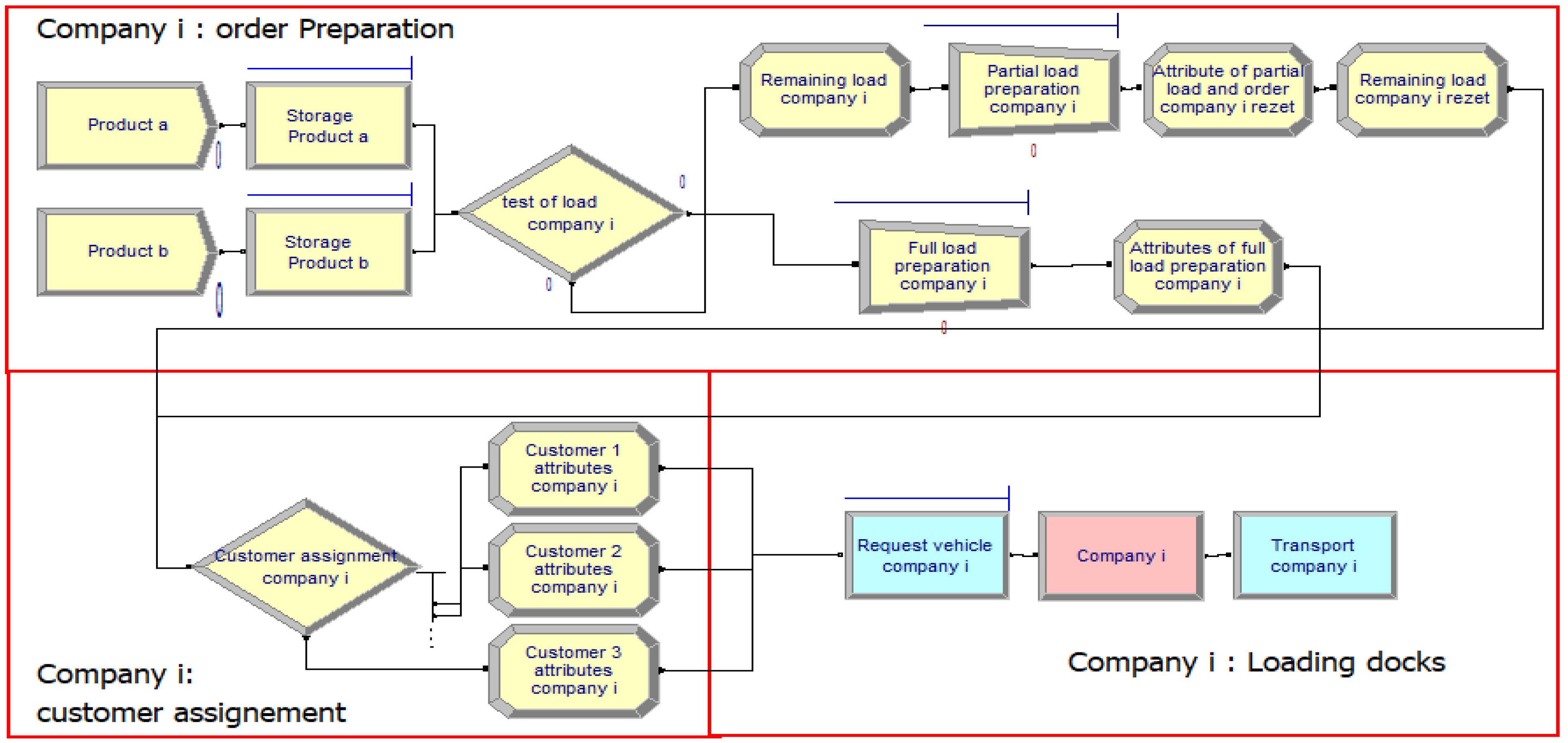
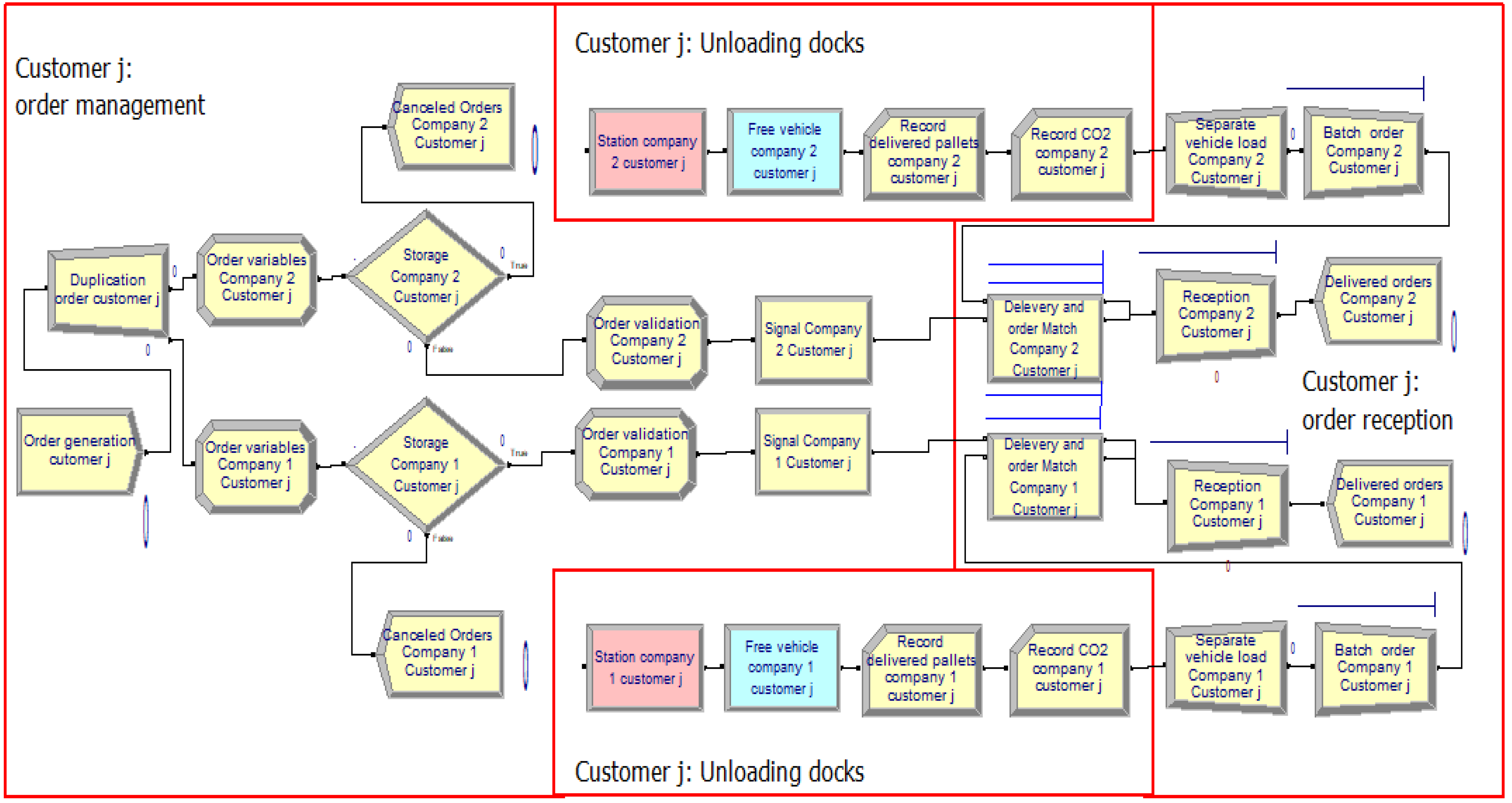
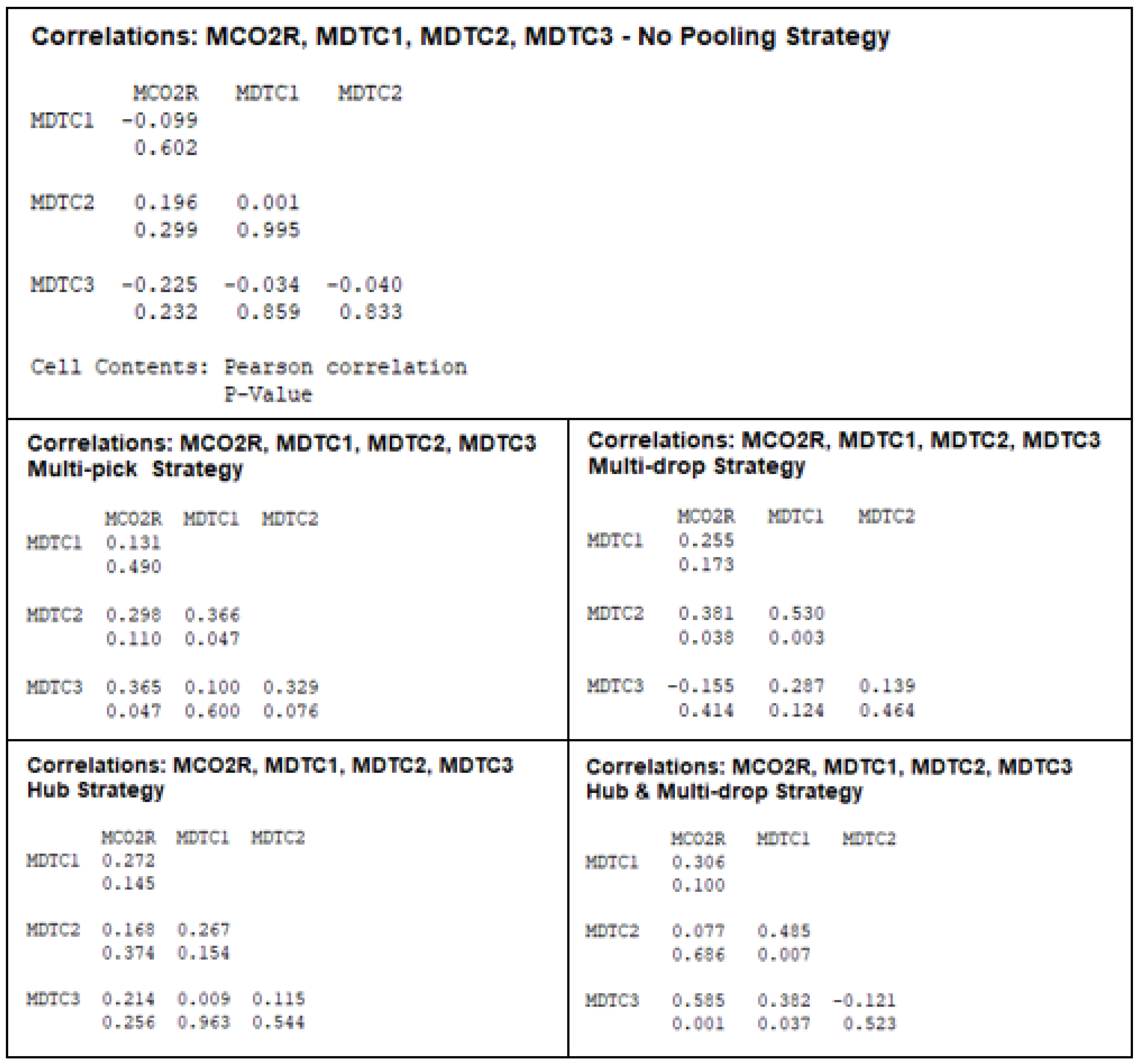
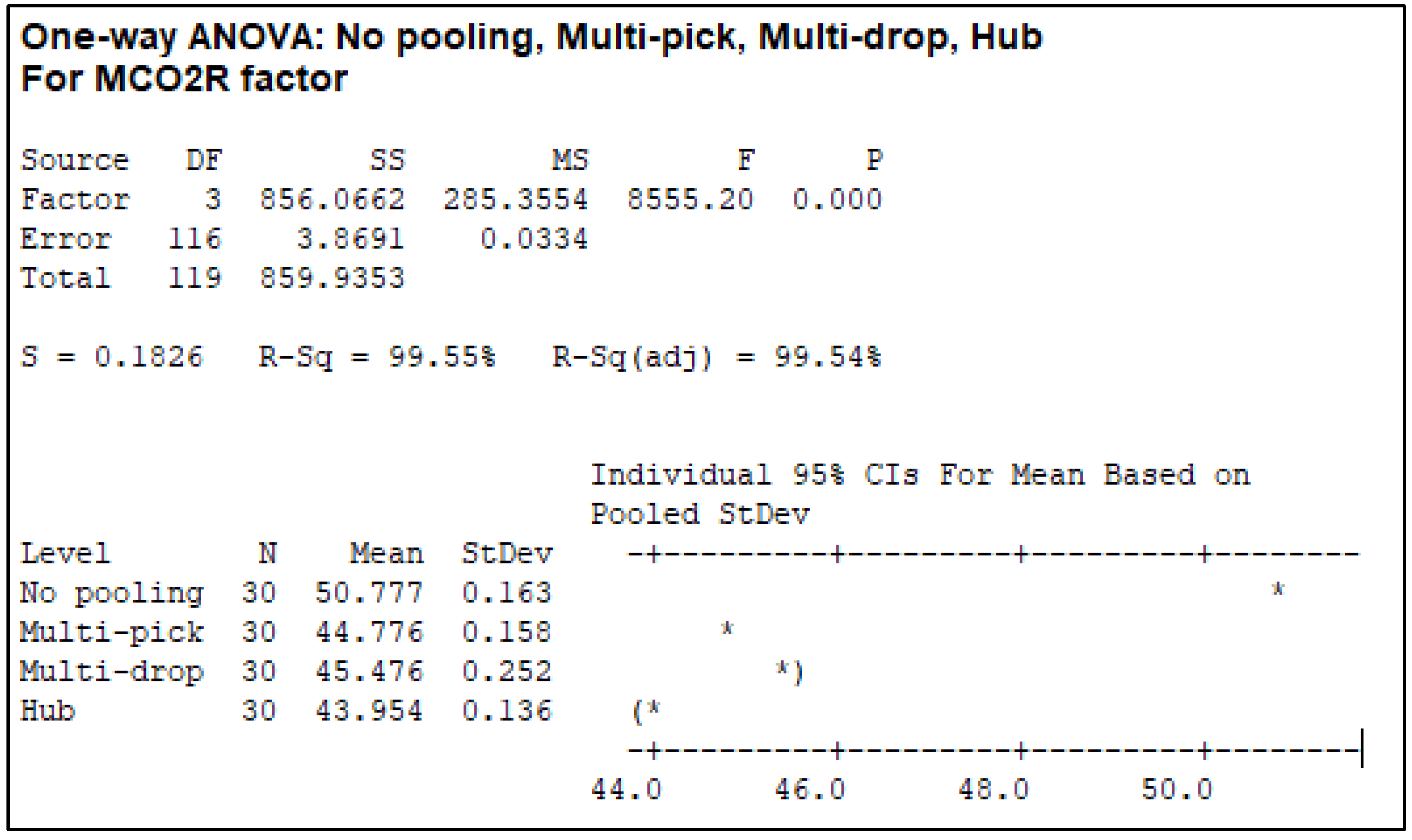
The studied supply chain is a network between two manufacturing companies and three customers and its suppliers to produce and distribute four product types. Five SCPS are studied and include the following: (1) non-pooling strategy; (2) multi-pick strategy; (3) multi-drop strategy; (4) central hub strategy; and (5) combined hub and multi-drop strategy. For each studied strategy, a three-step approach is applied. First, a simulation model for the strategy is developed using Siman/Arena software. Second, the verification and validation of the simulation model are based on the Pearson correlation test between CO₂ emissions and the mean delivery time of each customer and between the mean delivery time of each pair of customers. Third, one-way analysis of variance (ANOVA) and Games-Howell simultaneous confidence intervals are used to interpret simulation results. The main result of the study, which will be obtained in the end, is that all SCTPSs significantly reduce CO₂ emissions compared to the non-pooled supply chain.

2. Materials and Methods

2.1. The Applied Approach

The flowchart of the applied approach in this research is presented in Figure 1. To prepare the simulation model of each strategy, three inputs must be prepared. First, all supply chain transportation pooling strategies are described and provided in Section 2.2. Second, the studied supply chains network and parameters are presented in Section 2.3. Third, the formulation of the CO₂ emissions indicator is provided in Section 2.4. After the models’ verification and validation, which are provided in Section 3.1, some of the studied strategy can be excluded from the comparative analysis. This step of verification and validation of the simulation models are based on the Pearson correlation test between CO₂ emissions and the mean delivery time of each customer and between the mean delivery time of each pair of customers. The statistical analysis of the simulation results is provided in Section 3.2. One-way analysis of variance (ANOVA) and simultaneous Games-Howell confidence intervals are used to interpret simulation results. Finally, the selection of the best pooling strategy is provided in Section 3.3.

2.2. Supply Chains Transportation Pooling Strategies

Many definitions of transportation pooling exist. However, they all maintain that it is a partnership agreement between multiple actors that consists of the voluntary pooling of physical resources, information, and skills with the aim of obtaining economic, ecological, and financial collective benefits that they could not produce individually. The framework of this cooperation can take different organizational forms depending on the nature of the parties, the means, and the products or services.

2.2.1. Supply Chains with a Multi-Pick Pooling Strategy (Pick-Up Round)

This strategy involves consolidating supplies destined for the same delivery site (customer) from multiple shipping locations (suppliers). Therefore, orders intended for the same customer from multiple suppliers must be grouped through a pickup round performed by one or more vehicles [29]. Figure 2 presents a conceptual supply chain with multi-pick.

2.2.2. Supply Chains with Multi-Drop Pooling Strategy (Distribution Round)

Multi-drop strategy is based on the same logic as multi-pick, except that the consolidating starts from a single shipping location and goes to multiple delivery sites. One or more vehicles leave from the same supplier to transport different orders and deliver them successively to several customers through a distribution round. These customers are geographically close or are on the same transport line [29,30]. Figure 3 presents a conceptual supply chain with multi-drop.

2.2.3. Supply Chains with Pooling Hub Strategy

One or more shared intermediary hubs are integrated into the supply chain structure. Deliveries are then made in two stages, with suppliers routing their products to the shared hub, and when a customer sends them their delivery requirements, they send the order to the shared hub to make the delivery. Incorporating the hub into the supply chain structure increases the size of shipments and improves transportation costs by increasing vehicle fill rates [31]. Figure 4 presents a conceptual supply chain with central hub.

2.2.4. Supply Chains with Pooling Hub and Multi-Drop Delivery Strategy

This strategy is a combination of the two previous pooling strategies. Deliveries upstream of the hub follow the same form. However, deliveries downstream of the hub are made using the multi-drop technique. Therefore, these deliveries are made by distribution rounds between the pooling hub and the customers [30,31]. Figure 5 presents a conceptual supply chain with combined hub and multiple drops.

Five strategies are studied in this work, as presented in

Table 1. Description of the five supply chain pooling strategies.

Type	Strategy	Relation between Customers	Description
Non-pooling strategy		No
Pooling	Multi-pick	No	Figure 2
	Multi-drop	Yes	Figure 3
	Hub	No	Figure 4
	Hub and multi-drop	Yes	Figure 5

.

2.3. Supply Chain Network and Parameters

This study adopts a pooled supply chain composed of two companies and three customers. Companies feed the supply chain with products according to statistical distributions, which are summarized in

Table 2. Time and quantity of pallet feeding in supply chain.

		Inter-Arrival Time (Hour)	Palettes Quantity
Company 1	Product 1	N (4, 0.5)	2
	Product 2	N (3, 0.5)	2
Company 2	Product 3	N (3.5, 0.5)	2
	Product 4	N (3.5, 0.5)	2

N: Normal distribution.

. Every customer submits a delivery order to both companies at different times. These order times and the corresponding quantity of pallets for each type of product follows discrete distributions (

Table 3. Time between orders and quantity of pallets per order.

	Time Between Order	Quantity of Pallets Per Order
Customer 1	Unif (12, 24)	Company 1	Product 1	DISC (0.6, 4, 1.0, 5)
			Product 2	DISC (0.3, 5, 1.0, 7)
		Company 2	Product 3	DISC (0.8, 6, 1.0, 7)
			Product 4	DISC (0.7, 4, 1.0, 6)
Customer 2	Unif (12, 24)	Company 1	Product 1	DISC (0.4, 4, 1.0, 5)
			Product 2	DISC (0.6, 5, 1.0, 7)
		Company 2	Product 3	DISC (0.5, 3, 1.0, 5)
			Product 4	DISC (0.8, 4, 1.0, 6)
Customer 3	Unif (24, 36)	Company 1	Product 1	DISC (0.5, 3, 1.0, 6)
			Product 2	DISC (0.5, 4, 1.0, 8)
		Company 2	Product 3	DISC (0.3, 3, 1.0, 6)
			Product 4	DISC (0.3, 6, 1.0, 8)

DISC: discrete distribution, Unif: Uniform distribution.

). All the distances between the components of the supply chain are defined in kilometers in

Table 4. Distances and speeds in the pooled supply chain.

Hub	*
Company 1	D:35 v:40	*
Company 2	D:46 v:40	D:11 v:40	*
Customer 1	D:155 v:80	D:190 v:80	D:201 v:80	*
Customer 2	D:180 v:80	D:210 v:80	D:221 v:80	D:20 v:40	*
Customer 3	D:245 v:80	D:280 v:80	D:291 v:80	D:90 v:80	D:55 v:40	*
	Hub	Company 1	Company 2	Customer 1	Customer 2	Customer 3

D: distance in kilometers, v: speed in kilometers per hour, * not possible.

. The average speeds of the delivery vehicles are defined according to the location of the shipment and destination. In the case of long distances, the average speed of the vehicle has been set at 80 km per hour. For small and medium distances, speeds have been reduced to 40 km per hour (Table 4). The choice of vehicles’ load was based according to the French Environment and Energy Management Agency (ADEME) [32,33]. The chosen vehicle is a 12-tonne Gross Vehicle Weight Rating (GVWR) truck. The maximum loading capacity was limited to 6 tons due to pallet volume constraints. Each company has two trucks in its fleet. These trucks are then distributed between the companies and the pooling hub in the case of the pooled supply chains with hub models. Therefore, in these models, the companies operate one truck in common to deliver their pallets to the pooling hub. The other three trucks are assigned to the pooling hub for deliveries to customers.

2.4. Formulation of the CO₂ Emissions Indicator

Tundys and Winiewski [34] affirmed that the important element to reduce the negative environmental impact of chains is a well-thought-out relationship with suppliers, a well-chosen and adapted logistics infrastructure, including means of transport. In this research, only the CO₂ emissions related to the transport means is considered. Other sources of CO₂ emissions related to product manufacturing, storage, etc., are not considered because it is assumed to be the same for all studied pooling strategies.

Moreover, in the literature there are two main methods used to estimate supply chain emissions: the spend-based method and the activity-based method [35]. The spend-based method is not used because it takes the financial value of an equipment and multiplies it by an emission factor. Then, the method used in this research is the activity-based method.

For the formulation of the emissions indicator of CO₂, the works of Mrabti et al. [36,37] were used as a basis. These emissions depend on the weight of the transported load, the capacity of the vehicle, and the travelled distance. Hence, the formulas for estimating CO₂ emissions for a delivery are presented in Equations (1) and (2):

E_loaded = D_ij × [E_empty + (E_full − E_empty) × X],

(1)

E_unloded = D_ij × E_empty,

(2)

With

• E_loaded: The total CO₂ emission of a loaded vehicle, in KgCO₂, between nodes i and j.
• E_unloaded: The total CO₂ emission of an unloaded vehicle, in KgCO₂, between nodes i and j.
• D_ij: The distance, in kilometers, between nodes i and j.
• E_empty: The CO₂ emission rate, in KgCO₂/Km, of an empty vehicle.
• E_full: The CO₂ emission rate, in KgCO₂/Km, of a full loaded vehicle.
• X: The ratio between weight of the load of merchandise and the maximum payload of the vehicle.

The CO₂ emission rates of empty and fully loaded vehicles, E_empty and E_full, are related to the vehicle speed as follow [37]:

E_empty = K+ a × v + b × v² + c × v³ + d/v + e/v² + f/v³,

(3)

E_full = E_empty × C_load(v),

(4)

C_load(v) = k + r × v + s × v² + t × v³ + u/v,

(5)

With

• v: The vehicle speed
• K and k: Constants determined according to the Gross Vehicle Weight Rating (GVWR).
• a, b, c, d, e, f, r, s, t, u: Coefficients determined according to the vehicle GVWR.
• C_load: The load correction factor

Based on the GVWR of the truck and the Equations (3) and (4), the values of full and empty emission rates are estimated [37,38]. The values obtained are E_empty = 0.48 KgCO₂/km and E_full = 0.58 Kg CO₂/km for the 40 km/hour speed and E_empty = 0.51 KgCO₂/km and Efull = 0.58 KgCO₂/km for the 80 km/hour speed. An average load capacity of 9.79 tons was adopted for each truck [32]

2.5. Simulation Models

All simulation models are developed using the Arena 14.0 commercial simulation software. This tool integrates all the functions needed for simulation including animation, analysis of input, and output data. The simulation model of the non-pooled supply chain is fully detailed in the next subsection. However, the others simulation models of the pooled strategies can be founded in the supplementary file.

2.5.1. Non-Pooled Supply Chain Model

The structure of the non-pooled supply chain model is composed of two parts: companies and customers. The first part contains two sub-models, each corresponding to one company. The second part contains three sub-models each corresponding to a customer (Figure 6).

Every company sub-model is composed of the three sections “Company i: order preparation”, “Company i: customer assignment”, and “Company i: loading docks” (Figure 7). The first section “Company i: order preparation” acts as a generator of pallets of products and manages the order preparation. Every company produces two types of products for which as many “Create” modules are lined up. Each pallet of products is placed on hold in a storage area materialized by a “Hold” module waiting for an order from customers. In this case, the corresponding customer sends a signal to the appropriate “Hold” module to release the necessary number of pallets. These pallets pass through a “Decide” module to check whether their number matches the loading capacity of the transport vehicles. If this variable is greater than or equal to the vehicle loading capacity, pallets corresponding to this capacity are grouped into a full load by the module “Volume load preparation company” “Batch”. This load passes then through an “Assign” module where it receives different attributes and variables referring to the load size and the order size. The order size variable is then reduced by the number of pallets already grouped. In contrast, if the load matching condition is not verified, all the pallets are sent to the “Partial load preparation company i” “Batch” module. But before, a variable referring to the remaining part of the order is incremented by passing these pallets through the “Assign” module named “Remaining load company i”. Next, this load passes through other “Assign” modules to receive the new value of the load size attribute and reset all the other variables.

In the second section “Company i: Customer Assignment”, each delivery is assigned to the corresponding customer through a “Decision” module. This module is connected to three “Assign” modules, each corresponding to one customer. In these modules, necessary attributes, such as order number, the number of pallets, and the delivery sequence, are assigned to each delivery before it is loaded into a vehicle. The stations that make up each of the delivery sequences are previously defined in the “sequence” modules.

Each delivery is made to wait in the queue of a “Request” module for the nearest free vehicle in the third section named “Company i: Loading docks”. This vehicle collects the shipment from the station “Company I” and passes to the “Transport” module, where the speed of the trip is defined, to be finally sent to its corresponding customer.

As for the company sub-model, each customer “j” sub-model comprises three sections named “Customer j: order generation and management”, “Customer j: unloading dock”, and “Customer j: order reception” (Figure 8).

In the “Customer j: order generation and management” section a “Create” module generates delivery orders. These orders are duplicated according to the number of companies through a “Separate” module called “Duplication order customer j”. Each copy of this order is then transferred to an “Assign” module. Each of these modules will increment the number of orders and assign the value of ordered pallet number per type of product to the order. Then, every order goes through a “Decide” module, named “Storage Company i Customer j” to verify the availability of the pallet in the storage of the companies. If availability is verified, the order is validated and goes through a “Signal” module to send a signal to the corresponding company to release the requested number of pallets. If the storage availability is not verified, the order will be cancelled for unavailable storage and will be filed in a “Dispose” module.

Each vehicle, entering the section “Customer j: loading docks”, is sent to the “Free” module. This module frees the vehicles from their loads, which are forwarded to “Record” modules. The first one is used to store the total number of delivered pallets, while the second one is used to calculate CO₂ emissions rate.

In the section “Customer j: order reception”, each delivered load is split into individual pallets by a “Separate” module. These pallets are sent to a “Batch” module, whose function is to group all the pallets of each order. Once all the ordered pallets are regrouped, a “Match” module matches them with the corresponding order. To validate the reception of the order, the matched informational (order) and physical (pallets) flows are grouped together by a “Batch” module and removed from the system via a “Dispose” module.

2.5.2. Pooled Supply Chains with Multi-Pick Model

This simulation model has the same structure as the non-pooled simulation model, except for the companies’ sub-models. Indeed, a new section, which manages the flow of multi-pick deliveries, appears in these sub-models. Moreover, each company sub-model has a different structure from the other. For more details about this simulation model, the reader can consult Figure S1 in the Supplementary Material.

2.5.3. Pooled Supply Chains with Multi-Drop Model

In this simulation model, each company must manage the joint delivery of several parts to different customers. For this purpose, a new section named “Company i: multi-drop management” appears in each company sub-model. In addition, the customers must manage the reception of their corresponding partial loads of these multi-drop deliveries and the dispatch of the other partial loads to their customers. This is the role of the section “Customer j: multi-drop management”. These sections differ from customer 1 to other customers since it is the closest to the companies and must manage the reception and the dispatch of more partial loads. For more details about this simulation model, the reader can consult Figure S2 in the Supplementary Material.

2.5.4. Pooled Supply Chains with Hub Model

In contrast to the previous models, this model consists of three sub-models: the production companies’ sub-model, which contains two sections each corresponding to one company, the customers’ sub-model, which contains three sections each corresponding to one customer, and the pooling hub sub-model. Intermediary deliveries are directed from the companies to the pooling hub, which in turn is responsible for supplying all the customers. For more details about this simulation model, the reader can consult Figure S3 in the Supplementary Material.

2.5.5. Pooled Supply Chains with Hub and Multi-Drop Model

Different modifications are necessary with the hybridization between the multi-drop delivery policy and the pooling hub. These modifications are mainly concentrated on the sub-models of the pooling hub. Indeed, this section integrates a new “Hub: multi drop management” sub-section, which is based on the operating mode of the “Company j: multi drop management” one in the pooled supply chain with multi-drop simulation model. For more details about this simulation model, the reader can consult Figure S4 in the Supplementary Material.

3. Results and Discussion

The simulation of each model was replicated 30 times. Each replication lasted a full year of operation. The CO₂ emissions mean per delivered pallet (MCO2R), the mean delivery times to the customer 1 (MDTC1), the mean delivery times to the customer 2 (MDTC2), and the mean delivery times to the customer 3 (MDTC3) have been compiled. Salutation results are provided in Appendix A.

Table A1. Simulation results of the non-pooling strategy.

Replication	MCO2R	MDTC1	MDTC2	MDTC3
1	50.521	8.004	8.143	8.452
2	50.858	8.047	8.265	7.989
3	51.042	7.97	8.253	8.285
4	50.617	8.197	8.145	8.493
5	50.549	8.004	8.238	8.497
6	50.56	8.008	8.089	8.478
7	50.788	8.144	8.053	8.507
8	50.784	8.072	8.111	8.549
9	50.55	8.046	8.094	8.298
10	50.947	8.095	8.194	8.366
11	50.516	8.052	8.318	8.481
12	50.89	7.958	8.103	8.293
13	50.907	8.032	8.289	8.276
14	50.642	8.36	8.279	8.556
15	50.947	8.075	8.357	8.65
16	50.568	7.988	8.077	8.388
17	50.876	7.978	8.168	8.421
18	50.847	8.164	7.937	8.336
19	50.906	7.954	8.119	8.339
20	50.808	7.931	8.483	8.585
21	50.833	7.896	8.401	8.312
22	50.984	8.231	8.165	8.292
23	50.899	8.276	8.401	8.363
24	50.903	8.05	8.26	8.251
25	50.851	8.037	8.356	8.445
26	50.609	7.928	8.09	8.679
27	50.928	7.985	8.277	8.561
28	50.595	8.271	8.235	8.467
29	50.648	8.148	8.344	8.049
30	50.93	7.983	8.17	8.481

contains the four variable results of the non-pooling strategy.

Table A2. Simulation results of the multi-pick strategy.

Replication	MCO2R	MDTC1	MDTC2	MDTC3
1	44.469	8.881	9.044	10.669
2	44.869	9.01	9.246	10.577
3	44.903	8.824	9.466	10.678
4	44.761	9.095	8.983	10.29
5	44.744	9.019	9.447	10.256
6	44.828	8.999	8.978	10.566
7	44.699	9.05	8.999	10.716
8	44.812	8.844	9.108	10.59
9	44.737	8.98	9.134	9.769
10	44.966	9.144	9.247	10.752
11	44.873	9.099	9.458	10.946
12	44.266	8.783	9.006	9.85
13	44.77	8.884	8.835	10.2
14	44.855	8.819	9.263	10.964
15	45.102	9.405	9.223	10.4
16	44.887	8.553	8.83	10.09
17	44.679	9.118	9.105	10.026
18	44.739	8.972	9.007	10.802
19	44.941	9.146	9.667	10.749
20	44.615	9.092	8.853	10.686
21	44.83	8.928	8.961	10.446
22	44.762	9.075	9.071	10.357
23	44.769	9.01	9.079	10.428
24	44.626	9.057	9.159	10.151
25	45.022	8.68	9.138	10.649
26	44.697	9.023	9.528	10.674
27	44.779	8.896	9.227	10.51
28	44.768	9.122	9.296	10.194
29	44.732	9.381	9.356	10.664
30	44.772	8.777	8.985	10.62

contains the four variable results of the multi-pick strategy.

Table A3. Simulation results of the multi-drop strategy.

Replication	MCO2R	MDTC1	MDTC2	MDTC3
1	45.186	7.977	8.113	9.168
2	45.536	8.221	8.23	9.165
3	45.723	8.065	8.216	9.215
4	45.62	7.968	8.033	9.219
5	45.435	8.034	8.377	9.137
6	45.505	7.976	8.202	9.018
7	45.27	8.032	8.148	9.443
8	45.853	7.958	8.158	9.21
9	45.282	7.805	8.206	9.13
10	45.491	7.894	8.173	9.115
11	45.579	8.106	8.351	9.147
12	44.924	7.732	7.866	8.937
13	45.646	7.805	8.072	8.797
14	45.36	7.988	8.106	9.476
15	45.948	8.286	8.192	9.137
16	45.248	7.762	7.854	9.115
17	45.857	8.063	8.173	9.002
18	45.47	7.949	8.183	9.468
19	45.943	8.029	8.504	9.273
20	45.266	8.049	8.18	9.41
21	45.575	8.076	8.118	8.943
22	45.271	7.836	7.992	9.448
23	45.422	7.968	8.31	9.083
24	45.076	8.067	8.238	9.177
25	45.558	7.923	8.144	9.302
26	45.361	8.185	8.4	9.394
27	45.79	7.805	8.286	9.208
28	45.428	8.149	8.194	9.317
29	45.215	8.193	8.265	9.442
30	45.448	7.923	8.265	8.804

contains the four variable results of the multi-drop strategy.

Table A4. Simulation results of the hub strategy.

Replication	MCO2R	MDTC1	MDTC2	MDTC3
1	43.735	7.748	7.846	9.287
2	44.06	7.625	7.826	9.326
3	43.957	7.714	7.954	9.319
4	43.882	7.709	7.849	9.389
5	43.886	7.782	8.224	9.424
6	43.814	7.762	7.804	9.305
7	43.903	7.844	7.743	9.586
8	43.835	7.852	7.882	9.527
9	44.141	8.153	8.255	9.888
10	44.061	7.948	8.123	9.62
11	43.916	7.672	8.128	9.651
12	44.052	7.814	8.128	9.273
13	43.965	7.711	8.065	9.217
14	43.994	7.668	8.048	9.522
15	43.685	7.492	7.901	9.801
16	43.99	7.845	7.949	9.496
17	44.211	7.665	7.935	9.569
18	44.024	7.66	7.745	9.437
19	44.121	7.687	7.936	9.665
20	43.879	7.585	8.072	9.46
21	43.911	7.549	8.127	9.209
22	44.081	7.964	7.971	9.087
23	43.704	7.844	7.961	9.125
24	43.774	7.672	7.89	9.454
25	43.998	7.751	7.928	9.619
26	44.033	7.633	7.896	9.739
27	43.808	7.809	7.991	9.446
28	44.138	7.758	7.91	9.641
29	44.077	7.853	7.849	9.242
30	43.984	7.857	8.049	9.495

contains the four variable results of the hub strategy.

Table A5. Simulation results of the combined hub and multi-drop strategy.

Replication	MCO2R	MDTC1	MDTC2	MDTC3
1	43.664	7.773	7.859	9.336
2	43.792	7.768	7.982	9.583
3	43.986	7.601	7.847	9.665
4	43.88	7.712	7.954	9.342
5	44.198	7.763	7.88	9.738
6	43.831	7.649	8.122	9.393
7	44.019	7.7	7.88	9.655
8	43.983	7.821	8.139	9.772
9	43.847	7.612	7.855	9.501
10	43.918	7.564	7.808	9.386
11	43.708	7.666	7.901	9.532
12	43.61	7.544	7.7	9.066
13	43.858	7.562	7.961	8.929
14	43.774	7.629	8	9.602
15	44.109	7.725	8.068	9.418
16	43.936	7.714	7.821	9.602
17	43.702	7.625	7.797	9.208
18	44.033	7.619	7.913	9.748
19	43.876	7.686	8.097	9.096
20	43.853	7.878	8.063	9.701
21	44.053	7.724	7.909	9.624
22	43.752	7.599	7.796	9.559
23	43.75	7.615	7.895	9.355
24	43.983	7.61	7.895	9.861
25	43.863	7.84	8.266	9.422
26	43.692	7.725	8.171	9.19
27	43.939	7.652	7.925	9.491
28	44.175	7.857	7.91	9.826
29	43.832	7.726	7.756	9.6
30	43.828	7.682	8.134	9.166

contains the four variable results of the combined hub and multi-drop strategy. All statistical tests are performed using Minitab 18 software.

3.1. Models Verification and Validation

To verify and validate each of the five developed simulation models, the Pearson’s correlation test statistics are used. This test is based on the estimation of the Pearson product moment correlation coefficient between each pair of the studied four variables (MCO2R, MDTC1, MDTC2, and MDTC3). Indeed, Pearson’s correlation test is chosen because it tests the statistical relationship, or association, between two variables. It should be noted that, to our knowledge, this is the first time that the Pearson correlation test is used to both verify and validate simulation models.

Figure 9 displays the correlation for the lower triangle of the correlation matrix for all four variables of each of the five strategies using Minitab Software. Each cell contains two numbers. The number above is the correlation coefficient, which is assumed a value between −1 and +1. The number below is the p-value. If the p-value is less than 0.01, then the null hypothesis (H₀: correlation coefficient equal to 0) is rejected and a significant correlation between the two variables is concluded. While p-value is higher than 0.01, the absence of any correlation between the variables is concluded at 1% of risk significance.

The Pearson’s correlation test statistics are applied twice. In the first interpretation, the variable TCO2R (CO₂ emission rate) should not be correlated to any of the delivery times for each customer, and this is for each valid strategy. Since all the p-values are higher than 0.01, there is sufficient evidence at 0.01 that the correlations are zero. Except for the last strategy (hub and multi-drop strategy) there is a significate correlation between TCO2R and MDTC3 and consequently a no logic relation between them. Consequently, the strategy will be excluded from the analysis. In the second interpretation of Pearson’s correlation test statistics, the relation between delivery time variables should be confirmed as mentioned in Table 1. Indeed, only in multi-drop strategy and hub and multi-drop strategy there are possible relations between customers. Customers in all other strategies (non-pooling, multi-pick, and hub) should not have any relations between them. In Figure 9, there are only two p-values (written by the Minitab software as p-value), which are less than 0.01. A significate relation between MDTC1 and MDTC2 in both multi-drop strategy (p-value = 0.003) and combined hub and multi-drop strategy (0.007). Consequently, all results of this second interpretation are perfect.

3.2. Simulation Results and Interpretation

Four supply chain pooling strategies are remaining in the analysis, because the strategy based on combined hub and multi-drop strategy was excluded during the verification and validation phase. The following

Table 5. Results of mean CO₂ emission rate (MCO2R) factor according the adopted strategy.

Replication	No Pooling Strategy	Multi-Pick Strategy	Multi-Drop Strategy	Hub Strategy
1	50.521	44.469	45.186	43.735
2	50.858	44.869	45.536	44.06
3	51.042	44.903	45.723	43.957
4	50.617	44.761	45.62	43.882
5	50.549	44.744	45.435	43.886
6	50.56	44.828	45.505	43.814
7	50.788	44.699	45.27	43.903
8	50.784	44.812	45.853	43.835
9	50.55	44.737	45.282	44.141
10	50.947	44.966	45.491	44.061
11	50.516	44.873	45.579	43.916
12	50.89	44.266	44.924	44.052
13	50.907	44.77	45.646	43.965
14	50.642	44.855	45.36	43.994
15	50.947	45.102	45.948	43.685
16	50.568	44.887	45.248	43.99
17	50.876	44.679	45.857	44.211
18	50.847	44.739	45.47	44.024
19	50.906	44.941	45.943	44.121
20	50.808	44.615	45.266	43.879
21	50.833	44.83	45.575	43.911
22	50.984	44.762	45.271	44.081
23	50.899	44.769	45.422	43.704
24	50.903	44.626	45.076	43.774
25	50.851	45.022	45.558	43.998
26	50.609	44.697	45.361	44.033
27	50.928	44.779	45.79	43.808
28	50.595	44.768	45.428	44.138
29	50.648	44.732	45.215	44.077
30	50.93	44.772	45.448	43.984

presents the simulation results of MCO2R of all studied strategies, which are replicated 30 times. Each replication lasted a full year of operation. Consequently 120 replications are made. To select the best supply chain pooling strategy according to CO₂ emissions, one-way analysis of variance (ANOVA) test is applied, as mentioned in Figure 10. This test has two hypotheses (H₀: all means of the four strategies are the same, vs. H₁: not all the means are equal). To the right of the one-way ANOVA, under the column headed P, is p-value. In this case, p-value = 0.000 is less than 0.1. H₀ is rejected and the result provides sufficient evidence to conclude that the MCO2R are not all the same for all strategies and at least one mean is different to the others. Note that this does not mean that all MCO2R are different (some pairs may be the same).

The ANOVA test does not tell which strategy is statistically different. It is necessary to look at confidence intervals or run post hoc tests to determine that. In Figure 10, an (*) indicate the coordinate of the mean at each level. In this research, a pair-wise comparison of the simulation results of all the studied strategies was carried out using Games-Howell’s two-by-two comparison procedure. This procedure does not require the assumption of equality between the variances of the compared groups of values [39]. The results of the Games-Howell procedure are shown in Figure 11.

On the first hand, according to ANOVA showed in Figure 10, the values of the CO₂ emissions mean in the non-pooled supply chain were higher than those obtained by the different pooling strategies. Indeed, this value exceeds 50.777 KgCO₂/pallet in the case of the non-pooled supply chain. While it does not exceed, in the most unfavorable case, 45.476 KgCO₂/pallet for the various studied pooling strategies. On the other hand, the values of the CO₂ emissions of the different pooling strategies are close to each other. Games-Howell comparison procedure results, as depicted in Figure 11, show that all the confidence intervals for differences between the CO₂ emission means strategies do not include the value zero. Therefore, the CO₂ emission means each pooling strategy are considered statistically different.

3.3. Selection of the Best Pooling Strategy

The MCO2R results of all simulation scenarios are ranked in decreasing order in

Table 6. Summary of results.

Pooling Strategy	No Pooling	Multi-Pick	Multi-Drop	Hub
MCO2R (KgCO2/pallet)	50.777	44.776	45.476	43.954
Variation of MCO2R	Reference	−11.818%	−10.439%	−13.437%

. All pooling strategies significantly reduce the emissions of CO₂ compared to the non-pooled supply chain. Indeed, the reductions vary from 10.439% to 13.58%. The last and largest reduction corresponds to the hub and multi-drop strategy. Moreover, the best strategy which gives the minimum of CO₂ is the hub strategy, followed by the multi-pick strategy and the multi-drop strategy.

4. Conclusions and Perspectives

This paper focuses on simulation exploration of the effect of different supply chain pooling strategies on their CO₂ emissions. Using a case study of two manufacturing companies and three customers, five SCPS studied included the following: (1) non-pooling strategy; (2) multi-pick strategy; (3) multi-drop strategy; (4) central hub strategy; and (5) combined hub and multi-drop strategy. A DES-based approach is used for all SCTPS studied. First, simulation models for all these strategies are developed using Siman/Arena software. Second, the verification and validation are based on the Pearson correlation test between CO₂ emissions and the mean delivery time of each customer and between the delivery time of each pair of customers. Third, one-way analysis of variance (ANOVA) and Games-Howell simultaneous confidence intervals are used to interpret simulation results. The main result of the study is that all SCTPSs significantly reduce the CO₂ emissions compared to the non-pooled supply chain. In fact, the reduction in CO₂ emissions can reach 13% compared to the non-pooled strategy. Moreover, the best SCTPS that gives the minimum of CO₂ is the hub strategy, followed by the multi-pick strategy and the multi-drop strategy.

This research may provide some reasonable insight into current collaboration in the low-carbon supply chain. Some future research perspectives should be addressed:

• In this study, five SCTPS strategies are studied. Only one combined strategy approach is envisaged, which is based on both elementary strategies: hub and multidrop. Using the same logic, there are other possible strategies such as combined hub and multi-pick, combined multi-pick and multi-drop. Moreover, a combined three-based strategies hub, multi-pick, and multi-drop seems to be also possible. Extending the current research in the other combined strategies is the first of our interesting perspective;
• SCTPS are studied using DES which is a widely used technique in supply chain performance analysis. The simulation technique takes into account all dynamic and stochastic aspects of the system without using advanced mathematics formulation. Although the present methodology is applied to a specific supply chain, which contains only two manufacturing companies and three customers, it can be readily generated by an automatic simulation model generation for large-scale supply chain with many manufacturing companies and many customers. Extending the current research for large-scale supply chain and for real supply chains is the second of our interesting perspective;
• In this paper, the majority of the simulation models’ parameters are studied as stochastic. Some other parameters are assumed deterministic such as the speed of the vehicles, vehicles loading capacity, etc. Integrating the stochastic aspect to all supply chain parameters is the third of our interesting perspective;
• Many aspects of this simulation exploration are currently being developed. The first aspect is the scope of enlargement of the exploration scope to other supply chain performances. In the second aspect, the study and optimization of the delivery vehicle fleet and their load capacities will be investigated. In addition, a multi-objective optimization of supply chain pooling strategies, taking into account other performance indicators such as order satisfaction rates is the fourth of our interesting perspectives.

References

1. Wang, Q.; He, L.; Zhao, D.; Lundy, M. Diverse Schemes of Cost Pooling for Carbon- Reduction Outsourcing in Low-Carbon Supply Chains. Energies 2018, 11, 3013. [Google Scholar] [CrossRef] [Green Version]
2. Duong, L.N.K.; Chong, J. Supply chain collaboration in the presence of disruptions: A literature review. Int. J. Prod. Res. 2020, 58, 3488–3507. [Google Scholar] [CrossRef]
3. Ho, D.; Kumar, A.; Shiwakoti, N. A literature review of supply chain collaboration mechanisms and their impact on performance. Eng. Manag. J. 2019, 31, 47–68. [Google Scholar] [CrossRef]
4. Taieb, N.H.; Mellouli, R.; Affes, H. Impact of means and resources pooling on supply-chain management: Case of large distribution. In Proceedings of the 2014 International Conference on Advanced Logistics and Transport (ICALT), Tunis, Tunisia, 1–3 May 2014; pp. 160–166. [Google Scholar]
5. Ülkü, M.A. Dare to care: Shipment consolidation reduces not only costs, but also environmental damage. Int. J. Prod. Econ. 2012, 139, 438–446. [Google Scholar] [CrossRef]
6. Wang, F.; Lai, X.; Shi, N. A multi-objective optimization for green supply chain network design. Decis. Support Syst. 2011, 51, 262–269. [Google Scholar] [CrossRef]
7. Ouhader, H.; El kyal, M. The impact of horizontal collaboration on CO2 emissions due to road transportation. In Proceedings of the International Conference on Industrial Engineering and Operations Management 2017, Rabat, Morocco, 11–13 April 2017; pp. 11–13. [Google Scholar]
8. Ouhader, H.; El Kyal, M. Combining Facility Location and Routing Decisions in Sustainable Urban Freight Distribution under Horizontal Collaboration: How Can Shippers Be Benefited? Math. Probl. Eng. 2017, 2017, 8687515. [Google Scholar] [CrossRef]
9. Gansterer, M.; Hartl, R.F.; Wieser, S. Assignment constraints in shared transportation services. Ann. Oper. Res. 2021, 305, 513–539. [Google Scholar] [CrossRef] [Green Version]
10. Gansterer, M.; Hartl, R.F. Shared resources in collaborative vehicle routing. TOP 2020, 28, 1–20. [Google Scholar] [CrossRef]
11. Grote, M.; Cherrett, T.; Whittle, G.; Tuck, N. Environmental benefits from shared-fleet logistics: Lessons from a public-private sector collaboration. Int. J. Logist. Res. Appl. 2021, 1–27. [Google Scholar] [CrossRef]
12. Vargas, A.; Patel, S.; Patel, D. Towards a Business Model Framework to Increase Collaboration in the Freight Industry. Logistics 2018, 2, 22. [Google Scholar] [CrossRef] [Green Version]
13. Ballot, E.; Fontane, F. Reducing transportation CO2 emissions through pooling of supply networks: Perspectives from a case study in French retail chains. Prod. Plan. Control 2010, 21, 640–650. [Google Scholar] [CrossRef]
14. Tuzkaya, U.R.; Önüt, S. A holonic approach based integration methodology for transportation and warehousing functions of the supply network. Comput. Ind. Eng. 2009, 56, 708–723. [Google Scholar] [CrossRef]
15. Qiu, X.; Huang, G.Q. On Storage Capacity Pooling through the Supply Hub in Industrial Park (SHIP): The Impact of Demand Uncertainty. In Proceedings of the 2011 IEEE International Conference on Industrial Engineering and Engineering Management, Singapore, 6–9 December 2011; pp. 1745–1749. [Google Scholar]
16. Leitner, R.; Meizer, F.; Prochazka, M.; Sihn, W. Structural concepts for horizontal cooperation to increase efficiency in logistics. CIRP J. Manuf. Sci. Technol. 2011, 4, 332–337. [Google Scholar] [CrossRef]
17. Moutaoukil, A.; Derrouiche, R.; Neubert, G. Modélisation d’une Stratégie de Mutualisation Logistique en Intégrant les Objectifs de Développement Durable Pour des PME Agroalimentaires. In Proceedings of the 13e Congrès International de Génie Industriel (CIGI’13), La Rochelle, France, 12–14 June 2013. [Google Scholar]
18. Pan, S.; Ballot, E.; Fontane, F. The reduction of greenhouse gas emissions from freight transport by pooling supply chains. Int. J. Prod. Econ. 2013, 143, 86–94. [Google Scholar] [CrossRef]
19. Montoya-Torres, J.R.; Muñoz-Villamizar, A.; Vega-Mejía, C.A. On the impact of collaborative strategies for goods delivery in city logistics. Prod. Plan. Control 2016, 27, 443–455. [Google Scholar] [CrossRef]
20. Habibi, M.K.; Allaoui, H.; Goncalves, G. Collaborative hub location problem under cost uncertainty. Comput. Ind. Eng. 2018, 124, 393–410. [Google Scholar] [CrossRef]
21. Mrabti, N.; Hamani, N.; Delahoche, L. Mutualisation Logistique, Approche Par Simulation. In Proceedings of the 12ème Conférence Internationale de Modélisation, Optimisation et SIMulation, MOSIM 2018, Toulouse, France, 27–29 June 2018. [Google Scholar]
22. Zouari, A. Transport Pooling: Moving Toward Green Distribution. In Solving Transport Problems: Towards Green Logistics; Besbes, W., Dhouib, D., Wassan, N., Marrekchi, E., Eds.; Wiley-ISTE: London, UK, 2019; pp. 63–95. [Google Scholar]
23. El bouazzaoui, Y.; Abou elala, M.; Kébé, S.; Mimouni, F. Environmental impact assessment in the case of pooling Moroccan hydrocarbon supply chain resources. In Proceedings of the Computer Science 2020 5th International Conference on Logistics Operations Management (GOL), Rabat, Morocco, 28–30 October 2020. [Google Scholar]
24. Gallardo, P.; Murray, R.; Krumdieck, S. A Sequential Optimization-Simulation Approach for Planning the Transition to the Low Carbon Freight System with Case Study in the North Island of New Zealand. Energies 2021, 14, 3339. [Google Scholar] [CrossRef]
25. Sopha, B.; Triasari, A.; Cheah, L. Sustainable Humanitarian Operations: Multi-Method Simulation for Large-Scale Evacuation. Sustainability 2021, 13, 7488. [Google Scholar] [CrossRef]
26. Li, H.-X.; Lei, Z. Implementation of Discrete-Event Simulation (DES) in estimating & analyzing CO2 emission during earthwork of building construction engineering. In Proceedings of the 2010 IEEE 17Th International Conference on Industrial Engineering and Engineering Management, Xiamen, China, 29–31 October 2010; pp. 87–89. [Google Scholar]
27. Limsawasd, C.; Athigakunagorn, N. An Application of Discrete-Event Simulation in Estimating Emissions from Equipment Operations in Flexible Pavement Construction Projects. Eng. J. 2017, 21, 197–211. [Google Scholar] [CrossRef] [Green Version]
28. Chabot, T.; Bouchard, F.; Legault-Michaud, A.; Renaud, J.; Coelho, L.C. Service level, cost and environmental optimization of collaborative transportation. Transp. Res. Part E Logist. Transp. Rev. 2018, 110, 1–14. [Google Scholar] [CrossRef]
29. Pan, S.; Ballot, E.; Fontane, F.; Hakimi, D. Environmental and economic issues arising from the pooling of SMEs’ supply chains: Case study of the food industry in western France. Flex. Serv. Manuf. J. 2014, 26, 92–118. [Google Scholar] [CrossRef]
30. Bruzzone, A.; Longo, F. An application methodology for logistics and transportation scenarios analysis and comparison within the retail supply chain. Eur. J. Ind. Eng. 2014, 8, 112–142. [Google Scholar] [CrossRef]
31. Jun, Z. Collaboration Evaluation of Supply Logistics Based on Supply-Hub. In Proceedings of the 2015 Seventh International Conference on Measuring Technology and Mechatronics Automation, Nanchang, China, 13–14 June 2015; pp. 279–284. [Google Scholar]
32. ADEME. Calcul des Facteurs D’émissions et Sources Bibliographiques Utilisées, Méthode Bilan Carbone. 2005. Available online: https://www.ordi-linux.org/IMG/pdf/bilan-carbone-ademe.pdf (accessed on 5 December 2021).
33. ADEME. Documentation des Facteurs D’émissions de la Base Carbone. 2014. Available online: https://bilans-ges.ademe.fr/static/documents/%5BBase%20Carbone%5D%20Documentation%20g%C3%A9n%C3%A9rale%20v11.0.pdf (accessed on 5 December 2021).
34. Tundys, B.; Wiśniewski, T. Simulation-Based Analysis of Greenhouse Gas Emissions in Sustainable Supply Chains—Re-Design in an Approach to Supply Chain Strategy. Energies 2021, 14, 3504. [Google Scholar] [CrossRef]
35. Farbstein, E. How to Calculate Supply Chain Emissions Based on Science. Available online: https://normative.io/insight/how-to-calculate-supply-chain-emissions/ (accessed on 2 January 2022).
36. Mrabti, N.; Hamani, N.; Delahoche, L. Vers un modèle de simulation de la mutualisation logistique 4.0. Logistique Manag. 2020, 28, 57–71. [Google Scholar] [CrossRef]
37. Delahoche, L.; Hamani, N.; Mrabti, N. A sustainable collaborative approach to the distribution network design problem with CO2 emissions allocation. Int. J. Shipp. Transp. Logist. 2021, 13, 6. [Google Scholar] [CrossRef]
38. Hickman, J.; Hassel, D.; Joumard, R.; Samaras, Z.; Sorenson, S. Methodology for Calculating Transport Emissions and Energy Consumption (Report for the Project MEET); Transport Research Laboratory: Edinburgh, UK, 2019. [Google Scholar]
39. Shingala, M.C.; Rajyaguru, A. Comparison of post hoc tests for unequal variance. Int. J. New Technol. Sci. Eng. 2015, 2, 22–33. [Google Scholar]
Figure 1. Flowchart of the applied approach.
Sustainability 14 02331 g001
Figure 2. Supply chains with multi-pick.
Sustainability 14 02331 g002
Figure 3. Supply chains with multi-drop.
Sustainability 14 02331 g003
Figure 4. Supply chains with pooling hub.
Sustainability 14 02331 g004
Figure 5. Supply chains with combined hub and multi-drop delivery.
Sustainability 14 02331 g005
Figure 6. Simulation model overview of non-pooled supply chain.
Sustainability 14 02331 g006
Figure 7. Simulation model of a Company i section for the non-pooled supply chain.
Sustainability 14 02331 g007
Figure 8. Simulation model of a Customer j section for the non-pooled supply chain.
Sustainability 14 02331 g008
Figure 9. Pearson’s correlation test for each studied strategy.
Sustainability 14 02331 g009
Figure 10. One-way ANOVA test applied to CO2 emission rate factor.
Sustainability 14 02331 g010
Figure 11. Games-Howell simultaneous confidence intervals of CO2 emissions.
Sustainability 14 02331 g011