Early Prognostics of Lithium-Ion Battery Pack Health

Abstract

Accurate health prognostics of lithium-ion battery packs play a crucial role in timely maintenance and avoiding potential safety accidents in energy storage. To rapidly evaluate the health of newly developed battery packs, a method for predicting the future health of the battery pack using the aging data of the battery cells for their entire lifecycles and with the early cycling data of the battery pack is proposed. Firstly, health indicators (HIs) are extracted from the experimental data, and high correlations between the extracted HIs and the capacity are verified by the Pearson correlation analysis method. To predict the future health of the battery pack based on the HIs, degradation models of HIs are constructed by using an exponential function, long short-term memory network, and their weighted fusion. The future HIs of the battery pack are predicted according to the fusion degradation model. Then, based on the Gaussian process regression algorithm and battery pack data, a data-driven model is constructed to predict the health of the battery pack. Finally, the proposed method is validated with a series-connected battery pack with fifteen 100 Ah lithium iron phosphate battery cells. The mean absolute error and root mean square error of the health prediction of the battery pack are 7.17% and 7.81%, respectively, indicating that the proposed method has satisfactory accuracy.

1. Introduction

Lithium-ion batteries (LIBs) have been widely used in portable electronics, electric vehicles, and grid-side energy storage systems because of their high energy density, no memory effect, low self-discharge current, long lifecycle, wide temperature range, and other advantages [1,2,3]. In LIBs, as a complex electro-thermal coupled, time-varying nonlinear electrochemical system, the increasing number of charge–discharge cycles or long storage times cause the loss of active materials inside the battery and the precipitation of lithium ion, which eventually leads to the aging of the lithium-ion battery (e.g., increased internal resistance or reduced capacity [4,5]). The probability of potential safety problems increases dramatically in the later stages of aging, so the accurate prediction of battery health during regular operation plays a vital role in eliminating the battery life anxiety of energy storage, providing maintenance strategies, and avoiding safety incidents. As an essential indicator to characterize the health and life of a battery, the end of life (EOL) is usually defined as 80% state of health (SOH), where the ratio of current maximum available capacity to the rated capacity of the battery is defined as the SOH [6].

In recent years, research related to battery health has received much attention from scholars, who have obtained a series of research results [5,7,8,9]. Usually, the battery SOH prediction is performed through the battery management system by combining models with related algorithms based on collected key parameters (e.g., voltage, current, temperature, time, etc.). The research approaches in battery health are mainly divided into model-based methods and data-driven approaches. Model-based approaches describe the internal dynamics of the battery at different scales through mathematical models (e.g., empirical models [8,10], equivalent circuit models [11,12,13], and electrochemical models [14,15,16]), while determining the balance between the complexity of the battery model and the prediction accuracy is still a complex problem that needs to be further addressed. In contrast, data-driven approaches based on machine learning algorithms are dedicated to mining the close relationship between battery aging data and the state of health in the laboratory or under actual operating conditions, without the need to construct mathematical models. Currently used machine learning algorithms mainly include: artificial neural network (ANN) [17], support vector machines (SVM) [18], relevance vector machines (RVM) [19], and Gaussian process regression (GPR) [5,20,21,22]. Among these, the first three algorithms have a common disadvantage that can easily lead to overfitting [23]. However, GPR is generally computationally efficient, flexible, and easy to implement, though it lacks higher robustness scores. Thus, this paper uses GPR to capture the potential coupling between health factors and battery capacity for achieving battery health prediction since it uses a statistical machine learning process and shows better accuracy and uncertainty expression.

At present, the demand for a long lifetime of battery packs in the field of energy storage is becoming more and more prominent. However, the lifetime test of battery packs takes up much time and much expense. Due to the inconsistency between cells and a higher increase in temperature in the battery pack, the battery presents totally different degradation characteristics compared with its individual cells, and it usually has a much shorter lifetime. To make full use of the aging data of battery cells and to reduce battery pack aging test time, this paper proposes a method for predicting the future health of the battery pack using the aging data of the battery cells along with the entire lifecycle and early cycling data of the battery pack. An exponential function, a LSTM model, and their weighted fusion are employed to construct the degradation models of HIs, so that the future HIs can be predicted. Then, by combining the early cycling data of the battery pack with the GPR algorithm, a data-driven model is constructed to achieve the health prediction of the battery pack. The main contributions of this paper include:

(1) An HI fusion degradation model is established to capture the global decay and the local variation of battery HIs simultaneously. An exponential degradation model is fitted to capture the global decay of HIs, while an LSTM degradation model is constructed to imitate the local variation of HIs. By weighting the exponential-based model and LSTM-based model, a fusion degradation model can be created, which can inherit the advantages of these two models.

(2) An early prognostic method of battery pack health is proposed. Based on the early cycling data of the battery pack and the fusion degradation model of HIs, the future HIs of the battery pack can be obtained. Taking the HIs as the inputs of the GPR algorithm, data-driven models can be constructed to predict the future health of the battery pack.

(3) Three health prediction models based on the GPR algorithm are constructed for comparison, including the exponential function-based (EXP-GPR) model, an LSTM-based (LSTM-GPR) model, and the weighted fusion-based (EXP-LSTM-GPR) model. The results show that the fused degradation model has better accuracy.

The remaining of the paper is organized as follows: Section 2 introduces the cell and aging experiments; Section 3 describes the principle of cell HI extraction and correlation analysis; Section 4 presents the main methods used in this paper; Section 5 presents the results and discussion, and finally the conclusion of this paper.

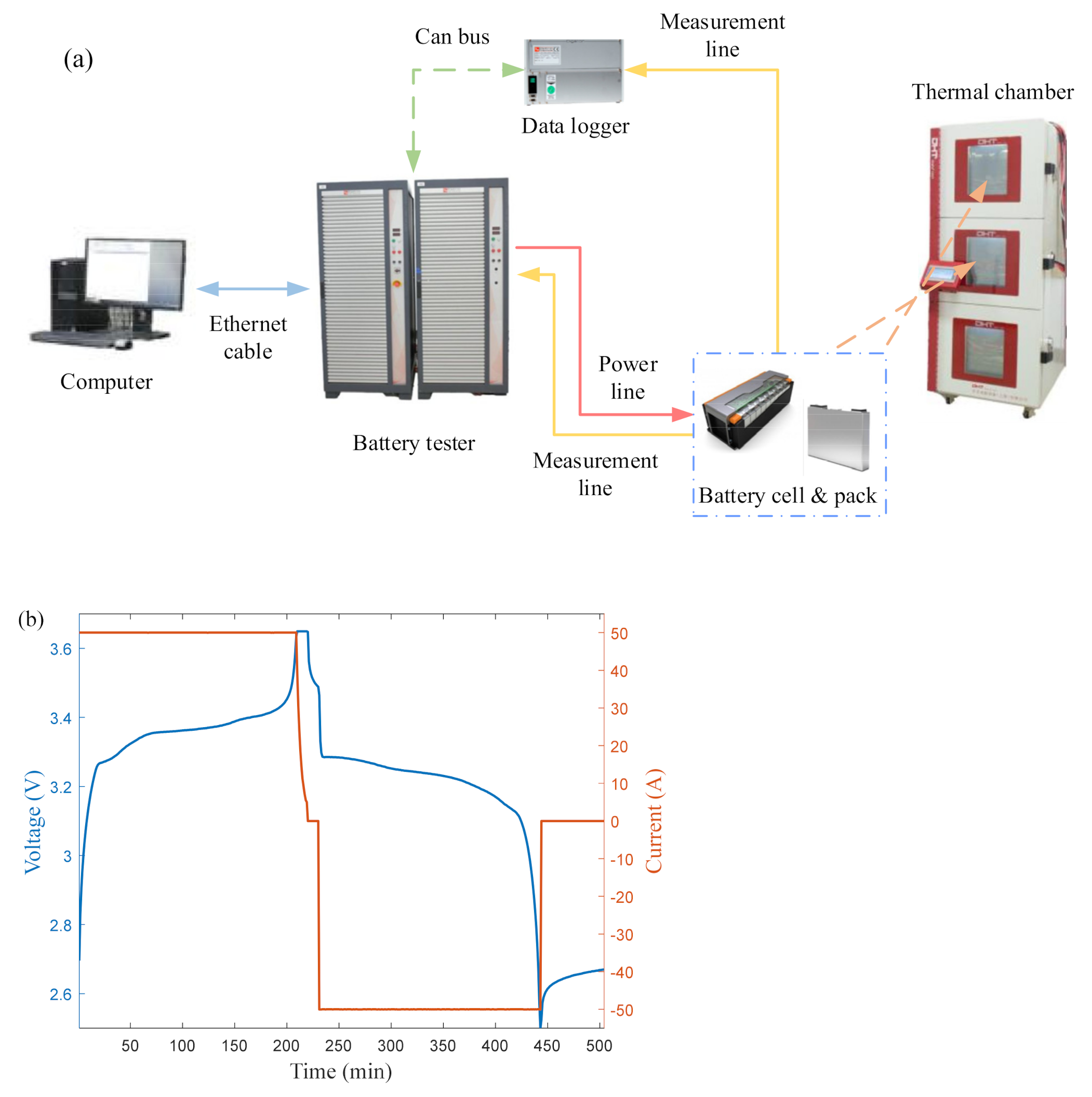
2. Aging Experiments

This section selects the battery cells under different operating conditions (sixteen battery cells divided into six groups, as shown in

Table 1. Battery and aging test parameters.

Experimental Setup Conditions	Cell #1	Cell #2	Cell #3	Cell #4	Cell #5	Cell #6	Pack
Temperature (°C)	25	25	35	35	45	55	35
Charge and discharge policies (CC-CV/CC)	0.5C/0.5C	1C/1C	0.3C/1C	0.5C/0.5C	1C/1C	1C/1C	0.5C/0.5C
Actual temperature range (°C)	25/29	25/31	35/44	36/40	45/52	54/64	36/47

) and the battery pack under the same operating conditions (35 °C_0.5C-0.5C) to complete the aging experiment. In order to analyze the effects of temperature and current on battery aging, battery cells under four different temperatures and three different currents are used for the experiments; to improve the reliability of the experiments, two or three cells are set up in the same experimental environment for each group of cells. The battery cells with a lithium iron phosphate (LiFePO₄) cathode have a 100 Ah-rated capacity. The battery pack is made up of 15 cells of the same type connected in a series (six groups). The voltage, current, time, and temperature data of the continuous cycle can be collected directly by the charge/discharge tester. The tested battery cells and battery packs are charged and discharged under constant current and constant voltage (CC-CV) conditions. The temperature of the battery pack is set to 35 °C, and the charge/discharge current is 0.5 C. Four types of temperature settings are set for the single-cell experiment: 25, 35, 45, and 55 °C. Three types of charge current settings are set: 0.3, 0.5, and 1C. Finally, two kinds of discharge current settings are set: 0.5C and 1C. The sampling time interval is 30 s for the battery pack and 10 s for the battery cells. The resting time is set to 10 min, as shown in Table 1.

The platform for the aging experiment of the battery is shown in Figure 1a, which includes a battery tester, a data logger, a thermal chamber, a computer, a series-connected battery pack, and sixteen battery cells. In the battery aging test experiment, a complete cycle of the charging and discharging process of Cell #4 is shown in Figure 1b, where the solid red line indicates the charging and discharging current. The solid blue line indicates the charging and discharging voltage. In the charging phase, the battery is first charged with a constant current (CC) of 0.5C, and when the voltage reaches the upper cutoff voltage, it switches to constant voltage (CV) charging mode until the charging current drops to 1/20 C, which ends the charging process. In the discharging stage, the battery is discharged with constant current discharge at 0.5C until the discharge voltage reaches the lower cutoff voltage; then, the discharging process is finished. The above charging and discharging steps are repeated until the battery capacity decays to 80% of its rated capacity, which marks the end of the experiment. The battery capacity aging curve is shown in Figure 2, where Figure 2a is the capacity decay curve of Cell #4 alone, and Figure 2b is the capacity decay curve of the battery pack. The battery cell offers different degrees of capacity regeneration in the decay process, among which there are three apparent fluctuations due to the long resting time. The comparison between the battery cell’s aging curve and the battery pack’s aging curve shows that the number of cycles of the pack is significantly less than the number of cycles of the battery cell when it reaches 80% SOH.

3. HI Extraction and Selection

Batteries generate large amounts of data in aging tests, and for data-driven battery health prediction methods, extracting HIs directly or indirectly from battery aging data is an essential step toward eliminating redundant data and improving computational efficiency. The extraction principle of extracting three sets of HIs from battery aging data is outlined in Section 3.1. The correlation analysis of HIs is performed by the Pearson correlation analysis method in Section 3.2.

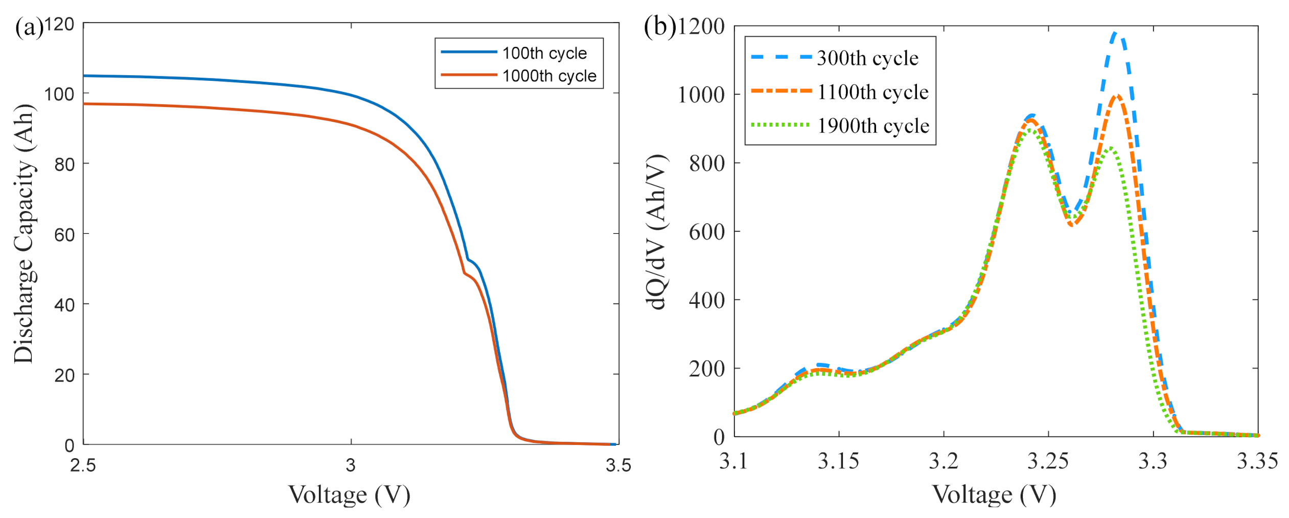
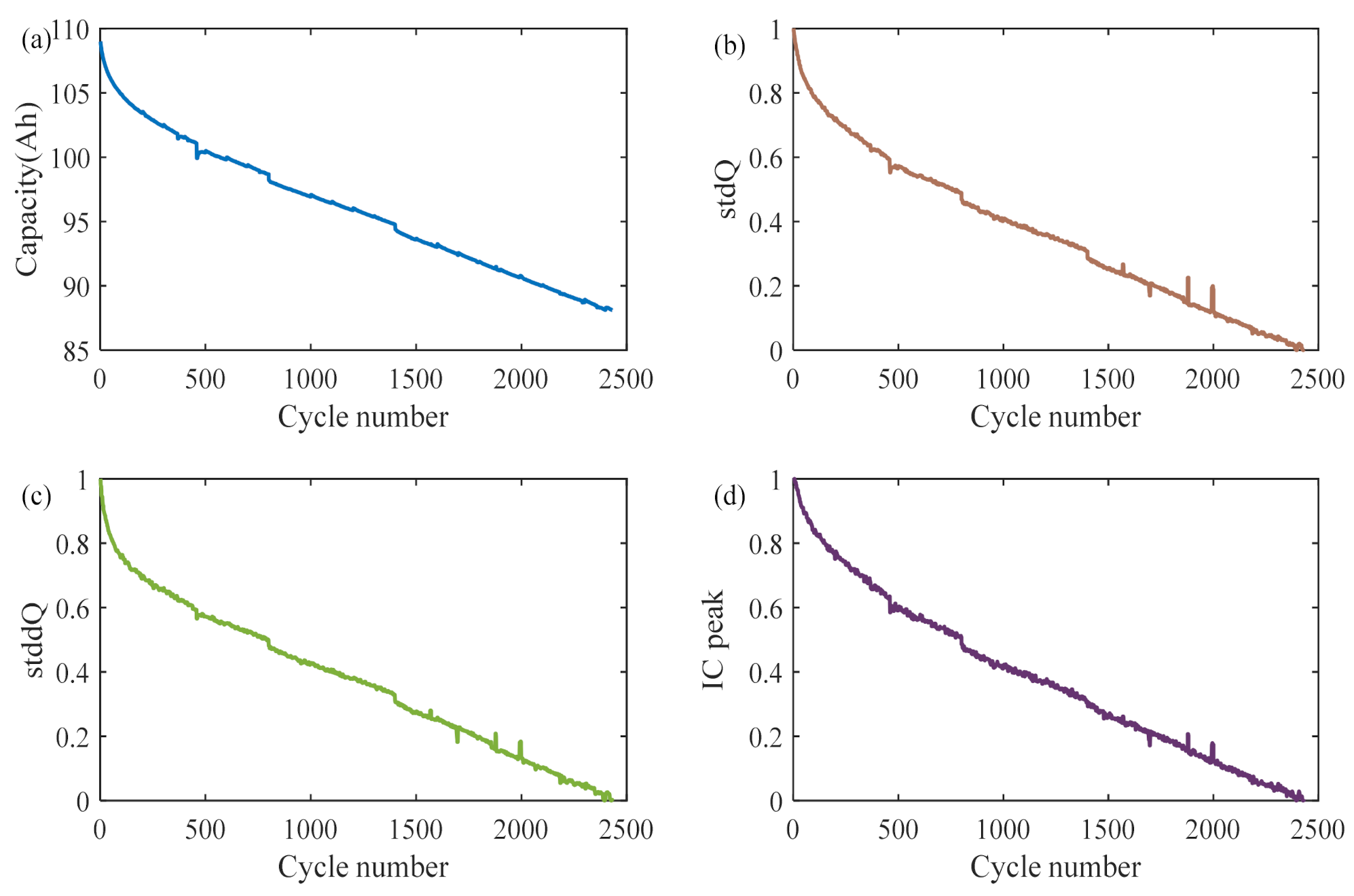
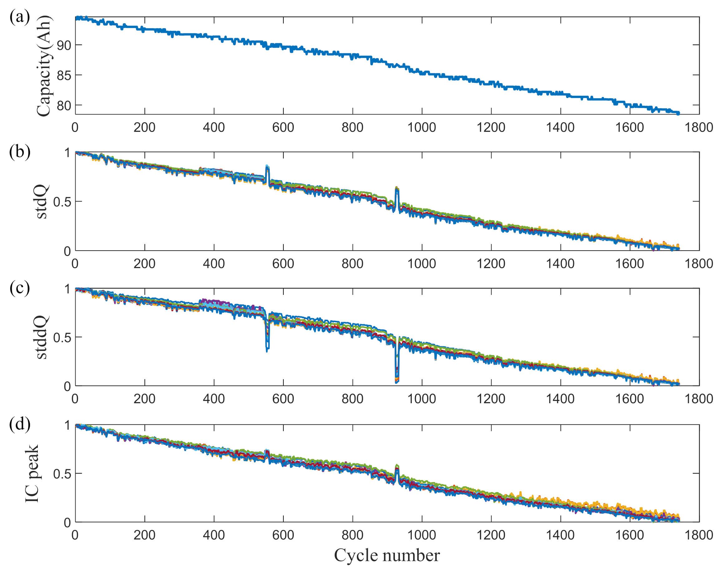
3.1. Feature Extraction

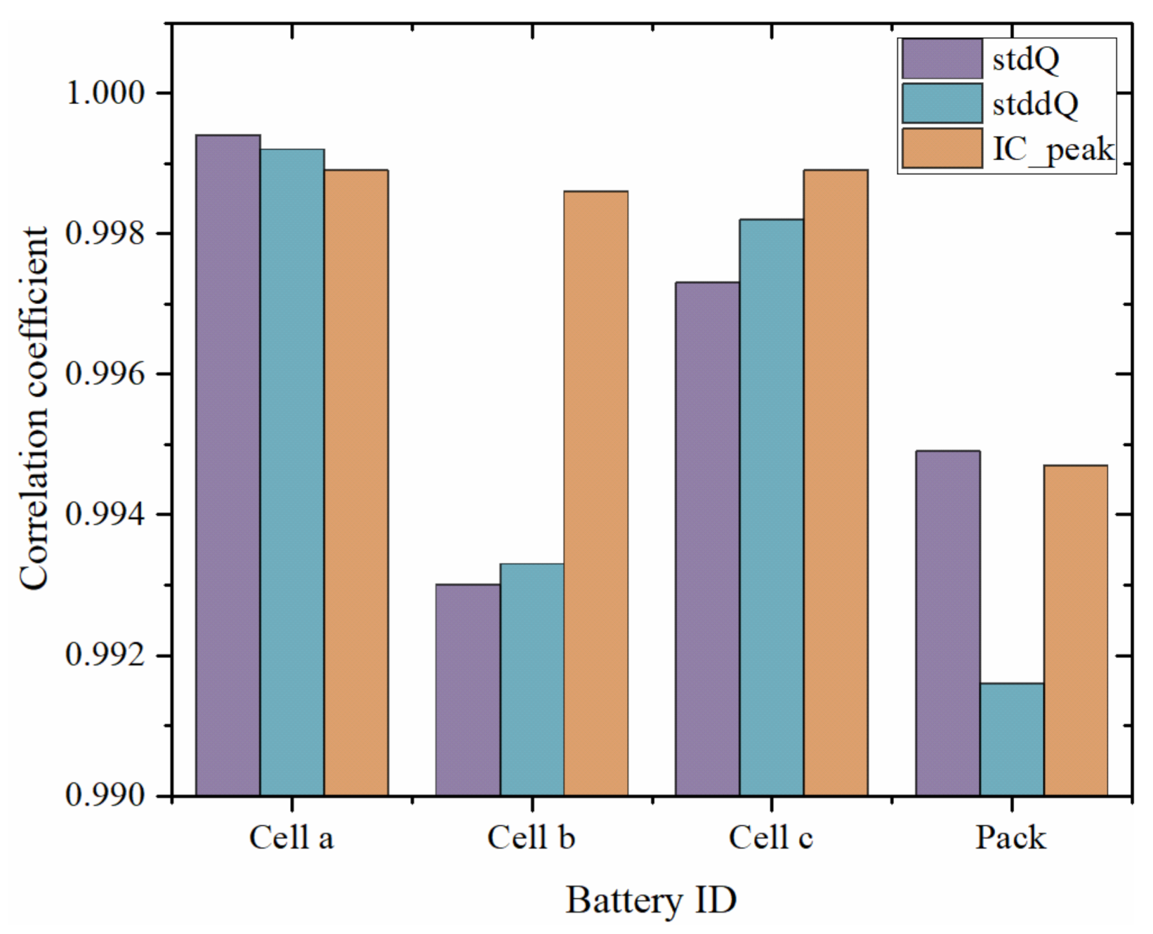
This section presents the extraction principles of the three HIs. In our previous work [24,25,26], two health factors, the standard deviation Q sequence (stdQ) and the standard deviation of different Q sequence (stddQ), have been verified to have excellent performance as the basis for the research of battery pack health prediction in this paper. The incremental capacity (IC) analysis method, as a non-destructive and effective means, has been widely used to evaluate the health status of LIBs. Since the IC_peak can capture the electrochemical processes occurring inside the battery and is closely related to the capacity decay [27], it is used as the third HI extracted in this paper.

Figure 3a represents the Q-V discharge curve of the battery under two different aging cycles (100th cycle and 1000th cycle), with the increasing number of cycles releasing the same amount of electricity at a decreasing voltage value. Firstly, a constant discharge voltage interval is selected, and the discharge voltage fragment V_seg is shown in Equation (1):

$$V_{\mathrm{seg}}=\left[V_{\max },V_{\max }-\Delta V,V_{\max }-2\ast \Delta V,\cdots ,V_{\min }\right]$$

(1)

where ΔV is the voltage interval that can be obtained through the ampere–time integration of the same voltage interval corresponding to the capacity sequence Q(v), as shown in Equation (2):

$$Q\left(V\right)=\left[Q_1,Q_2,\cdots ,Q_{N_P}\right]$$

(2)

The difference between the capacities of two different cycles can be noted as ΔQ_c2-c1(v). The standard deviation of the capacity sequence is indicated as Q(v), and the capacity sequence of different cycle differences are indicated as stdQ and stddQ, respectively.

As shown in Figure 3b, the increasing number of cycles leads to the increase in the amount of lithium ion loss inside the cell, causing the peak of the IC curve to decrease gradually. Its decay characteristics describe the aging process of the cell. The expression of the IC curve is shown in Equation (3) [20]:

$${(f^{-1})}^{\prime }=\frac{dQ}{dV}=\frac{I\cdot dt}{dV}=I\cdot \frac{dt}{dV}$$

(3)

where $V_{\min }=3.1v,V_{\max }=3.4v,N_p=50,\Delta V=6mv,dv=70mv.$

3.2. HI Selection

According to the principle of HI extraction in Section 3.1, the capacity and three sets of HI decay curves of the battery cells and battery packs can be obtained. Figure 4a shows the aging decay curve corresponding to the single cell with a rated capacity of 100 Ah. With the increasing number of cycles, the first 100 cycles show exponentially decreasing characteristics. From the 101st cycle to the end of life, the capacity showed a linear decay trend, and three capacity regeneration phenomena appeared locally. Figure 4b–d shows the decay curves of stdQ, stddQ, and IC_peak, respectively. After normalizing the extracted three groups of HIs, their decay curves are consistent with the decay curves of the monomer capacity, indicating that the proposed three groups of HIs have a closely related aging characteristic with the capacity.

Figure 5 shows the decay curves of the pack capacity and three HIs of the fifteen cells. Figure 5a shows the decay curves of the pack capacity; after the abnormal data are eliminated, the remaining capacity shows a linear monotonic decreasing trend with slight local fluctuations. In Figure 5b,c, the decay curves of stdQ and stddQ are shown, respectively. There are two apparent fluctuations and opposite directions in two cluster decay curves, indicating that anomalies occurred in two regions during the aging experiments. Figure 5d shows that IC_peak has the same aging characteristics as the capacity decay curve. Although there are two fluctuations in the same direction as the fluctuations in Figure 5b, the changes are minor.

The above analysis shows that the HIs of cells and the battery pack shows a decay characteristic consistent with the overall capacity. To further quantify the correlation degree between the HIs and the capacity, the quantitative analysis is carried out in this paper using the Pearson correlation analysis method, as shown in Equation (4) [28]:

$${\rho }_{x\mathrm{y}}=\frac{{{\displaystyle \sum }}_{i=1}^n\left(x_i-\overline{x}\right)\left(y_i-\overline{y}\right)}{\sqrt{{{\displaystyle \sum }}_{i=1}^n{\left(x_i-\overline{x}\right)}^2{{\displaystyle \sum }}_{i=1}^n{\left(y_i-\overline{y}\right)}^2}}$$

(4)

where x_i and y_i are the sample observations of x and y, respectively, and $\overline{x}$ and $\overline{y}$ are the mean of the sample values of variables x and y, respectively.

The HI correlation coefficients between cells, pack, and the corresponding capacity can be obtained from Equation (4), and the results are shown in Figure 6. As can be seen from the figure, the three sets of HIs used for the same operating condition battery cell and pack all reach 0.99. The stdQ HIs contain both battery voltage and discharge capacity curve information. The stdQ reflects the uneven battery discharge energy with the voltage, revealing the essential factors to achieve high-accuracy prediction using this feature. It indicates that the HIs strongly correlate with the battery capacity, and the extracted three sets of HIs that meet the requirements are used to establish the HI degradation model in the next stage.

4. Methodology

In this section, a method for battery pack health prognostics is proposed. A brief description of the overall prediction process is given in Section 4.1, the degradation model used to predict the future HIs of the pack is introduced in Section 4.2, and the pack health estimation model based on the GPR algorithm is presented in Section 4.3.

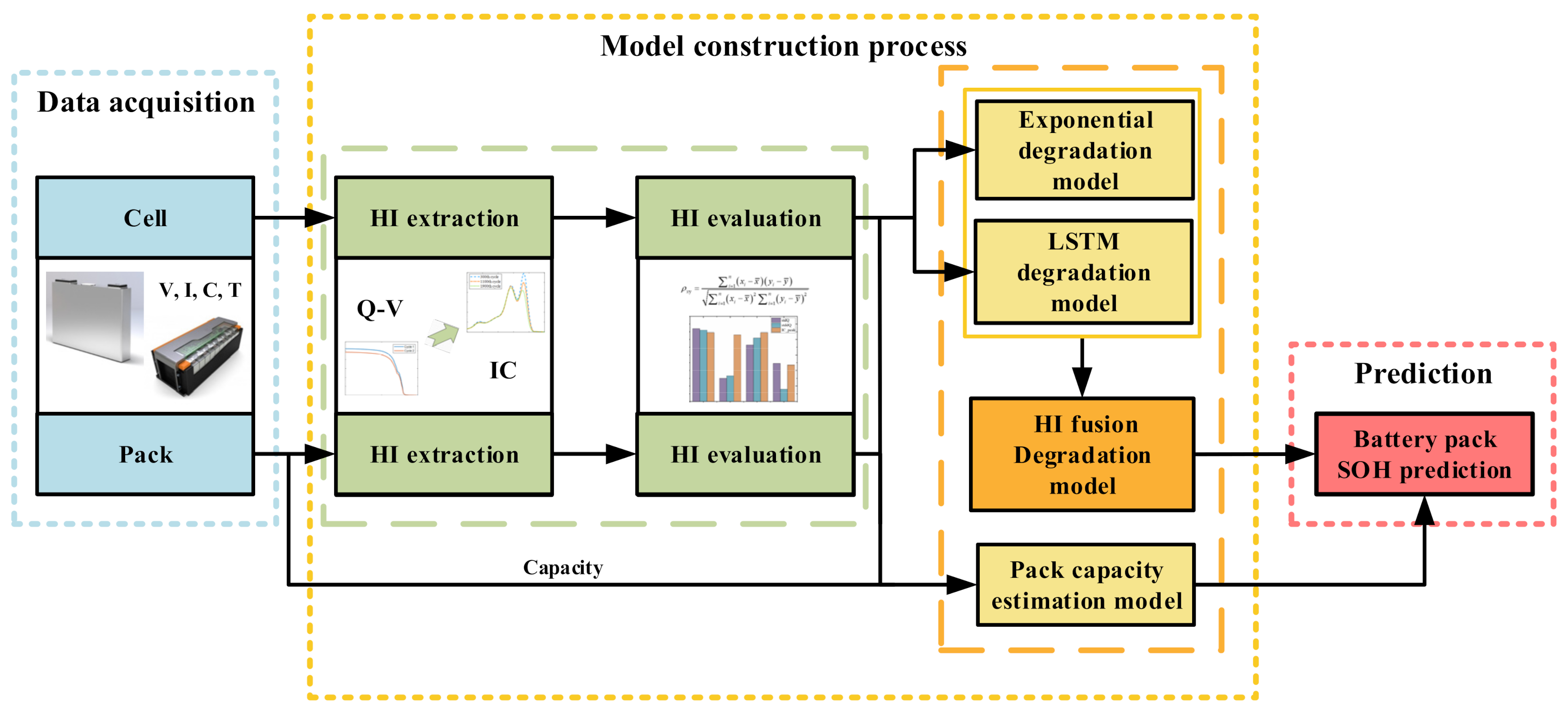
4.1. Battery Pack Health Prognostics

The proposed scheme in this paper consists of three sections, and the flowchart of the proposed scheme for battery pack health prognostics is shown in Figure 7. First section: data acquisition. First, the measured data of the battery with noise and abnormalities are pre-processed, including filling, deletion, noise reduction, smoothing, and normalization. Then, the critical data, such as voltage, current, time, etc., are screened out from the battery cells and battery pack data. Second section: the model construction process. First, three sets of HIs—stdQ, stddQ, and IC_peak—are extracted from the Q-V partial discharge curve based on the principle of HI extraction. Second, the correlation between the HIs and capacity is assessed based on the Pearson correlation analysis method. Next, the exponential degradation model and the LSTM degradation model are established based on the cell’s entire life aging data. Then, the first 10% of the battery pack HIs are used to fine-tune the above two degradation models to obtain the battery pack HI exponential degradation model and LSTM degradation model, and the two models are fused according to different weights to obtain the battery pack HI fusion degradation model. Finally, the battery pack capacity estimation model is constructed based on the GPR algorithm combined with the early battery pack HIs and capacity. Third section: battery pack health prediction. First, the predicted value of the battery pack’s future cycling HIs can be obtained by fine-tuning the HI fusion degradation model. Then, the predicted value is used as the input of the battery pack capacity estimation model, which can realize the battery pack health prediction.

4.2. HI Degradation Model

A HI fusion degradation model is proposed for predicting the HIs of the future cycles of the battery pack in this section. The main components of the fusion model are also explicitly described: the exponential (EXP) model and the long short-term memory neural network (LSTM) model.

4.2.1. EXP Model

In this section, the battery pack HI degradation model is established based on the battery pack full-life HIs through the double exponential empirical formula. The early battery pack HIs are used to realize the correction of the battery cell HI degradation model. A degradation model of battery cell HIs is established to recursively predict future cycle HIs, based on a data-driven approach to achieve the prediction of battery pack health.

By analyzing the aging characteristics of the battery, it is seen that the exponential model is closely related to the decay characteristics of the extracted HIs and can accurately track the global aging trend of the battery HIs, and the exponential model is shown in Equation (5):

$$y=a{e}^{bx}+c{e}^{dx}$$

(5)

where a, b, c, and d denote the model parameters to be determined, x is the number of battery cycles, and y is the HI.

Taking Cell #4 as an example, the HI EXP degradation model is constructed, and it includes two steps. Firstly, the model parameters are initialized as para0 = [a, b, c, d] = [0.02, −0.00701, 0.968, −0.9155 × 10⁻⁵]. Then, the updated model parameters (para1 = [a, b, c, d] = [0.024, 2.7219 × 10⁻⁴, 1.0416, −8.4452 × 10⁻⁵]) are obtained using least-squares identification to track the real degradation curve of the cell.

4.2.2. LSTM Model

LSTM is a kind of specialized recurrent neural network (RNN) for avoiding gradient vanishing and exploding problems [29]. The network structure of the LSTM, as shown in Figure 8, mainly consists of three gates and two memory states [6] (e.g., forgetting gate f_t, input gate i_t, output gate O_t, long memory C_t, and short memory h_t). The forgetting gate f_t, which is used to calculate the degree of forgetting of the information, is processed by the sigmoid function and takes a value between zero and one, where one means all retained and zero means all forgotten. The input gate i_t, used to calculate the information saved to the state unit, consists of two parts, i_t as the amount of current input information to save to the unit state, and ${\tilde{c}}_t$ as the new information generated by the current input to add to the unit state, both of which generate a new memory state. As a result, the current moment of the unit state consists of the product of the forgetting gate input and the previous moment state plus the product of the two parts of the input gate, that is, C_t. The output gate O_t is used to calculate the extent to which the information is output at the current moment. In the previous hidden state h_t−1, the current input x_t is passed to the sigmoid function. The updated cell state is passed to the tanh function, and the tanh function is multiplied with the sigmoid function output to determine the information that the hidden state should carry and what the hidden state should use as the output. Then, the new cell state and the new hidden state are transferred to the next time step, and the corresponding expression of the LSTM structure can be shown by Equation (6) [30,31,32,33]:

$$\left\{\begin{array}{l}{f}_t=\sigma \left(w_f\cdot \left[h_{t-1},x_t\right]\right)+b_f\\ i_t=\sigma \left(w_i\cdot \left[h_{t-1},x_t\right]\right)+b_i\\ {\tilde{C}}_t=\tanh \left(w_c\cdot \left[h_{t-1},x_t\right]\right)+b_c\\ C_t=f_t\ast C_{t-1}+i_t\ast {\tilde{C}}_t\\ o_t=\sigma \left(w_o\cdot \left[h_{t-1},x_t\right]\right)+b_o\\ h_t=o_t\ast \tanh \left(C_t\right)\end{array}\right.$$

(6)

where σ and tanh are the sigmoid and hyperbolic activation functions, respectively, w and b are different weight matrices and bias matrices, respectively. C_t−1 and C_t are the previous moment cell state and current cell state, respectively, and C_t is the updated cell state. h_t−1 and h_t, are the previous hidden state and the current hidden state. C_t−1, h_t−1, and x_t are the inputs of LSTM, while C_t and h_t are the outputs.

Based on the above introduction of the three gates and two memory states in the LSTM network, the HI degradation model is established as follows. Firstly, the battery cell HIs and pack HIs as inputs to the LSTM network are rearranged in the data format. Secondly, the neural network (including the LSTM network layer and the fully connected layer) is constructed, the input single-unit HIs are trained for the network, and the trained network parameters are drawn from the battery single-unit HI degradation model. Finally, the long short-term memory network is frozen, and the early cyclic HIs of separate cells in the battery pack are input into the neural network. The fully connected layer in the network is trained again, a new fully connect layer is trained, and the new neural network is the LSTM degradation model of the HIs of every single cell in the battery pack.

4.2.3. Fusion Degradation Model of HIs

Since the HI exponential degradation model only captures the global aging characteristic of the battery HIs but ignores the influence of local fluctuations on the results, it will lead to the loss of crucial information. The LSTM degradation model has the advantage of capturing local changes. However, with continuous recursion, the errors gradually accumulate, leading to too many errors to meet the accuracy requirements. To solve the problem of simultaneously capturing the global aging characteristic and local fluctuations of the HIs, a fusion degradation model in which different weights combine the exponential degradation model and the LSTM degradation model is proposed. The fusion HI degradation model (FHDM) is shown by Equation (7):

$$FHDM=\alpha \ast LSTM+(1-\alpha )\ast EXP$$

(7)

where a is the weight of the LSTM degradation model, taking values between 0 and 1. LSTM is the long short-term memory neural network degradation model, and EXP is the exponential degradation model.

4.3. GPR Algorithm

The Gaussian process regression (GPR) algorithm is a machine learning method based on Bayesian theory. The advantages of being flexible, nonparametric, and able to integrate uncertainty expressions are widely valued in battery health prediction. This section provides a brief introduction to the GPR algorithm [34].

A formula for any GPR problem is shown in Equation (8):

$$\mathrm{y}=f(x)+\epsilon ·\epsilon \sim N(0,{\sigma }^2)$$

(8)

where y is the observed value containing the noise, ε is a Gaussian white noise that satisfies the mean value of zero, and f(x) is a function that obeys the Gaussian probability distribution, as shown in Equation (9):

$$f(x)\sim GP(m(x),k_f(x,x\prime ))$$

(9)

where m(x) is the mean function, usually taken to zero, k_f is the kernel function, used to characterize the distance or similarity between the two points of the input quantity, and the commonly used covariance function is the squared exponential (SE) covariance function, as shown in Equation (10) [35]:

$$K_f={\sigma }_f^2\exp (-\frac{1}{2}(x-x\prime )l^{-1}(x-x\prime ))$$

(10)

where the signal covariance ${\sigma }_f^2$ is the output amplitude and l is the characteristic length scale.

For the observed value y that obeys a Gaussian distribution and considers Gaussian white noise, the prior distribution is as shown in Equation (11):

$$y\sim N(0,K_f(X,X)+{\sigma }_n^2{I}_n)$$

(11)

The set of parameters $\Theta =\left[{\sigma }_f,l,{\sigma }_n\right]$ in Equation (10) is the hyper-parameter, and the optimal solution of the hyper-parameter is obtained by establishing the negative logarithmic marginal likelihood function negative logarithmic marginal likelihood (NLML) to find the partial derivatives of the hyper-parameter, and then using the conjugate gradient method to minimize the partial derivatives, as shown in Equation (12):

$$L=logp(y|X,\Theta )=-\frac{1}{2}{y}^T{[K_f(X,X)+{\sigma }_n^2{I}_n]}^{-1}y-\frac{1}{2}log(det(K_f(X,X)+{\sigma }_n^2{I}_n))-\frac{nlog2\pi }{2}$$

(12)

The joint Gaussian distribution of the observed value y and the predicted value y* is shown in Equation (13):

$$\left[\begin{array}{c}y\\ y^{*}\end{array}\right]\sim N\left(0,\left[\begin{array}{cc}(K_f(X,X)+{\sigma }_n^2{I}_n& K_f(X,X^{*})\\ K_f{(X,X^{*})}^T& K_f(X^{*},X^{*})\end{array}\right]\right)$$

(13)

According to Bayesian theory, the posterior distribution is as shown in Equation (14):

$$p\left(y^{*}|X,y,X^{*}\right)=N\left(y^{*}|{\overline{y}}^{*},{\sigma }^2(y^{*})\right)$$

(14)

where ${\overline{y}}^{*}$ is the predicted mean, and ${\sigma }^2(y^{*})$ is the predicted covariance, as given in Equation (15):

$$\left\{\begin{array}{c}{\overline{y}}^{*}=K_f{(X,X^{*})}^T{[K_f(X,X)+{\sigma }_n^2{I}_n]}^{-1}y\\ {\sigma }^2(y^{*})=K_f(X^{*},X^{*})-K_f{(X,X^{*})}^T{[K_f(X,X)+{\sigma }_n^2{I}_n]}^{-1}{K}_f(X,X^{*}))\end{array}\right.$$

(15)

To quantitatively evaluate the actual effect of the proposed scheme, three indicators—the 95% confidence interval (95% CI), the mean absolute error (MAE), and the root mean square error (RMSE)—are used to evaluate the prediction performance of the GPR algorithm, as shown in Equation (16):

$$\left\{\begin{array}{l}95\%\mathrm{CI}={\overline{y}}^{\ast }\mp 1.96\times \sigma (y^{\ast })\\ RMSE=\sqrt{\frac{1}{N}{\displaystyle {\sum }_{i=1}^N{(y_i-{\overline{y}}_i^{*})}^2}}\\ MAE=\frac{1}{N}{\displaystyle {\sum }_{i=1}^N|y_i-{\overline{y}}_i^{*}|}\end{array}\right.$$

(16)

where 95%CI is the confidence interval, ${\overline{y}}^{\ast }$ and $y^{\ast }$ are the predicted value and variance, respectively. N is the size of the testing set, y_i is the actual value, and ${\overline{y}}_i^{*}$ is the estimated value.

5. Results and Discussion

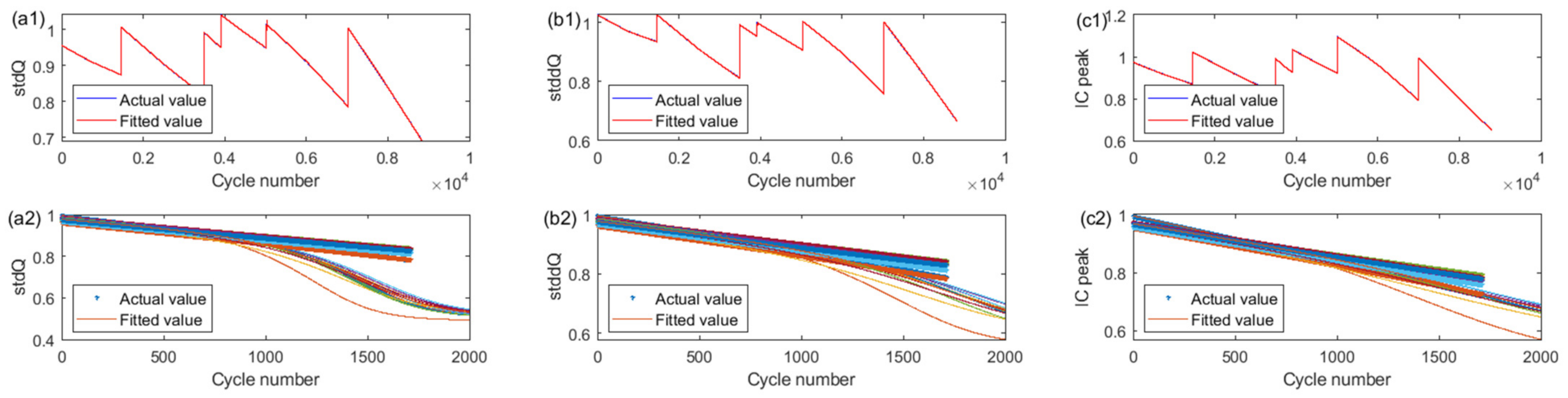
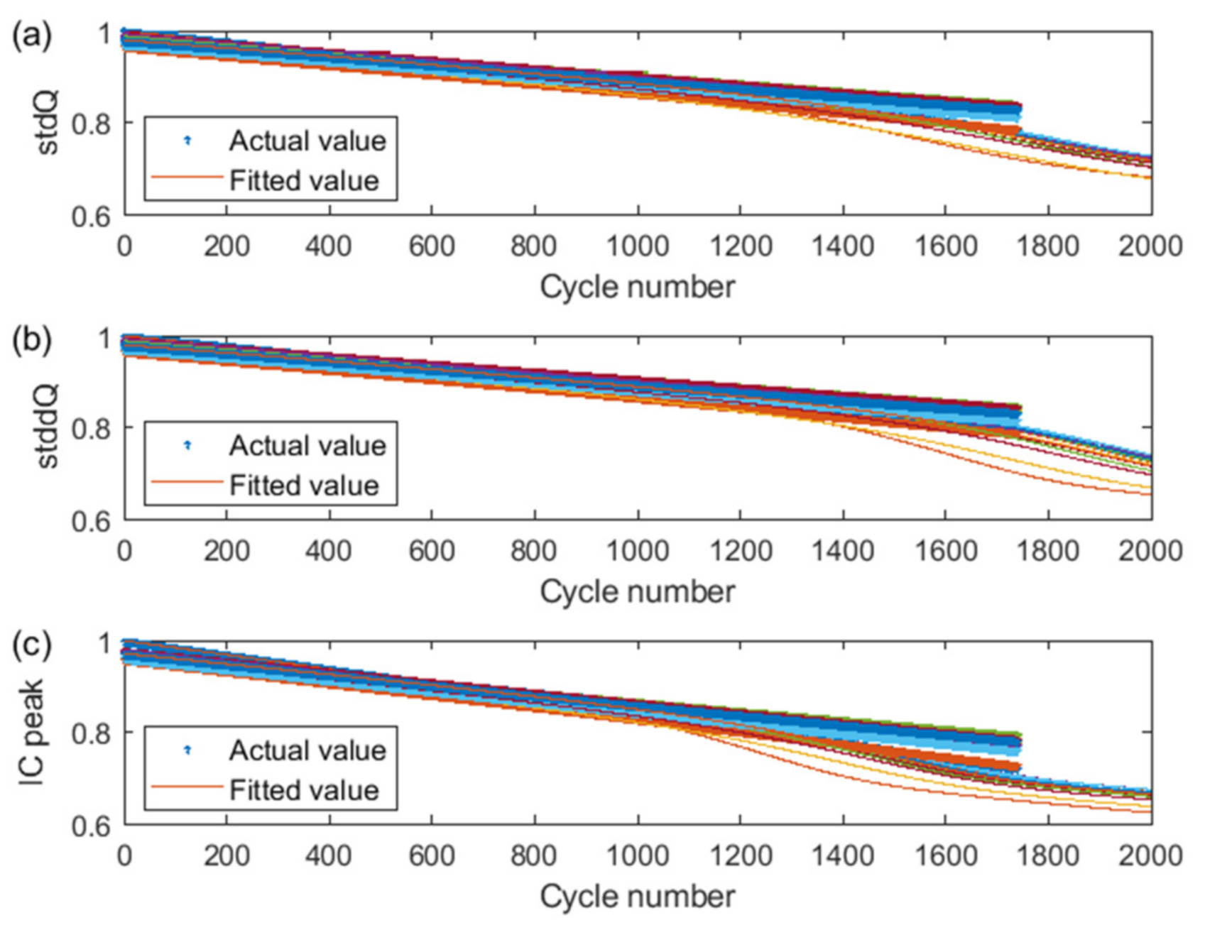
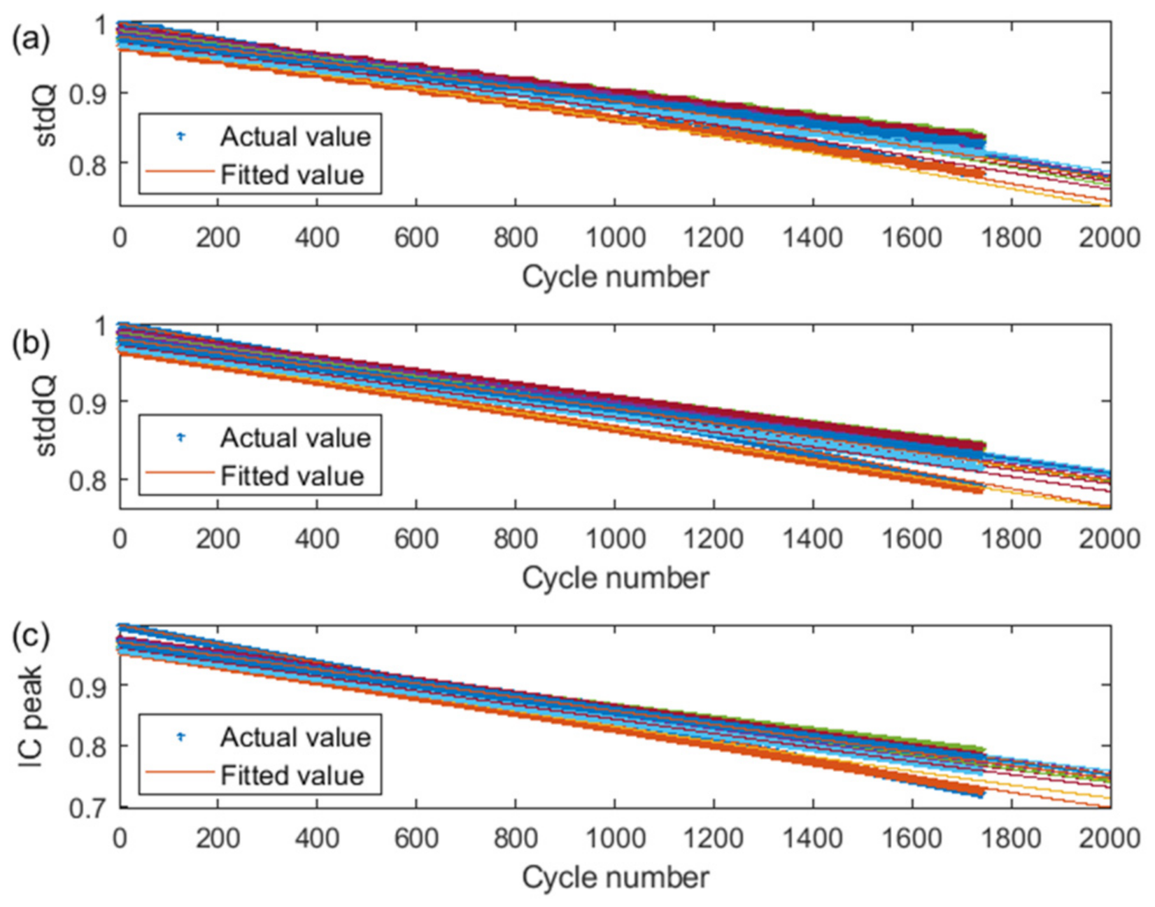
In this section, the experimental aging data are used to evaluate battery pack health prognosis methods. The single degradation and fused degradation models are validated based on the HIs by using the experimental data of battery aging under the same and different operating conditions in Section 5.1. The effect of the battery pack’s health prediction model is verified by the future cycling the HIs predicted by the single degradation model and the fused degradation model, and the prediction results are quantitatively analyzed and discussed in Section 5.2.

5.1. HI Prediction

This section describes two types of HI degradation models: the single degradation models (the EXP degradation model and the LSTM degradation model) and the fusion degradation model. Firstly, the prediction accuracy of the single degradation model is verified by using three sets of HIs under the same and different operating conditions, and the applicability range of each single degradation model is compared. Secondly, the prediction accuracy of the fusion degradation model is verified using the HIs under the same condition and the different operating conditions, and the results are analyzed and discussed accordingly.

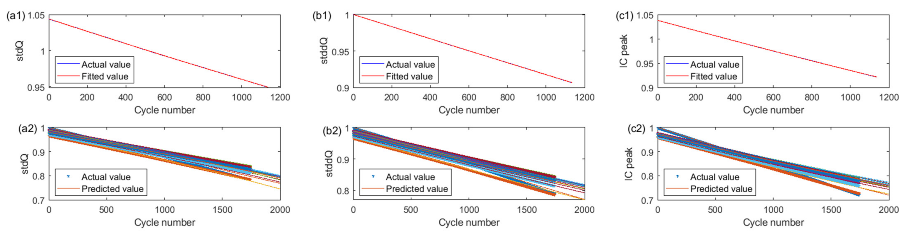
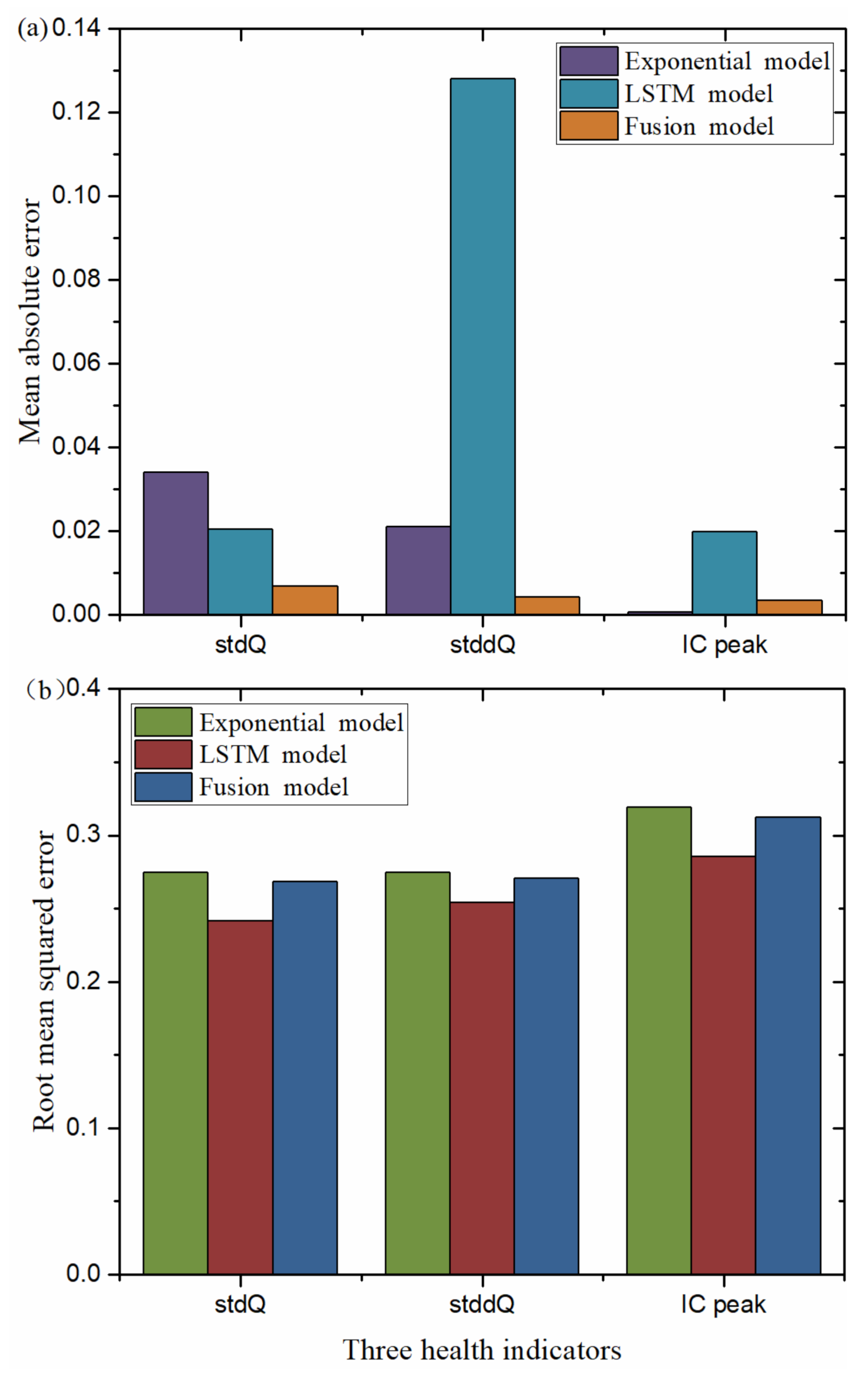
5.1.1. Single Degradation Model

The single degradation model includes the EXP degradation model and the LSTM degradation model. For the EXP degradation model under the same operating condition (charge and discharge current is 0.5C and temperature is 35 °C), the corresponding decay curves before and after the correction of the HI degradation model for Cell #4 under the same operating condition are shown in Figure 9. Figure 9(a1,b1,c1) shows the decay curves of the three HIs of Cell #4 under the same operating condition (before correction), where the blue line is the actual value and the red line is the estimated value of the EXP degradation model based on the least-squares method. Using the battery pack early 10% HIs to correct the HI EXP degradation model, the model of the battery pack corresponding to the three sets of HI decay curves (after correction) are shown in Figure 9(a2,b2,c2), where the dotted line is the actual value and the solid line is the fitted value. The MAE and RMSE between the actual values and the predicted values for the EXP degradation model of the battery pack under the same operating condition are 0.034, 0.021, 0.006, and 0.2745, 0.2746, 0.3191, respectively. The aging characteristic of individual HIs in the battery pack is in good agreement with the global aging characteristic of the predicted values, indicating that the EXP degradation model can capture the global HI decay tendency with high accuracy, but cannot capture the local HI variation trend.

For the LSTM degradation model under the same operating condition, the three sets of the HI decay curves corresponding to Cell #4 with the fitted curves are shown in Figure 10(a1,b1,c1) (before correction), where the blue line is the actual value and the red line is the predicted value of the LSTM degradation model. Figure 10(a2,b2,c2) shows the decay curves of the three HIs corresponding to the battery pack with the predicted values (after correction). Due to the gradual accumulation of errors in the recursive rolling process of the LSTM model, although the deviation of the predicted values from the actual values is slight for the first 900 cycles, the errors increase rapidly from the 901st cycle to the 1742nd cycle as the cycles continue to accumulate. Then, the LSTM degradation model experiences the error accumulation effect under the same operating condition, and the error is too large to correct at the later stage. The MAE and RMSE between the actual values and the predicted values for the LSTM degradation model of the battery pack under the same operating condition are 0.0523, 0.0401, 0.11 and 0.1624, 0.1933, 0.0939, respectively. The results show that the local aging characteristics of the pack HIs are in good agreement with the predicted values, indicating that the LSTM degradation model can capture the ageing characteristic of local HIs. Nevertheless, the ability to capture the aging characteristic of global HIs is relatively poor due to the disadvantages of cumulative errors.

For the LSTM degradation model under the different operating conditions, the corresponding three sets of HI aging curves and fitted curves (before correction) for six groups of battery cells under different operating conditions are shown in Figure 11(a1,b1,c1), where the blue line is the actual value and the red line is the predicted value of the LSTM degradation model. The three sets of HI decay curves of the battery pack are shown in Figure 11(a2,b2,c2), where the dotted line is the actual decay curve and the solid line is the LSTM degradation model prediction curve (after correction). Compared with the same condition decay curves in Figure 10(a2,b2,c2), the corresponding prediction accuracy of the LSTM degradation model prediction values under the different operating conditions is improved, where the improvement of stddQ and IC_peak is prominent. The MAE and RMSE between actual values and the predicted values for the LSTM degradation model of the battery pack under the different operating conditions are 0.0203, 0.128, 0.197 and 0.2417, 0.2543, 0.2855, respectively. By comparing this with the LSTM degradation model under the same operating condition, the result shows that the consistent local and global aging characteristics of the pack HI aging trends with the predicted values are significantly improved. The results indicate that the type, quantity, and quality of the battery aging data under the different operating conditions play crucial roles in enhancing the ability of the LSTM degradation model to capture the local and global HI aging trends.

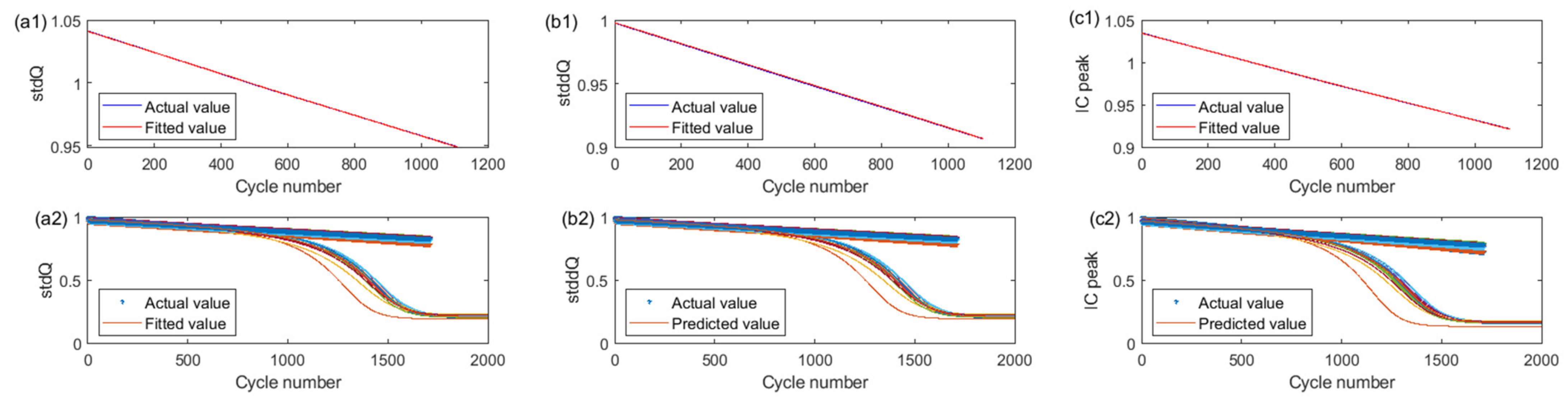
5.1.2. Fusion Degradation Model

The single HI EXP degradation model cannot capture the local variation of the HI decay characteristics. In contrast, the single HI LSTM degradation model cannot capture the global variation of the HI decay characteristics. The battery aging data of the same and different operating conditions are used here to verify the proposed fusion degradation model to solve the above shortcomings.

The actual decay curves and the predicted decay curves are based on the fusion degradation model for the three HIs of the battery pack under the same operating condition, as shown in Figure 12a–c. The dotted lines are the actual values of the HIs, and the solid lines are the predicted values of the HIs. The MAE and RMSE of the three HIs of the battery pack are 0.0132, 0.0097, 0.0215 and 0.256, 0.2604, 0.2823, respectively. The overall accuracy of MAE and RMSE of the fusion degradation model is better than the single HI EXP degradation model. However, the predicted value of IC_peak is much lower than the single HI EXP degradation model. The MAE of the fusion degradation model is better than the LSTM degradation model. The RMSE is between the predicted values of the single EXP degradation model and the predicted values of the single LSTM degradation model.

The decay curves of the three sets of HIs and the predicted decay curves based on the fusion model are shown in Figure 13a–c, where the dotted lines are the actual values of the HIs and the solid lines are the predicted values of the HIs under the different operating conditions. The MAE and RMSE of the fusion degradation model for the three sets of HIs are 0.0068, 0.042, 0.0034 and 0.2682, 0.2707, 0.3126, respectively. The results show that the fusion degradation model under the different operating conditions has better accuracy and ability to capture the HIs than the single HI EXP degradation model and single LSTM degradation model.

The prediction accuracies correspond to the single degradation model and the fused degradation model under the different operating conditions, as shown in Figure 14. Figure 14a represents the mean absolute error (MAE) corresponding to the three HIs under different degradation models. By comparing the MAE under the three degradation models, the results show that the prediction accuracy of the fusion degradation model is higher than that of the exponential degradation model and the LSTM degradation model, in which the stdQ and stddQ accuracy of the single degradation models (EXP degradation model and LSTM degradation model) are substantially improved. Figure 14b represents the root mean square error (RMSE) corresponding to the three HIs under different degradation models. The RMSE corresponding to the three sets of HIs of the fusion degradation model has errors between the exponential degradation model and the LSTM degradation model. The results show that the fusion degradation model can capture the global aging trend of the HIs in the EXP degradation model and eliminate the shortcoming of excessive cumulative errors in the recursive process of the LSTM degradation model, and thus has satisfactory estimation accuracy.

5.2. Battery Pack SOH Prediction

In this section, the prediction accuracy of the battery pack health prediction method is verified based on the predicted value of the HI fusion decay model under the same operating condition and the different operating conditions, combined with the battery pack capacity estimation model. Among them, the same operating condition means that both battery cells and the battery pack work at 35 °C_0.5C-0.5C; different operating conditions mean that battery cells work in six different environments (see Table 1 for details) and battery pack works at 35 °C_0.5C-0.5C.

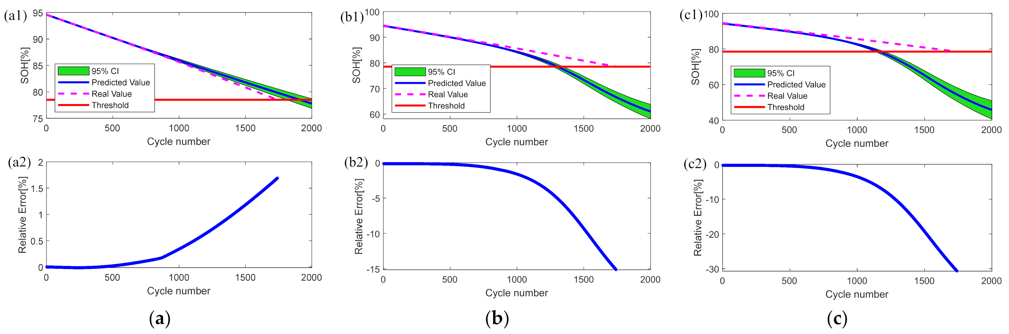
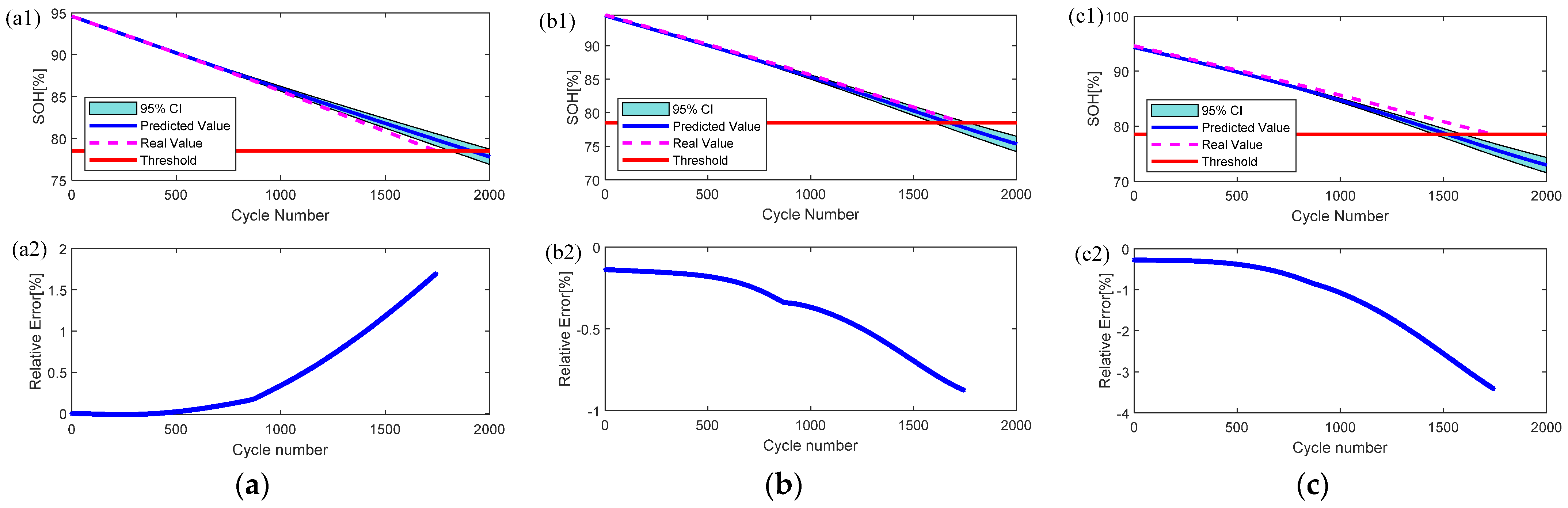
5.2.1. Prediction Results Using the Same Operating Condition

Under the same operating condition, the battery pack cycle life early 10% HIs and capacity are used as the training set of the battery pack capacity estimation model. On the basis of the EXP degradation model, the LSTM degradation model, and the fusion degradation model, used to predict the future HIs of the battery pack, the predicted battery pack state of health is analyzed against the actual value to calculate the error. Figure 15 shows the corresponding battery pack state of health prediction results under the three groups of models: the HI exponential degradation model-GPR capacity prediction model (EXP-GPR), the HI exponential degradation model–HI LSTM degradation model–GPR capacity prediction model (EXP-LSTM-GPR), and the HI LSTM degradation model–GPR capacity prediction model (LSTM-GPR). Figure 15(a1,b1,c1) shows the prediction error of the battery pack for each of the three cases. The solid red line indicates the battery state of the health cutoff threshold. The red dotted line is the actual value, the solid blue line is the estimated value, and the green shaded area is the 95% confidence interval used to describe the uncertainty of the prediction result. Figure 15(a2,b2,c2) shows the relative errors under the three groups of models EXP-GPR, EXP-LSTM-GPR, and LSTM-GPR, respectively. Among them, Figure 15(a2) shows that the relative error corresponding to the first 406 cycles is negative, while the relative error from the 407th cycle to the 850th cycle is positive and exponentially increasing. Then, the error increases rapidly from the 851st cycle to the 1742nd cycle, and the maximum relative error is only 1.7%. Figure 15(b2) indicates that the relative errors of the fusion model are all negative when the weights of the single degradation model are 0.5. The relative error is less than −0.4% for the first 600 cycles, and the relative error shows exponential growth from the 601st cycle to the 1200th cycle. The error increases linearly and rapidly from the 1201st cycle, with the maximum relative error reaching −15%. Comparing Figure 15c with Figure 15b, the result shows that the two relative errors have the same trend, but the maximum relative error of the latter is about twice as large as that of the former.

Under the same operating condition, the EXP degradation model and LSTM degradation model are fused based on different weights, and the HI fusion degradation model thus predicts the future cycle HIs of the battery pack, which is combined with the battery pack capacity estimation model to achieve a state of health prediction. The errors under the different weights are shown in Figure 16, where the horizontal coordinates indicate the weight of the LSTM degradation model in the fusion model and the vertical coordinates indicate the corresponding errors under different weights. The results show that the fusion degradation model can track the capacity regeneration phenomenon with different degrees of accuracy due to its inability to cover the range of parameter variation within the battery pack. The prediction accuracy based on the battery pack health state prediction model needs to be optimized.

5.2.2. Prediction Results Using the Different Operating Conditions

Under the different operating conditions, using the HI degradation model to predict the future HIs, the prediction results will verify the prediction accuracy of the battery pack capacity estimation model and the corresponding prediction results and relative errors, as shown in Figure 17. Figure 17a shows the fusion degradation model under the different operating conditions and the LSTM degradation model with a weight coefficient of zero predicted for the battery pack. The relative error of the early cycle is negative, the relative error of the mid-cycles is positive and shows an exponential growth trend, and the relative error of the later cycle increases rapidly, while the maximum relative error is only 1.7%. Figure 17c shows that the predicted value is consistently smaller than the actual value as the number of cycles increases. The relative error is less than −0.5% and remains stable for the first 600 cycles and increases linearly and rapidly from the 601st cycle to the 1742nd cycle, with the maximum relative error being less than −4%. Compared with Figure 17a,c, Figure 17b shows the prediction HIs of the fusion model when the weights of the single degradation model are 0.5, and the SOH prediction accuracy based on the fusion degradation model is higher than the others. The first 880 cycles are stable within −0.35%, and the error gradually increases after the 880th cycle, with a maximum relative error of 0.87%.

Under the different operating conditions, the EXP degradation model and the LSTM degradation model are constructed as fusion models with different weights to predict the future cycle HIs of the battery pack, and the battery pack capacity estimation model is validated based on the predicted HIs. The errors correspond to the different weights of the fusion degradation model, as shown in Figure 18, where the horizontal coordinates indicate the weights of the LSTM degradation model in the fusion degradation model, and the vertical coordinates indicate the errors corresponding to the different weights. With the increasing weight of the LSTM model, both MAE and RMSE show a ‘V’ shape, and both errors of MAE and RMSE reach the maximum when the LSTM degradation model is adopted separately. The highest prediction accuracy is obtained by fusing the EXP degradation model and the LSTM degradation model with 0.7 and 0.3 weights under the different operating conditions, and the corresponding MAE and RMSE are 7.17% and 7.81%, respectively. The results show that the fused degradation model can achieve satisfactory prediction accuracy when combined with the battery pack capacity estimation model for SOH prediction.

6. Conclusions

This paper proposes a new method to predict the health of a battery pack based on its early cycling data and the complete aging data of battery cells. Firstly, three sets of HIs are extracted from the experimental data of battery cells and the battery pack. The correlations between the HIs and capacity are verified by the Pearson correlation analysis method. The results show that their correlation coefficients are greater than 0.99, indicating the HIs are highly related to the battery capacity. To predict the future HIs of battery cells, an exponential degradation model is fitted to capture the global decay of HIs, while a LSTM degradation model is constructed to imitate the local variation of HIs. A fusion degradation model can be created by weighting the exponential-based model and LSTM-based model, which can inherit the advantages of these two models. Then, an early prognosis method for battery pack health is proposed. Based on the early cycling data of the battery pack and the fusion degradation model of HIs, the future HIs of the battery pack can be obtained. Taking the HIs as the inputs of the GPR algorithm, data-driven models can be constructed to predict the future health of the battery pack. Finally, three health prediction models based on the GPR algorithm are constructed for comparison, including the exponential function-based (EXP-GPR) model, LSTM-based (LSTM-GPR) model, and their weighted fusion-based (EXP-LSTM-GPR) model. A comparison of the errors of the three different models for two different operating conditions is shown in

Table 2. Comparison of the errors of different models under different working conditions.

Operating Conditions	Accuracy	Model
		EXP-GPR	LSTM-GPR	EXP-LSTM-GPR
Same operating conditions	MAE (%)	0.3681	7.6437	2.1477
	RMSE (%)	0.5517	12.0944	3.4502
Different operating conditions	MAE (%)	0.3681	0.9951	0.0717
	RMSE (%)	0.5517	1.2476	0.0781

. The results show that the fused degradation model has better accuracy under the different operating conditions, and its MAE and RMSE are 7.17% and 7.81%, respectively.

The method proposed in this paper is of excellent engineering utility for the rapid development of battery packs and for evaluating their performance indexes. It can save more than 50% of the aging experiment time and labor costs, make full use of the existing test data to predict the life of unknown battery cells and packs, and facilitate the development and selection cycle. The whole-lifecycle prediction is completed by using the data of a small number of cycles, which can improve the accuracy of the life prediction of battery cells and battery packs and broaden the application scope to solve the problem of life prediction under different temperatures, different currents, and different cell models. However, the proposed scheme in this paper only validates the same type of battery cells and battery packs. This method can be applied to different types of batteries and capacity diving problems within the scope of principle analysis, but further validation is needed, which is also our next problem to solve.

References

1. Hu, X.; Xu, L.; Lin, X.; Pecht, M. Battery Lifetime Prognostics. Joule 2020, 4, 310–346. [Google Scholar] [CrossRef]
2. Severson, K.A.; Attia, P.M.; Jin, N.; Perkins, N.; Jiang, B.; Yang, Z.; Chen, M.H.; Aykol, M.; Herring, P.K.; Fraggedakis, D.; et al. Data-driven prediction of battery cycle life before capacity degradation. Nat. Energy 2019, 4, 383–391. [Google Scholar] [CrossRef] [Green Version]
3. Deng, Z.; Hu, X.; Lin, X.; Kim, Y.; Li, J. Sensitivity Analysis and Joint Estimation of Parameters and States for All-Solid-State Batteries. IEEE Trans. Transp. Electrif. 2021, 7, 1314–1323. [Google Scholar] [CrossRef]
4. Zhang, Y.; Wang, C.-Y.; Tang, X. Cycling degradation of an automotive LiFePO4 lithium-ion battery. J. Power Sources 2011, 196, 1513–1520. [Google Scholar] [CrossRef]
5. Shu, X.; Shen, S.; Shen, J.; Zhang, Y.; Li, G.; Chen, Z.; Liu, Y. State of health prediction of lithium-ion batteries based on machine learning: Advances and perspectives. iScience 2021, 24, 103265. [Google Scholar] [CrossRef]
6. Li, W.; Sengupta, N.; Dechent, P.; Howey, D.; Annaswamy, A.; Sauer, D.U. Online capacity estimation of lithium-ion batteries with deep long short-term memory networks. J. Power Sources 2021, 482, 228863. [Google Scholar] [CrossRef]
7. Yang, S.; Zhang, C.; Jiang, J.; Zhang, W.; Zhang, L.; Wang, Y. Review on state-of-health of lithium-ion batteries: Characterizations, estimations and applications. J. Clean. Prod. 2021, 314, 128015. [Google Scholar] [CrossRef]
8. Li, Y.; Liu, K.; Foley, A.; Zülke, A.; Berecibar, M.; Nanini-Maury, E.; Van Mierlo, J.; Hoster, H.E. Data-driven health estimation and lifetime prediction of lithium-ion batteries: A review. Renew. Sustain. Energy Rev. 2019, 113, 109254. [Google Scholar] [CrossRef]
9. Ge, M.-F.; Liu, Y.; Jiang, X.; Liu, J. A review on state of health estimations and remaining useful life prognostics of lithium-ion batteries. Measurement 2021, 174, 109057. [Google Scholar] [CrossRef]
10. Schmalstieg, J.; Käbitz, S.; Ecker, M.; Sauer, D.U. A holistic aging model for Li (NiMnCo) O2 based 18650 lithium-ion batteries. J. Power Sources 2014, 257, 325–334. [Google Scholar] [CrossRef]
11. Hu, X.; Li, S.; Peng, H. A comparative study of equivalent circuit models for Li-ion batteries. J. Power Sources 2012, 198, 359–367. [Google Scholar] [CrossRef]
12. Lai, X.; Gao, W.; Zheng, Y.; Ouyang, M.; Li, J.; Han, X.; Zhou, L. A comparative study of global optimization methods for parameter identification of different equivalent circuit models for Li-ion batteries. Electrochim. Acta 2019, 295, 1057–1066. [Google Scholar] [CrossRef]
13. Hu, X.; Yuan, H.; Zou, C.; Li, Z.; Zhang, L. Co-Estimation of State of Charge and State of Health for Lithium-Ion Batteries Based on Fractional-Order Calculus. IEEE Trans. Veh. Technol. 2018, 67, 10319–10329. [Google Scholar] [CrossRef]
14. Jokar, A.; Rajabloo, B.; Désilets, M.; Lacroix, M. Review of simplified Pseudo-two-Dimensional models of lithium-ion batteries. J. Power Sources 2016, 327, 44–55. [Google Scholar] [CrossRef]
15. Galeotti, M.; Cinà, L.; Giammanco, C.; Cordiner, S.; Di Carlo, A. Performance analysis and SOH (state of health) evaluation of lithium polymer batteries through electrochemical impedance spectroscopy. Energy 2015, 89, 678–686. [Google Scholar] [CrossRef]
16. Xu, L.; Lin, X.; Xie, Y.; Hu, X. Enabling high-fidelity electrochemical P2D modeling of lithium-ion batteries via fast and non-destructive parameter identification. Energy Storage Mater. 2021, 45, 952–968. [Google Scholar] [CrossRef]
17. Lipu, M.S.H.; Hannan, M.; Hussain, A.; Hoque, M.; Ker, P.J.; Saad, M.; Ayob, A. A review of state of health and remaining useful life estimation methods for lithium-ion battery in electric vehicles: Challenges and recommendations. J. Clean. Prod. 2018, 205, 115–133. [Google Scholar] [CrossRef]
18. Klass, V.; Behm, M.; Lindbergh, G. A support vector machine-based state-of-health estimation method for lithium-ion batteries under electric vehicle operation. J. Power Sources 2014, 270, 262–272. [Google Scholar] [CrossRef]
19. Li, H.; Pan, D.; Chen, C.L.P. Intelligent Prognostics for Battery Health Monitoring Using the Mean Entropy and Relevance Vector Machine. IEEE Trans. Syst. Man Cybern. Syst. 2014, 44, 851–862. [Google Scholar] [CrossRef]
20. Li, X.; Wang, Z.; Yan, J. Prognostic health condition for lithium battery using the partial incremental capacity and Gaussian process regression. J. Power Sources 2019, 421, 56–67. [Google Scholar] [CrossRef]
21. Che, Y.; Deng, Z.; Hu, X. Battery pack state of health estimation with general health indicators and modified gaussian process regression. In Proceedings of the 34th International Electric Vehicle Symposium and Exhibition (EVS34), Nanjing, China, 25–28 June 2021. [Google Scholar]
22. Deng, Z.; Hu, X.; Li, P.; Lin, X.; Bian, X. Data-Driven Battery State of Health Estimation Based on Random Partial Charging Data. IEEE Trans. Power Electron. 2021, 37, 5021–5031. [Google Scholar] [CrossRef]
23. Hu, X.; Che, Y.; Lin, X.; Deng, Z. Health Prognosis for Electric Vehicle Battery Packs: A Data-Driven Approach. IEEE/ASME Trans. Mechatron. 2020, 25, 2622–2632. [Google Scholar] [CrossRef]
24. Deng, Z.; Hu, X.; Lin, X.; Xu, L.; Che, Y.; Hu, L. General Discharge Voltage Information Enabled Health Evaluation for Lithium-Ion Batteries. IEEE/ASME Trans. Mechatron. 2020, 26, 1295–1306. [Google Scholar] [CrossRef]
25. Che, Y.; Deng, Z.; Li, P.; Tang, X.; Khosravinia, K.; Lin, X.; Hu, X. State of health prognostics for series battery packs: A universal deep learning method. Energy 2021, 238, 121857. [Google Scholar] [CrossRef]
26. Yunhong, C.; Zhongwei, D.; Tang, X.; Xianke, L.; Xianghong, N.; Hu, X. Lifetime and Aging Degradation Prognostics for Lithium-ion Battery Packs Based on a Cell to Pack Method. Chin. J. Mech. Eng. 2022, 35, 1–16. [Google Scholar]
27. Weng, C.; Feng, X.; Sun, J.; Peng, H. State-of-health monitoring of lithium-ion battery modules and packs via incremental capacity peak tracking. Appl. Energy 2016, 180, 360–368. [Google Scholar] [CrossRef] [Green Version]
28. Zhou, Y.; Huang, M.; Chen, Y.; Tao, Y. A novel health indicator for on-line lithium-ion batteries remaining useful life prediction. J. Power Sources 2016, 321, 1–10. [Google Scholar] [CrossRef]
29. Wu, Y.; Xue, Q.; Shen, J.; Lei, Z.; Chen, Z.; Liu, Y. State of Health Estimation for Lithium-Ion Batteries Based on Healthy Features and Long Short-Term Memory. IEEE Access 2020, 8, 28533–28547. [Google Scholar] [CrossRef]
30. Mitrovic, T.; Xue, B.; Li, X. (Eds.) AI 2018: Advances in Artificial Intelligence, Proceedings of the 31st Australasian Joint Conference, Wellington, New Zealand, 11–14 December 2018; Springer: Berlin/Heidelberg, Germany, 2018. [Google Scholar]
31. Lipton, Z.C.; Berkowitz, J.; Elkan, C. A critical review of recurrent neural networks for sequence learning. arXiv 2015, arXiv:1506.00019. [Google Scholar]
32. Che, Y.; Deng, Z.; Lin, X.; Hu, L.; Hu, X. Predictive Battery Health Management With Transfer Learning and Online Model Correction. IEEE Trans. Veh. Technol. 2021, 70, 1269–1277. [Google Scholar] [CrossRef]
33. Deng, Z.; Lin, X.; Cai, J.; Hu, X. Battery health estimation with degradation pattern recognition and transfer learning. J. Power Sources 2022, 525, 231027. [Google Scholar] [CrossRef]
34. Rasmussen, C.E.; Williams, C.K.I. Gaussian Processes for Machine Learning; MIT Press: Cambridge, MA, USA, 2008; Volume 2. [Google Scholar]
35. Liu, D.; Pang, J.; Zhou, J.; Peng, Y.; Pecht, M. Prognostics for state of health estimation of lithium-ion batteries based on combination Gaussian process functional regression. Microelectron. Reliab. 2013, 53, 832–839. [Google Scholar] [CrossRef]
Figure 1. Aging test design for battery: (a) platform for aging experiment of battery; (b) complete cycle charge and discharge curves.
Sustainability 14 02313 g001
Figure 2. Battery aging and capacity degradation curves: (a) battery cell aging curves; (b) battery pack aging curves.
Sustainability 14 02313 g002
Figure 3. Battery aging characteristics curves (Cell #4): (a) Q-V discharge curves for different cycles; (b) IC curves for different cycles.
Sustainability 14 02313 g003
Figure 4. Aging curves of monomer capacity and HIs (Cell #4): (a) capacity aging curve; (b) stdQ aging curve; (c) stddQ aging curve; (d) IC peak aging curve.
Sustainability 14 02313 g004
Figure 5. Battery pack capacity and HI decay curves: (a) capacity aging curve; (b) stdQ aging curves; (c) stddQ aging curves; (d) IC peak aging curves.
Sustainability 14 02313 g005
Figure 6. Statistical values of the correlation coefficients of the HIs of single cells (Cell #4) and battery packs in the same operating condition.
Sustainability 14 02313 g006
Figure 7. Flowchart of the proposed scheme for battery pack health prognostics.
Sustainability 14 02313 g007
Figure 8. The network structure and operations LSTM.
Sustainability 14 02313 g008
Figure 9. Decay curve of the HI EXP degradation model before and after 10% pack correction. Before correction: (a1) stdQ; (b1) stddQ; (c1) IC peak. After correction: (a2) stdQ; (b2) stddQ; (c2) IC peak.
Sustainability 14 02313 g009
Figure 10. Decay curves of the LSTM degradation model with HIs before and after 10% pack correction. Before correction: (a1) stdQ; (b1) stddQ; (c1) IC peak. After correction: (a2) stdQ; (b2) stddQ; (c2) IC peak.
Sustainability 14 02313 g010
Figure 11. Decay curves of the LSTM model of the HIs before and after 10% pack correction. Before correction: (a1) stdQ; (b1) stddQ; (c1) IC peak. After correction: (a2) stdQ; (b2) stddQ; (c2) IC peak.
Sustainability 14 02313 g011
Figure 12. Decay curves of HI fusion model before and after 10% pack correction (weight coefficient of LSTM degradation model is 0.2) (same operating condition): (a) stdQ; (b) stddQ; (c) IC peak.
Sustainability 14 02313 g012
Figure 13. Decay curves of HI fusion model before and after 10% pack correction (different operating conditions): (a) stdQ; (b) stddQ; (c) IC peak.
Sustainability 14 02313 g013
Figure 14. Error statistics of three different HI degradation models: (a) three HI MAE statistics; (b) three HI RMSE statistics.
Sustainability 14 02313 g014
Figure 15. Battery pack SOH prediction results and relative error (same operating condition). (a) EXP-GPR prediction model: (a1) SOH prediction results; (a2) relative error. (b) EXP-LSTM-GPR prediction model: (b1) SOH prediction results; (b2) relative error. (c) EXP-LSTM-GPR prediction model: (c1) SOH prediction results; (c2) relative error.
Sustainability 14 02313 g015
Figure 16. Error statistics of fusion degradation model with different weights (same operating condition).
Sustainability 14 02313 g016
Figure 17. Battery pack SOH prediction results and relative error (different operating conditions). (a) EXP-GPR prediction model: (a1) SOH prediction results; (a2) relative error. (b) EXP-LSTM-GPR prediction model: (b1) SOH prediction results; (b2) relative error. (c) EXP-LSTM-GPR prediction model: (c1) SOH prediction results; (c2) relative error.
Sustainability 14 02313 g017
Figure 18. Statistical errors corresponding to different weights of the fusion degradation model (different operating conditions).
Sustainability 14 02313 g018