The Coordination of Multi-Stage Discounts in a Dual Channel Fresh Agricultural Produce Supply Chain: Minimizing the Loss of Quantity and Quality

Abstract

This paper explores the coordination of the agricultural cooperative to supermarket or E-commerce supply chain, under the condition of quantity loss with a mixed decay function of exponential and logistical distribution. The nature of this process is analyzed, and the corresponding demand and supply functions with single- and multi-stage discount strategies are constructed, respectively, to create a working model. The optimal discount ratios for supermarkets and agricultural cooperatives in decentralized and centralized decision-making modes coupled with single- and multi-stage discounts are calculated, respectively. Finally, a universal optimal strategy is designed, which can be applied to various quantity decay scenarios and makes the discount strategy more generalized. The results show that discounts can coordinate supply chains more effectively; not only would fresh agricultural produce be sold out before it starts to rot, but also the benefit conflicts arising from both supermarkets vs. cooperatives and traditional vs. E-commerce channels could be equilibrated. Further, multi-stage discounts are more difficult to coordinate than single-stage ones, the corresponding optimal discount ratios rely on the initial quantity of fresh agricultural produce in the supply chain, its market share in the traditional distribution channel, the potential market size, retail price, the price sensitivity coefficient of the channel, the cross-elasticity coefficient of prices between different channels, and the properties of the quantity loss. It is concluded that, regardless of what kind of quantity and quality loss occurs, whether decentralized or centralized decision making is selected, or whether the supermarket’s or agricultural cooperative’s discount ratio is considered, a universal price discount consisting of a fixed term and a drift term could both maximize supply chain profit and coordinate this dual-channel supply chain.

1. Introduction

In the last 20 years, the fresh agricultural produce supply chain has become a major field of study (see, for example, Clark and Hobbs, 2018 [1]; Vernier et al., 2021 [2]; Tian X et al., 2020 [3]; Walker et al., 2016 [4]). A broad range of subjects has been researched from the abstract, such as modeling (see Clark and Hobbs, 2018 [1]; Magalhães et al., 2021 [5]; Siddh et al., 2017 [6]; Xiaofeng Xu et.al., 2021 [7]), sustainability (Vernier et al., 2021 [2]), propagation (Smith, 2011) [8] and operation (Nosratabadi et al., 2020 [9]), to physical systems such as retailer behavior (N. Xu et al., 2021 [10]), pricing (C. Huang et al., 2021) [11]; Gaggero et al., 2021 [12]), risk (Walker et al., 2016 [4]), and contract (Zheng et al., 2017 [13]). In China, agricultural cooperatives have developed rapidly in recent years, and they cooperate with supermarkets to provide a sustainable and stable quality of agricultural products to consumers. This new fresh agricultural produce supply chain works well if and only if its operational steps are properly synchronized. It is a dual-channel supply chain that uses traditional and E-commerce channels. In the former, customers buy fresh agricultural produce from supermarkets, who buy it from agricultural cooperatives; in the latter, customers buy directly from agricultural cooperatives or supermarkets via the internet, which increases the convenience of their experience. After analyzing the literature, we found that these two channels often conflict with each other if the wholesale price is irrational (Siddh et al., 2017 [6]; Liu et al., 2020 [14]). Further, if the wholesale price is higher than a certain threshold, supermarkets will lose customers to E-commerce; if the wholesale price is lower, customers are more likely to buy from supermarkets, which could lead to a loss of profit for agricultural cooperatives. These channels are therefore linked by the behaviors of both suppliers and consumers. More importantly, the quantity and quality of fresh agricultural produce necessarily changes over time, which can produce considerable losses (Magalhães et al., 2021 [5]; Siddh et al., 2017 [6]; Smith 2011 [8]) and result in a corresponding increase in price. Although this is a difficult problem to address, coordinating the supply chain is an important step in its solution.

Fresh agricultural produce is susceptible to dehydrolysis and rotting; the former causes a decrease in quantity and freshness, and the latter is detrimental to its quality (Siddh et al., 2017 [6]). Both events therefore result in a loss of quality of the produce, which indirectly affects its saleable quantity (Magalhães et al., 2020 [5]) and the topological structure of the customer base (Smith, 2011) [8]. Further, bacterial and viral contamination of the fresh agricultural produce can occur, which not only leads to a sharp decline in the quality of fresh agricultural produce, but also harms human health and lives. Because this kind of contamination is often invisible and difficult to predict, it can make supply chain management more difficult (Ilkyeong Moon et al. 2018 [15]; Mitchell et al., 2020 [16]). Although block-chain technology can reduce this hazard by marking rotten food (Kramer et al., 2021 [17]; Saurabh et al., 2020 [18]), this identification process has inherent risks (Kamilaris et al., 2019 [19];) that work against supply chain coordination. This highlights the need for an effective mechanism to be designed. Many scientists (Clark and Hobbs, 2018 [1]; Magalhães et al., 2021 [5]; Subrata Saha, 2014 [20]; Subrata Saha and Izabela Nielsen, 2020 [21]; Siddh et al., 2017 [6]) have proven that written contracts are a feasible and reasonable coordination strategy for supply chains, as they specify price, quantity, quality, cost and risk as parameters to which all parties must adhere. Discounting prices is also an effective strategy with which to coordinate the supply chain, as proven by Gaggero et al. (2021 [12])) and Xiaofeng Xu et.al. (2021) [22]. The results of this previous research can help to coordinate a more efficient fresh agricultural produce supply chain. None of these results, however, are effective in all possible scenarios: i.e., they can only design an optimal discount strategy for a supply chain that satisfies certain conditions, and may need to be correct if these conditions shift to other new ones. Further, because the price of fresh agricultural produce reflects their freshness (determined by the time elapsed between picking and selling), a dynamic strategy with multiple discount stages should be designed; and because each category of food loses quantity and quality on a characteristic curve, a universal optimal price discount ratio is difficult to determine (Nosratabadi et al., 2020 [9]; Xiaofeng Xu, et.al., 2020 [23]).

This paper analyzes a supply chain consisting of agricultural cooperatives and supermarkets, and considers traditional and E-commerce channels simultaneously. On the one side, fresh food must be sold out before the deadline; on the other side, the price of the fresh food changes dynamically with time. Furthermore, there are many complex conflicts between the two channels. These two reasons make the coordination of this kind of supply chain more difficult. The purpose of this paper is to design a price discount strategy to both coordinate this fresh food dual-channel supply chain and make market clearing. To implement it, it also introduces the idea of a dual loss of quantity and quality in the distribution of fresh agricultural produce. First, a supply chain with quantity loss in mixed exponential and logistical distribution is examined. Then, an operating model with a single-stage discount is constructed, and the optimal discount ratios of supermarkets and agricultural cooperatives with decentralized and centralized decision-making processes are calculated, respectively. The same analytical method is then applied to find the optimal discount ratios for multi-stage discounts. Other scenarios of quantity loss are subsequently analyzed, and universal optimal ratios for multi-stage discounts are obtained by inductive reasoning. This can help ascertain different quantity loss scenarios and dual-channel supply chain coordination.

2. The Dual-Channel Fresh Agricultural Produce Supply Chain

As the previous analysis explains, a discount contract is an effective way to coordinate this supply chain. This paper will also consider the following questions: What properties should the optimal discount ratios of different enterprises contain? How many times should a discount be introduced in the supply chain’s operational process?

The specific properties of fresh agricultural produce mean that their quantity and quality change over time. Physical and biochemical causes make the quantity and quality of fresh food produce decrease. Physical changes (such as dehydration or damage in transit) trigger exponential decay. If $Q_t^{(1)}$ is the transitory quantity driven by physical change at time t,

$$Q_t^{(1)}=\exp (-at+b)Q_0=\frac{Q_0}{\exp (at-b)}$$

(1)

Biochemical change is considered logistic decay, because bacteria and viruses spread from infected to healthy fresh agricultural produce. If the corresponding quantity is $Q_t^{(2)}$, then

$$Q_t^{(2)}=\frac{Q_0}{c+d\exp (et+f)}$$

(2)

The former is defined as the loss of food quantity, and the latter as the loss of food quality. The nature of logistic decay means that the quantity decreases dynamically, as in Equation (1). Further, physical changes, such as dehydration and impact damage, are inevitable, which decreases the quantity of fresh agricultural produce over time. In fact, the dual loss of quality and quantity happens synchronously, furthermore the quantity change that happens is produced by both physical and biochemical change, which are independent but parallel processes. This means that the quantity of a product at time $t$ is:

$$Q_t=Q_0\times \left(\frac{1}{\exp (ax-b)}+\frac{1}{c+d\exp (et+f)}\right)$$

(3)

So, the quality loss of fresh agricultural produce can be divided into two aspects. One is physical (exponential) decay, defined by Equation (1); the other is deterioration, rot and contamination as an inverted S-curve, which satisfies $Q_t=o(a+\exp {(bx+c)}^{-1})$ and is constrained to Equation (3), where, $\exp b+1/(c+d\exp f)=1$.

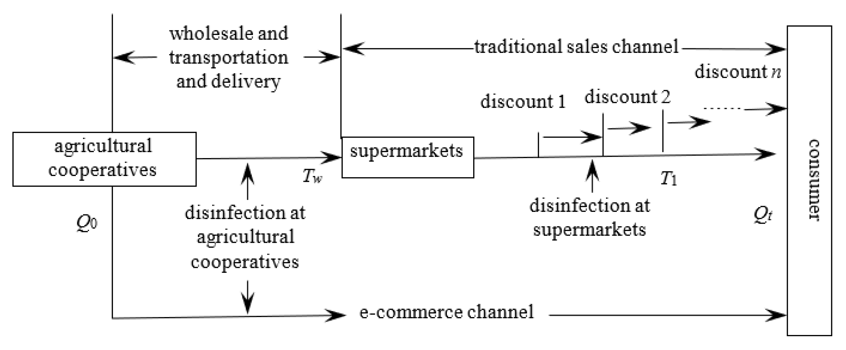
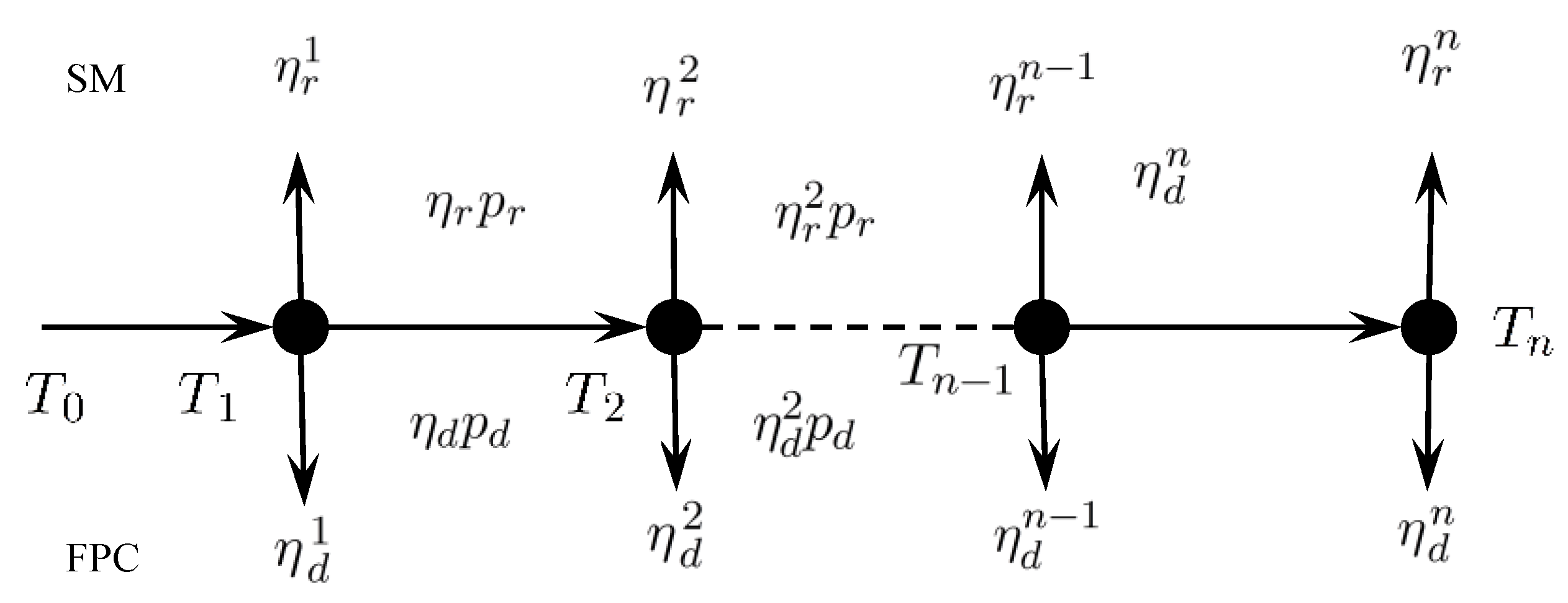
The supply chain operational system is shown in Figure 1:

The notations in this paper are shown in

Table 1. The Notations in This Paper.

c	Unit cost of fresh agricultural produce at an agricultural cooperative
g	Unit loss that occurs when products cannot be sold because of physical deterioration: i.e., the cost per unit of disposing of rotten food. Because fresh agricultural produce is worthless once it is no longer fresh, it must be disposed of. In this sense, although the scrap value of these rotten foods is zero, there are costs involved in their disposal, which means that g > c
α	Price-sensitive coefficient of a channel
β	Cross-elasticity coefficient of prices between channels. A channel’s price elasticity demand is generally higher than the cross-elasticity coefficient demand for prices between channels: i.e., α > β
TF	Quality guarantee period of fresh agricultural produce
H	Cost fixed by a particular store
U	Potential market size for fresh agricultural produce
Q	Quantity of an order supplied to a supermarket by an agriculture cooperative
$w$	Wholesale price paid by a supermarket
γ	Coefficient of fresh agricultural produce quality to demand
Dr	Market demand in the traditional sales channel
Dd	Market demand in the E-commerce channel
Pr	Supermarket price in the traditional channel
Pd	Agricultural cooperative price in the E-commerce channel
ηr	Price to discount ratio for supermarkets in the traditional channel
ηd	Price to discount ratio for agricultural cooperatives in the E-commerce channel

:

Figure 1 describes the operational process of the fresh agricultural produce supply chain. After the fresh agricultural produce is picked, agricultural cooperatives store it in a warehouse or transport it to a supermarket. At time $T_w$, the fresh products arrive at the supermarket, which then sells them to consumers. It may sell them at a discounted rate according to fresh agricultural produce characteristics or market demand. The supermarket decides when and how discounts should be applied. In the E-commerce channel, agricultural cooperatives may also apply discounts based on the same factors.

To analyze this problem, the operational process of the fresh agricultural produce supply chain should be identified (Ezzeddine et al., 2012 [24]; Kollia et al., 2021 [25]; Kurnia et al., 2016 [26]). At the first step, because quantity $Q_t$ is dependent on the behavior of agricultural cooperatives but independent of supermarkets, $Q_t$ satisfies

$$Q_t=Q_0\times \left(\frac{1}{\exp (at-b)}+\frac{1}{c+d\exp (et+f)}\right)$$

(4)

However, at the second step, quantity $Q_t$ is dependent on both agricultural cooperatives and supermarkets, so

$$\begin{array}{c}{Q}_t=Q_0\times \left[\exp \left(-a_1\left(T_w-T_0\right)+b_1\right)+\frac{1}{c_1+d_1\exp \left(e_1\left(T_w-T_0\right)+f_1\right)}\right]\\ \times \left[\exp \left(-a_2\left(t-T_w\right)-b_2\right)+\frac{1}{c_2+d_2\exp \left(e_2\left(T_0-F_{w_0}\right)+f_2\right)}\right]\end{array}$$

(5)

If the quantity of fresh agricultural produce at time $t$ is (5), it makes sense to apply a discount strategy to achieve market clearing. If a product falls below the acceptable sales quality, or if its supply far exceeds its demand, its value is 0; however, it still incurs disposal costs. If a discount strategy is applied in time, this can be avoided. In this sense, having an effective discount strategy in place is important for both agricultural cooperatives and supermarkets.

An effective discount strategy should achieve both market clearing and supply chain coordination; the latter’s primary objective is to obtain maximum profit based on the former. Second, agricultural cooperatives and supermarkets must balance their distribution with their discount strategy to ensure a reasonable profit. Third, the discount strategy should reduce the conflict between traditional and E-commerce channels to a negligible level (Tabrizi et al., 2018 [27]).

The complexity of this problem is rooted mainly in the changeable properties of the quality and quantity of fresh agricultural produce, and the conflict within their supply chain. It is therefore necessary to clarify the operational process. In the traditional channel, agricultural cooperatives transport the fresh agricultural produce to supermarkets first in the time interval $[T_0,T_w]$, where $T_0$ is the initial point in time, and $T_w$ is the point in time at which the fresh agricultural produce reaches the supermarket’s warehouse. No discount is applicable at this step because the fresh agricultural produce is not yet being sold. In the second step, $t\in [T_w,T_f]$, the fresh agricultural produce must be sold by the supermarket before it begins to rot at deadline $T_f$. The quantity and quality of fresh agricultural produce change dynamically with time, which causes the latter’s demand function to alter correspondingly, and enhances the difficulty of supply chain management. If supply and demand are equal, market clearing occurs; similarly, only if a scientific coordination mechanism is designed and implemented will the dual-channel fresh agricultural produce supply chain be coordinated. This is a necessary condition of a healthy supply chain (Gaggero et al., 2020 [12]; Xu et al., 2019 [28]; Zheng et al., 2017 [13]). To focus on the first condition of equilibrium between the supply and demand of fresh agricultural produce, the demand function must first be identified. The characteristics of this supply chain give the corresponding demand function:

$$D_r(t)=\theta U-\alpha p_r+\beta p_d+\gamma q_0{D}_1{D}_2$$

(6)

Equation (6) describes the demand for fresh agricultural produce in the traditional channel. In this process, customers buy the fresh agricultural produce from a supermarket, which causes a dynamic demand change as Equation (6). This demand function consists of four aspects: (a) the demand scale $\theta U$ of the traditional channel, driven by the demand proportion of traditional commerce $\theta$ and market scale $U$, i.e., the constant of the demand function of fresh agricultural produce; (b) sensitive demand $\alpha p_r$, driven by retail price $p_r$ and a price-sensitive coefficient in the traditional channel $\alpha$, which is accompanied by a negative linear correlation between sensitive demand and retail price; (c) cross-elasticity demand $\beta p_d$ from E-commerce trading, which is affected by demand in the E-commerce channel: if demand in E-commerce decreases in a negative linear correlation with the E-price $p_d$, demand in the traditional channel will increase, and vice versa; and (d) the demand arising from quantity loss $\gamma q_{0}f(t)$, which increases as quantity decreases. Here, the loss function has two parts: quantity loss in a certain time interval $[t_0,T_w]$, denoted by $D_1$, where $D_1=\exp \left(-a_1\left(T_w-T_0\right)+b_1\right)+\frac{1}{c_1+d_1\exp \left(e_1\left(T_w-T_0\right)+f_1\right)}$; and quantity loss from time $T_w$ to current time $t$, denoted by $D_2$, where $D_2=\exp \left(-a_2\left(t-T_w\right)-b_2\right)+\frac{1}{c_2+d_2\exp \left(e_2\left(t-T_w\right)+f_2\right)}$, which are seen in the two fractions in square brackets in Equation (6). Because these two parts are sequential processes, the demand function could be described as $D_1\times D_2$. Furthermore, if time $t\le T_w$, $D_r(t)=o(D_1)$, if $T_w<t\le T_f$, $D_r(t)=o(D_1\times D_2)$. In Equation (6), all parameters, such as $a_i,b_i,c_i,d_i,e_i,f_i,i=\{1,2\}$, are the descriptive statistical analysis results of fresh food of the cases under certain conditions.

In the E-commerce channel, agricultural cooperatives sell fresh agricultural produce directly to their customers via the internet. The sales behavior, therefore, begins at the initial point in time $t_0$, which makes them independent of supermarkets. The corresponding demand function $D_d(t)$ is:

$$\begin{array}{cc}\hfill D_d(t)& =(1-\theta )U-\alpha p_d+\beta p_r+\gamma Q_t\hfill \\ & =(1-\theta )U-\alpha p_d+\beta p_r+\gamma Q_0{D}_1\hfill \end{array}$$

(7)

Similarly, the demand function of agricultural cooperatives has four aspects in the E-commerce channel: (a) the demand scale $(1-\theta )U$ of the E-commerce channel; (b) the sensitivity demand αp_d; (c) the cross-elasticity demand βp_r in the traditional channel; and (d) demand arising from quantity loss γq₀f’(t). In the E-commerce channel, fresh agricultural produce is sold directly to customers, so the time interval is [T₀,t], which means that $f\prime (t)$ satisfies the form defined in the square brackets in Equation (7).

If the characteristics of the dual channel supply chain are reconsidered, two kinds of management must be considered: decentralized and centralized decision making (Zhai et al., 2021 [29]; Zhu et al., 2018 [30]). In the former, cooperatives and supermarkets make decisions independently, to maximize their own profits; in the latter, the two enterprises are regarded as a system, and make a decision by maximizing the profits of the system as a whole. In this case, a rational profit distribution mechanism must be designed to prevent conflict between the two sides. If both decision-making modes maximize their impact, a scientific coordination mechanism can be designed. In decentralized decision making, the supermarket’s profit can be represented as:

$$\begin{array}{cc}\hfill {\pi }_r& =p_r{\displaystyle {\int }_{T_w}^{T_f}{D}_r}(t)dt-wQ-g\left[Q-{\displaystyle {\int }_{T_w}^{T_f}{D}_r}(t)dt\right]-H\hfill \\ & =\left(p_r+g\right){\displaystyle {\int }_{T_w}^{T_f}{D}_r}(t)dt-(w+g)Q-H\hfill \\ & =\left(p_r+g\right)\left[\theta U-\alpha p_r+\beta p_d\right]\left(T_F-T_w\right)-(w+g)Q-H+\hfill \\ & \left(p_r+g\right)\gamma q_0{D}_1{D}_2\hfill \\ & \left[\frac{\ln \left[c_2\exp (-e_2(T_F-T_w)-f_2)+d_2\right]-\ln \left(c_2\exp (-f_2)+d_2\right)}{c_2{e}_2}\right]\hfill \end{array}$$

(8)

It relies on demand ${\displaystyle {\int }_{T_w}^{T_f}{D}_r(t)dt}$ in time interval $[T_w,T_f]$, the cost $wQ$, the loss arising from the quantity difference between supply and demand $g\left[Q-{\displaystyle {\int }_{T_w}^{T_f}{D}_r}(t)dt\right]$, and the disposal cost $H$ for unsaleable fresh agricultural produce. Similarly, the agricultural cooperative’s profit can be represented as:

$$\begin{array}{cc}\hfill {\pi }_d& =p_d{\displaystyle {\int }_0^{T_F}{D}_d}(t)dt+wQ-cQ-c\left({\theta }^{-1}-1\right)Q-g\left[\left({\theta }^{-1}-1\right)Q-{\displaystyle {\int }_0^{T_F}{D}_d}(t)dt\right]\hfill \\ & =Q\left(w-\frac{c+g}{\theta }+g\right)+\left(p_d+g\right)T_F\left((1-\theta )U-\alpha p_d+\beta p_r\right)\hfill \\ & +\left(p_r+g\right)\gamma q_0\times \{\frac{\left[\exp (-a_1(T_F-T_0)+b_1)-\exp b_1\right]}{a_1}\hfill \\ & +\frac{\left[\ln \left[c_1\exp (-e_1(T_F-T_0)-f_1)+d_1\right]-\ln \left(c_1\exp (-f_1)+d_1\right)\right]}{c_1{e}_1}\}\hfill \end{array}$$

(9)

The corresponding profit of the agricultural cooperative described in Equation (9) consists of the incomes from both the traditional channel $wQ$ and the E-commerce channel $p_d{\displaystyle {\int }_0^{T_F}{D}_d}(t)dt$, and the cost of the loss arising from the quantity difference between supply and demand $g\left[Q-{\displaystyle {\int }_{T_w}^{T_f}{D}_r}(t)dt\right]$, and the disposal cost of unsaleable fresh agricultural produce $H$.

To design a discount strategy that coordinates the supply chain, it is necessary to analyze the operational process and the corresponding profits of the supply chain as a whole. To do this, the supply chain should be regarded as a system that obtains the corresponding profit in the centralized decision-making mode. When the operational process is considered, the profit of supply chain ${\pi }_c$ is:

$$\begin{array}{cc}\hfill {\pi }_c& =p_r{\displaystyle {\int }_{T_w}^{T_F}{D}_r}(t)dt+p_d{\displaystyle {\int }_0^{T_F}{D}_d}(t)dt-g\left[Q-{\displaystyle {\int }_{T_w}^{T_F}{D}_r}(t)dt\right]\hfill \\ & -g\left[\left({\theta }^{-1}-1\right)Q-{\displaystyle {\int }_0^{T_F}{D}_d}(t)dt\right]-cQ-c\left({\theta }^{-1}-1\right)Q-H\hfill \\ & =\left(p_r+g\right)\left[(1-\theta )U-\alpha p_d+\beta p_r\right]\left(T_F-T_w\right)+\hfill \\ & \left(p_r+g\right)\gamma q_0\left[\exp \left(-a_1\left(T_w-T_0\right)+b_1\right)+\frac{1}{c_1+d_{1}exp\left(e_1\left(T_w-T_0\right)+f_1\right)}\right]\hfill \\ & \times \{\frac{\left[\exp (-a_2(T_F-T_w)+b_2)-\exp b_2\right]}{a_2}\hfill \\ & +\frac{\left[\ln \left[c_2\exp (-e_2(T_F-T_w)-f_2)+d_2\right]-\ln \left(c_2\exp (-f_2)+d_2\right)\right]}{c_2{e}_2}\}\hfill \\ & +\left(p_d+g\right)T_F\left((1-\theta )U-\alpha p_d+\beta p_r\right)\hfill \\ & +\left(p_d+g\right)\gamma q_0\times \{\frac{\exp (-a_1(T_F-T_0)+b_1)-\exp b_1}{a_1}\hfill \\ & +\frac{\ln \left[c_1\exp (-e_1(T_F-T_0)-f_1)+d_1\right]-\ln \left(c_1\exp (-f_1)+d_1\right)}{c_1{e}_1}\}\hfill \\ & -(c+g){\theta }^{-1}Q-H\hfill \end{array}$$

(10)

If Equations (8)–(10) are combined, the differences in profit between decentralized and centralized decision-making modes in the supply chain are calculated in Equation (11). When the sum of the supermarket and agricultural cooperative’s profits are compared with those of the fresh agricultural produce supply chain,

$$\begin{array}{cc}\hfill {\pi }_c-({\pi }_r+{\pi }_d)& =\left(p_r+g\right)(1-2\theta U)(T_F-T_w)\hfill \\ & +(\alpha -\beta )(p_r+g)(p_r-p_d)(T_F-T_w)\hfill \\ & -(p_r-p_d)\gamma q_0\times \{\frac{\exp (-a_1(T_F-T_0)+b_1)-\exp b_1}{a_1}\hfill \\ & +\frac{\ln \left[c_1\exp (-e_1(T_F-T_0)-f_1)+d_1\right]-\ln \left(c_1\exp (-f_1)+d_1\right)}{c_1{e}_1}\}\hfill \end{array}$$

(11)

Because there is no internal friction in the centralized decision-making mode, it is concluded that ${\pi }_c\ge ({\pi }_r+{\pi }_d)$. This is an essential indicator that the supply chain can be coordinated.

3. Main Results

Nonlinearity and instability mean that there are always differences between demand and supply for fresh agricultural products. Because there is a certain extent of conflict between agricultural cooperatives and supermarkets, and between traditional and E-commerce channels, it is necessary to coordinate the enterprises in the supply chain. Scientists (Gaggero et al. (2020) [12], Tang et al. (2018) [31]) have proven that discounts can redistribute profits between the enterprises in a supply chain, and consequently make it work more efficiently. When the properties of the supply chain are considered, it is concluded that the longer the discount time, the more competitive the supply. This can be expressed by an essential differential equation. If the interval of an independent variable is divided into several sub-intervals, the differential between demand and supply is small; if the sub-interval is very small, the derivative is closer to the actual function, which means that the discount times should be long enough to be influential, but not so long that they ignore the corresponding costs and effects. First, set

$$D_1=\exp \left(-a_1\left(T_n-T_{n-1}\right)+b_1\right)+\frac{1}{c_1+d_1\exp \left(e_1\left(T_n-T_{n-1}\right)+f_1\right)},$$

and $D_2=\exp \left(-a_2\left(T_w-T_0\right)+b_2\right)+\frac{1}{c_2+d_2\exp \left(e_2\left(T_w-T_0\right)+f_2\right)}$.

Additionally, set

$$\begin{gathered} {\stackrel{⌢}{D}}_i=\frac{1}{c_i+d\exp \left(e_i\left(T_n-T_{n-1}\right)+f_i\right)}-\exp \left(-a_i\left(T_n-T_{n-1}\right)+b_i\right) \\ {\tilde{D}}_i=\exp (-a_i(T_n-T_{n-1})+b_i)-\exp (-a_i(T_n-T_{n-1})+b_i), \mathrm{where} i=1,2. \end{gathered}$$

Set

$${\stackrel{⌣}{D}}_2=\ln \left[c_2\exp (-e_2(T_n-T_1)-f_2)+d_2\right]-\ln \left[c_2\exp (-e_2(T_{n-1}-T_1)-f_2)+d_2\right]$$

The corresponding conclusion of the discount strategy is given (see Theorem 1).

Theorem 1.

There exists a positive integer n and positive numbers $g_1^{n-1}(t)$ and $g_2^{n-1}(t)$ at the nth discount, where

$$\begin{array}{cc}\hfill g_1^{n-1}(t)& =\frac{\exp (-a_1(T_n-T_{n-1})+b_1)-\exp b_1}{a_1}\hfill \\ & +\frac{\ln \left[c_1\exp (-e_1(T_n-T_{n-1})-f_1)+d_1\right]-\ln \left(c_1\exp (-f_1)+d_1\right)}{c_1{e}_1}\hfill \end{array}$$

describes the profit coupled with quantity change in the E-commerce channel, and

$$\begin{array}{cc}\hfill g_2^{n-1}(t)& =\frac{\exp (-a_2(T_n-T_{n-1})+b_2)-\exp b_2}{a_2}\hfill \\ & +\frac{\ln \left[c_2\exp (-e_2(T_n-T_{n-1})-f_2)+d_2\right]-\ln \left(c_2\exp (-f_2)+d_2\right)}{c_2{e}_2}\hfill \end{array}$$

describes the profit coupled with quantity change in the traditional channel.

If the decentralized decision-making mode is adopted, the optimal discount strategies for supermarkets and agricultural cooperatives are

$${\displaystyle \sum _{n=1}^n{\left({\eta }_r^{n-1}\right)}^{*}}={\displaystyle \sum _{n=1}^n\{\frac{\theta U}{2\alpha p_r}-\frac{(1-\theta )U\alpha }{\left({\beta }^{2}2{\alpha }^2\right)p_d}+\frac{\gamma q_0}{2\alpha p_r\left(T_n-T_{n-1}\right)}{g}_2^{n-1}(t)}+\frac{\beta p_d{D}_1}{2\alpha p_r}\}$$

(12)

and

$$\begin{array}{cc}\hfill {\displaystyle \sum _{n=1}^n{\left({\eta }_d^{n-1}\right)}^{*}}& ={\displaystyle \sum _{n=1}^n\{\frac{\theta U}{2\alpha p_r}+\frac{\gamma q_0}{2\alpha p_r\left(T_n-T_{n-1}\right)}{g}_1^{n-1}(t)}+\hfill \\ & \frac{\beta }{2\alpha p_r}\frac{\gamma q_0\alpha D_2}{\left(T_n-T_{n-1}\right)\left({\beta }^2-2{\alpha }^2\right)}-\frac{(1-\theta )U\alpha }{\left({\beta }^{2}2{\alpha }^2\right)p_d}\}\hfill \end{array}$$

(13)

respectively. Under the same conditions, if the centralized decision-making mode is adopted, the optimal discount strategies for supermarkets and agricultural cooperatives are

$$\begin{array}{cc}\hfill {\displaystyle \sum _{n=1}^n{\left({\eta }_r^{n-1}\right)}^{*}}& ={\displaystyle \sum _{n=1}^n\{\frac{\gamma q_0{\stackrel{⌢}{D}}_1}{4p_r\left(T_n-T_{n-1}\right)(\beta -\alpha )}}{g}_2^{n-1}(t)-\frac{\gamma q_0{\tilde{D}}_1}{4a_1{p}_r\left(T_n-T_{n-1}\right)(\beta -\alpha )}\hfill \\ & -\frac{\gamma q_0{\tilde{D}}_1}{4p_r{a}_1\left(T_n-T_{n-1}\right)(\beta +\alpha )}+\frac{\gamma q_0\kappa \zeta }{4p_r{c}_2{e}_2\left(T_n-T_{n-1}\right)(\beta +\alpha )}\}\hfill \\ & +\frac{(2\theta -1)U}{4p_r(\beta +\alpha )}+\frac{c}{2p_r}-\frac{U}{4p_r(\beta -\alpha )}\hfill \end{array}$$

(14)

and

$$\begin{array}{cc}\hfill {\displaystyle \sum _{n=1}^n{\left({\eta }_d^{n-1}\right)}^{*}}& ={\displaystyle \sum _{n=1}^n\{\frac{\gamma q_0{\exp }^{T_w\left({\lambda }_2-{\lambda }_1\right)}{\stackrel{⌣}{D}}_2}{4p_d{c}_2{e}_2\left(T_n-T_{n-1}\right)(\beta -\alpha )}}-\frac{\gamma q_0{\tilde{D}}_1}{4p_d{a}_1\left(T_n-T_{n-1}\right)(\beta -\alpha )}\hfill \\ & +\frac{\gamma q_0{\tilde{D}}_1}{4p_d{a}_1\left(T_n-T_{n-1}\right)(\beta +\alpha )}-\frac{\gamma q_0{\stackrel{⌢}{D}}_1{\stackrel{⌣}{D}}_2}{4p_d{c}_2{e}_2\left(T_n-T_{n-1}\right)(\beta +\alpha )}\}\hfill \\ & +\frac{c}{2p_r}-\frac{U}{4p_d(\beta -\alpha )}-\frac{(2\theta -1)U}{4p_d(\beta +\alpha )}\hfill \end{array}$$

(15)

respectively.

Theorem 1 gives the optimal strategy for each stage of discount, including the optimal discount ratios for supermarkets and agricultural cooperatives using decentralized and centralized decision-making modes, respectively, if the quantity of fresh food loss satisfies Equation (4). Because transitory optimal discount ratios at discount stage n are defined by Equations (12)–(15), the supply chain can be coordinated at an arbitrary stage. There are, however, other categories of fresh food quantity loss. In certain situations, the optimal discount strategy calculated in Theorem 1 will not fit, because the properties of the quantity loss have changed. This invokes the question: Is there a more general and clearer discount strategy that coordinates the fresh agricultural produce supply chain with all possible quantity loss scenarios? Although this seems impossible, an answer is given in Theorem 2.

Theorem 2.

There exists a universal discount strategy for all scenarios of fresh agricultural produce decay. It has two categories—fixed term and drift term—which determine the optimal discount ratios. If the coordination mechanism of the decentralized decision-making mode is adopted, the fixed term of the discount ratio for supermarkets ${\displaystyle \sum _{n=1}^n{\left({\eta }_r^{n-1}\right)}^{*}}$is

$$\frac{c}{2p_r}-\frac{U}{4p_r(\beta -\alpha )}+\frac{(2\theta -1)U}{4p_r(\beta +\alpha )}$$

(16)

and the drift term is

$$\frac{\gamma q_0}{p_r}{\displaystyle \sum _{n=1}^n\left[\frac{1}{\beta -\alpha }{\displaystyle {\int }_{T_{n-1}}^{T_w}Q(t)dt}-\frac{1}{\beta +\alpha }{\displaystyle {\int }_{T_{n-1}}^{T_n}Q(t)dt}\right]}$$

(17)

The fixed term of the discount ratio for agricultural cooperatives can be generalized as

$$\frac{c}{2p_r}-\frac{U}{4p_d(\beta -\alpha )}-\frac{(2\theta -1)U}{4p_d(\beta +\alpha )}$$

(18)

and the drift term as

$$\frac{\gamma q_0}{p_d}{\displaystyle \sum _{n=1}^n\left[\frac{1}{\beta -\alpha }{\displaystyle {\int }_{T_{n-1}}^{T_w}Q(t)dt}+\frac{1}{\beta +\alpha }{\displaystyle {\int }_{T_{n-1}}^{T_n}Q(t)dt}\right]}$$

(19)

In the coordination mechanism of the centralized decision-making mode, the fixed term discounts for supermarkets and agricultural cooperatives are

$${\displaystyle \sum _{n=1}^n{\left({\eta }_r^{n-1}\right)}_{\mathrm{fixed}}^{*}}=\frac{\theta U}{2\alpha p_r}+\frac{\beta (1-\theta )U}{({\beta }^2-2{\alpha }^2)p_r}$$

(20)

and

$${\displaystyle \sum _{n=1}^n{\left({\eta }_d^{n-1}\right)}_{\mathrm{fixed}}^{*}}=\frac{(1-\theta )U\alpha }{\left({\beta }^2-2{\alpha }^2\right)p_d}$$

(21)

respectively. Similarly, the drift term discounts for supermarkets and agricultural cooperatives are

$${\displaystyle \sum _{n=1}^n{\left({\eta }_r^{n-1}\right)}_{\mathrm{drift}}^{*}}=\frac{\gamma q_0}{p_r}{\displaystyle \sum _{n=1}^n\left[\frac{1}{\alpha }{\displaystyle {\int }_{T_{n-1}}^{T_w}Q(t)dt}+\frac{\alpha }{{\beta }^2-2{\alpha }^2}{\displaystyle {\int }_{T_{n-1}}^{T_n}Q(t)dt}\right]}$$

(22)

and

$${\displaystyle \sum _{n=1}^n{\left({\eta }_d^{n-1}\right)}_{\mathrm{drift}}^{*}}=\frac{\gamma q_0}{p_d}{\displaystyle \sum _{n=1}^n\left[\frac{\alpha }{{\beta }^2-2{\alpha }^2}{\displaystyle {\int }_{T_{n-1}}^{T_w}Q(t)dt}+\frac{\alpha }{{\beta }^2-2{\alpha }^2}{\displaystyle {\int }_{T_{n-1}}^{T_n}Q(t)dt}\right]}$$

(23)

respectively.

Theorem 2 shows that whatever the quantity of fresh agricultural produce loss, there is always a universal optimal discount ratio, relying on $Q(t)$ fitting for market clearing and supply chain coordination.

4. The Single-Stage Discount Approach

In the supply chain operational process, there exists a discount point $T_1$ at which, because of conflict between demand and supply, the supply chain sells fresh agricultural produce at full price if $t<T_1$, but a discount is required if $t\ge T_1$.

If the single-stage discount strategy is used (in which the discount ratios of supermarkets and agricultural cooperatives are denoted as ${\eta }_r$ and ${\eta }_d$, respectively), the corresponding prices should be ${\eta }_d{p}_d$ and ${\eta }_r{p}_r$, respectively, after the discount. Because the discount strategy is implemented, the demand function changes accordingly. If $t<T_1$ and no discount strategy is implemented, the demand function would not change; but if $t\ge T_1$, the agricultural cooperative and supermarkets change their prices from $p_d$ and $p_r$ to ${\eta }_d{p}_d$ and ${\eta }_r{p}_r$, respectively, according to the theory of balance between supply and demand, the demand function must be changed. The properties of demand for fresh agricultural produce mean that the demand function can be regarded as a linear transformation of the original demand function. This means that in the traditional channel, if $t<T_1$,

$$\begin{array}{cc}\hfill D_{r1}(t)& =\theta U-\alpha p_r+\beta p_d+\hfill \\ & \gamma q_0\left[\exp \left(-a_1\left(T_w-T_0\right)+b_1\right)+\frac{1}{c_1+d_1\exp \left(e_1\left(T_w-T_0\right)+f_1\right)}\right]\hfill \\ & \times \left[\exp \left(-a_2\left(t-T_w\right)-b_2\right)+\frac{1}{c_2+d_2\exp \left(e_2\left(t-T_w\right)+f_2\right)}\right]\hfill \end{array}$$

(24)

The demand function consists of two parts: trend $-\alpha p_r+\beta p_d+\gamma q_{0}f(t)$ and intercept $\theta U$. The element $f(t)$ is defined in Equation (6). It is the adjustment effect for a change in market demand caused by the dynamic quantity of fresh agricultural produce in the traditional supply chain channel, and describes the decay properties of the initial quantity $q_0$ over time $t$. The agricultural cooperative’s online price $p_d$ also affects supermarket demand. Further, if $t\ge T_1$ at the discount stage,

$$\begin{array}{cc}\hfill D_{r2}(t)& =\theta U-\alpha {\eta }_r{p}_r+\beta {\eta }_d{p}_d+\hfill \\ & \gamma q_0\left[\exp \left(-a_1\left(T_w-T_0\right)+b_1\right)+\frac{1}{c_1+d_1\exp \left(e_1\left(T_w-T_0\right)+f_1\right)}\right]\hfill \\ & \times \left[\exp \left(-a_2\left(t-T_w\right)-b_2\right)+\frac{1}{c_2+d_2\exp \left(e_2\left(t-T_w\right)+f_2\right)}\right]\hfill \end{array}$$

(25)

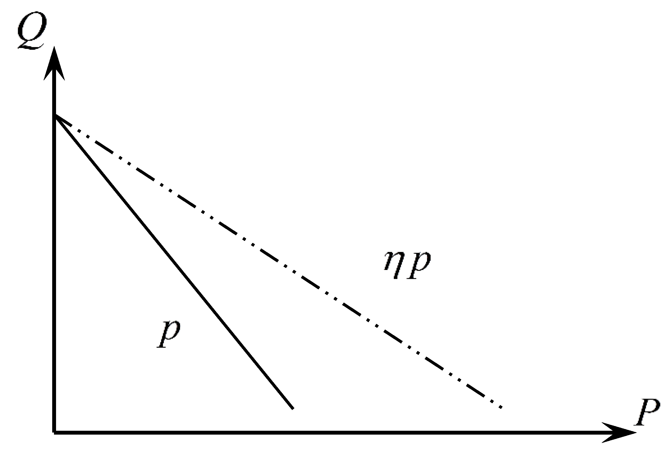
When $t\ge T_1$, the demand function shifts because the retail prices change from $p_r$ and $p_d$ to ${\eta }_r{p}_r$ and ${\eta }_d{p}_d$, respectively. If prices $p_r$ and $p_d$ form a linear scale with prices ${\eta }_r{p}_r$ and ${\eta }_d{p}_d$, respectively, then the demand function shifts accordingly, as seen in Figure 2.

Figure 2 shows the nature of the demand function’s change: i.e., there exists a discontinuous price point at which the demand function shifts from $D_{r1}$ to $D_{r2}$. The latter consists of two parts: intercept $\theta U$ and trend $-\alpha {\eta }_r{p}_r+\beta {\eta }_d{p}_d+\gamma q_{0}f(t)$.

In the E-commerce channel, transport is not necessary: customers buy fresh produce directly from agricultural cooperatives, so quantity change can only occur when the fresh agricultural produce is picked. In this case, if $t<T_1$,

$$\begin{array}{cc}\hfill D_{d1}(t)& =D_d(t)=(1-\theta )U-\alpha p_d+\beta p_r+\gamma Q_t\hfill \\ & =(1-\theta )U-\alpha p_d+\beta p_r\hfill \\ & +\gamma Q_0\times \left[\exp \left(-a_1\left(t-T_0\right)-b_1\right)+\frac{1}{c_1+d_1\exp \left(e_1\left(t-T_0\right)+f_1\right)}\right]\hfill \end{array}$$

(26)

and if $t\ge T_1$,

$$\begin{array}{cc}\hfill D_{d2}(t)& =(1-\theta )U-\alpha {\eta }_d{p}_d+\beta {\eta }_r{p}_r+\gamma Q_t\hfill \\ & =(1-\theta )U-\alpha p_d{\eta }_d+\beta p_r{\eta }_r\hfill \\ & +\gamma Q_0\times \left[\exp \left(-a_2\left(t-T_0\right)-b_2\right)+\frac{1}{c_2+d_2\exp \left(e_2\left(t-T_0\right)+f_2\right)}\right]\hfill \end{array}$$

(27)

In the traditional supply chain, the demand function is divided into two categories: Equation (26) describes the first step before the discount is applied; and Equation (27) maps the changes to supply price and demand quantity afterwards (Liu et al., 2020 [14]; Zhang et al., 2017 [32]). It is concluded that the common intercept $(1-\theta )U$ exists in both traditional and E-commerce channels, but the trend terms are different. The trend of the former channel is $-\alpha p_d+\beta p_r+\gamma q_{0}f\prime (t)$, and that of the latter is $-\alpha {\eta }_d{p}_d+\beta {\eta }_r{p}_r+\gamma q_{0}f\prime (t)$, where $f\prime (t)$ is defined in Equation (7) as the adjustment effect of the dynamic supply quantity in the E-commerce channel of the supply chain.

4.1. Price Discounts in the Decentralized Decision-Making Mode

To coordinate discounts, the profits of the supply chain and its enterprises must be analyzed. Without loss of generality, set $T_0=0$, i.e., the fresh agricultural produce is distributed immediately after it is picked, and a price discount coordination process can be specified in the decentralized decision-making mode. First, the supermarket would determine the retail price of the fresh produce based on market demand after it is delivered from the agricultural cooperative. If the retail price, discount price, market demand, purchase price and quantity of the fresh produce are fixed, the corresponding profit of the supermarket ${\pi }_r$ is

$$\begin{array}{cc}\hfill {\pi }_r& =p_r{\displaystyle {\int }_{T_w}^{T_1}{D}_{r1}(t)dt}+{\eta }_r{p}_r{\displaystyle {\int }_{T_1}^{T_F}{D}_{r2}(t)dt}-Qw-H\hfill \\ & =p_r(T_1-T_w)\left[(\theta U-\alpha p_r+\beta p_d)\right]+{\eta }_r{p}_r(T_F-T_1)\left[(\theta U-\alpha {\eta }_r{p}_r+\beta {\eta }_d{p}_d)\right]\hfill \\ & +(1+{\eta }_r)p_r\gamma q_0\times \{\frac{\exp (-a_2(T_F-T_1)+b_2)-\exp b_2}{a_2}+\hfill \\ & \frac{\ln \left[c_2\exp (-e_2(T_F-T_1)-f_2)+d_2\right]-\ln \left(c_2\exp (-f_2)+d_2\right)}{c_2{e}_2}\}-Qw-H\hfill \end{array}$$

(28)

As shown in Equation (28), the supermarket’s profit ${\pi }_r$ has two parts: one is independent of quantity change and the other is dependent on it. The former occurs in two steps (non-discount and discount), which are integral to profit density functions $\left[(\theta U-\alpha p_r+\beta p_d)\right]$ on timescale $(T_w,T_1)$ and ${\eta }_r{p}_r\left[(\theta U-\alpha {\eta }_r{p}_r+\beta {\eta }_d{p}_d)\right]$ on timescale $(T_1,T_F)$, respectively. The latter is integral to the quantity decay function in these two sequential steps, i.e., the product of dynamic prices $(1+{\eta }_r)p_r$ driven by quantity loss from both physical change and decay; and the integral quantity decay function $\frac{\exp (-a_2(T_F-T_1)+b_2)-\exp b_2}{a_2}$ of quantity change due to physical loss, and the operator $\frac{\ln \left[c_2\exp (-e_2(T_F-T_1)-f_2)+d_2\right]-\ln \left(c_2\exp (-f_2)+d_2\right)}{c_2{e}_2}$ of quantity change due to quality loss. To simplify this, the profit coupled with quantity change is denoted as $g_2(t)$, i.e.,

$$\begin{array}{cc}\hfill g_2(t)& =\frac{\exp (-a_2(T_F-T_1)+b_2)-\exp b_2}{a_2}\hfill \\ & +\frac{\ln \left[c_2\exp (-e_2(T_F-T_1)-f_2)+d_2\right]-\ln \left(c_2\exp (-f_2)+d_2\right)}{c_2{e}_2}\hfill \end{array}$$

(29)

The properties of the discount process mean that the agricultural cooperative’s profit is

$$\begin{array}{cc}\hfill {\pi }_d& =p_d{\displaystyle {\int }_{T_0}^{T_1}{D}_{d1}}(t)dt+{\eta }_d{p}_d{\displaystyle {\int }_{T_1}^{T_F}{D}_{d2}}(t)dt+Qw-Qc-\left({\theta }^{-1}-1\right)Qc\hfill \\ & =p_d(T_1-T_0)((1-\theta )U-\alpha p_d+\beta p_r)\hfill \\ & +{\eta }_d{p}_d(T_F-T_1)((1-\theta )U-\alpha p_d{\eta }_d+\beta p_r{\eta }_r)+\hfill \\ & \gamma q_0{p}_d\{\frac{\exp \left(-a_1\left(T_1-T_0\right)-b_1\right)-\exp b_1}{a_1}\hfill \\ & +\frac{\ln \left[c_1\exp (-e_1(T_1-T_0)-f_1)+d_1\right]-\ln \left(c_1\exp (-f_1)+d_1\right)}{c_1{e}_1}+\hfill \\ & {\eta }_d[\frac{\exp \left(-a_2\left(T_F-T_1\right)-b_2\right)-\exp b_2}{a_2}+\hfill \\ & \frac{\left[\ln \left[c_2\exp (-e_2(T_F-T_1)-f_2)+d_2\right]-\ln \left(c_2\exp (-f_2)+d_2\right)\right]}{c_2{e}_2}]\}\hfill \\ & +Qw-Qc-\left({\theta }^{-1}-1\right)Qc\hfill \end{array}$$

(30)

As with that of the supermarket, the profit of the agricultural cooperative consists of two sub-profits. The characteristics of the operation process mean that the wholesale process in time interval $[T_0,T_1]$ and the corresponding profit driven by quantity loss index $g_1(t)$ should be considered, and can be described in terms of quantity loss caused by physical decay $\frac{\exp \left(-a_1\left(T_1-T_0\right)-b_1\right)-\exp b_1}{a_1}$ and quality decay $\frac{\ln \left[c_1\exp (-e_1(T_1-T_0)-f_1)+d_1\right]-\ln \left(c_1\exp (-f_1)+d_1\right)}{c_1{e}_1}$, respectively. This means that

$$\begin{array}{cc}\hfill g_1(t)& =\frac{\exp \left(-a_1\left(T_1-T_0\right)-b_1\right)-\exp b_1}{a_1}\hfill \\ & +\frac{\ln \left[c_1\exp (-e_1(T_1-T_0)-f_1)+d_1\right]-\ln \left(c_1\exp (-f_1)+d_1\right)}{c_1{e}_1}\hfill \end{array}$$

(31)

The optimal discount ratios of these two enterprises are important to coordinate the supply chain; they can be decided by taking the partial derivative of ${\eta }_r$ to Equation (30).

$$\frac{\partial {\pi }_r}{\partial {\eta }_r}=\theta U{p}_r(T_F-T_1)-2\alpha {\eta }_r{p}_r^2(T_F-T_1)+\beta p_r{p}_d{\eta }_d(T_F-T_1)+p_r\gamma q_0{g}_2(t)$$

(32)

where

$$\begin{array}{cc}\hfill g_2(t)& =\frac{\exp \left(-a_2\left(t-T_1\right)-b_2\right)-\exp b_2}{a_2}\hfill \\ & +\frac{\ln \left[c_2\exp (-e_2(t-T_1)-f_2)+d_2\right]-\ln \left(c_2\exp (-f_2)+d_2\right)}{c_2{e}_2}\hfill \end{array}$$

(33)

describes the corresponding operator of the loss at the second step. If $\partial {\pi }_r/\partial {\eta }_r=0$ and $\frac{{\partial }^2{\pi }_r}{\partial {\eta }_r^2}=-2\alpha p_r^2<0$, the physical properties of this supply chain operation mean that the discount ratio of the supermarket ${\eta }_r$ satisfies

$${\eta }_r=\frac{\theta U{p}_r+\beta p_r{p}_d{\eta }_d}{2\alpha p_r^2}+\frac{p_r\gamma q_0}{2\alpha p_r^2(T_F-T_1)}\times g_2(t)$$

(34)

Similarly, the optimal discount ratio for agricultural cooperatives can be found by calculating the partial derivative of Equation (30) based on the condition of the second-order partial derivative of ${\partial }^2{\pi }_d/\partial {\eta }_d^2$. Further,

$$\begin{array}{cc}\hfill \frac{\partial {\pi }_d}{\partial {\eta }_d}& =p_d(T_F-T_1)(1-\theta )U-\left(2\alpha p_d^2-\frac{{\beta }^2{p}_d^2}{2\alpha p_r}\right){\eta }_d+\frac{\beta p_d\theta U}{2\alpha }\hfill \\ & +\frac{\beta \gamma p_r^2{p}_d{q}_0}{2\alpha p_r^2(T_F-T_1)}(g_1(t)+g_2(t))\hfill \end{array}$$

(35)

Here, $\frac{{\partial }^2{\pi }_d}{\partial {\eta }_d^2}=\frac{({\beta }^2-4{\alpha }^2)p_d^2}{2\alpha }$, and if $\beta >2\alpha$, the optimal discount ratio ${\eta }_d^{*}$ is obtained, which satisfies

$$\begin{array}{cc}\hfill {\eta }_d^{*}& =\frac{2\alpha (T_F-T_1)(1-\theta )U}{({\beta }^2-4{\alpha }^2)p_d}+\frac{\beta \theta U}{({\beta }^2-4{\alpha }^2)p_d}\hfill \\ & +\frac{\beta \gamma q_0}{({\beta }^2-4{\alpha }^2)(T_F-T_1)p_d}(g_1(t)+g_2(t))\hfill \end{array}$$

(36)

If (36) is substituted for (34),

$$\begin{array}{cc}\hfill {\eta }_r^{*}& =\frac{\theta U}{2\alpha p_r}+\frac{(T_F-T_1)(1-\theta )U\beta }{({\beta }^2-4{\alpha }^2)p_r}\hfill \\ & +\frac{\theta {\beta }^{2}U}{2\alpha p_r({\beta }^2-4{\alpha }^2)}+\frac{{\beta }^2\gamma q_0+p_r\gamma q_0({\beta }^2-4{\alpha }^2)}{2\alpha p_r({\beta }^2-4{\alpha }^2)(T_F-T_1)}{g}_2(t)\hfill \end{array}$$

(37)

Although there are differences between them, the optimal discount ratios ${\eta }_d^{*}$ and ${\eta }_r^{*}$ consist of two aspects: the trend term of the last part of Equations (36) and (37), and the constant term of the rest of these two equations. There is a decay effect in the trend term described by the integral demand function, which reflects the price and decay property coupled with dynamic quantity change. Further, the decay effects of discount ratios, which rely on the dynamic demand quantity of fresh agricultural produce, are determined by functions $g_2(t)$ and $g_1(t)+g_2(t)$, respectively. This shows that discount ratios depend on the operational process of the traditional supply chain channel. It can also be concluded that, if $\beta >2\alpha$, a minimum profit would be achieved, which is not desirable. If $\beta =2\alpha$, this is not an optimal solution; $\beta <2\alpha$ is the basic condition for the supply chain to operate normally. With this in mind, the equilibrium condition of supply and demand in supermarkets is:

$${\displaystyle {\int }_{T_0}^{T_1}{D}_{r1}}(t)dt+{\displaystyle {\int }_{T_1}^{T_F}{D}_{r2}}(t)dt=Q$$

(38)

i.e., Equation (38) can be expanded to

$$\begin{array}{c}Q=(\theta U-\alpha p_r+\beta p_d)(T_1-T_0)+(\theta U-\alpha {\eta }_r{p}_r+\beta {\eta }_d{p}_d)(T_F-T_1)\\ +\gamma q_0\left[\exp \left(-a_1\left(T_w-T_0\right)+b_1\right)+\frac{1}{c_1+d_{1}exp\left(e_1\left(T_w-T_0\right)+f_1\right)}\right]g_1(t)\\ +\gamma q_0\left[\exp \left(-a_2\left(T_F-T_1\right)+b_2\right)+\frac{1}{c_2+d_{2}exp\left(e_2\left(T_F-T_1\right)+f_2\right)}\right]g_2(t)\end{array}$$

(39)

and the constraint condition of equilibrium between supply and demand in the agricultural cooperative is

$${\displaystyle {\int }_{T_0}^{T_1}{D}_{d1}}(t)dt+{\displaystyle {\int }_{T_1}^{T_F}{D}_{d2}}(t)dt=\left({\theta }^{-1}-1\right)Q$$

(40)

Then,

$$\begin{array}{cc}\hfill \left({\theta }^{-1}-1\right)Q& =((1-\theta )U-\alpha p_d+\beta p_r)(T_1-T_0)+(1-\theta )U-\alpha p_d{\eta }_d\hfill \\ & +\beta p_r{\eta }_r(T_1-T_0)+\gamma q_0\left[g_1(t)+g_2(t)\right]\hfill \end{array}$$

(41)

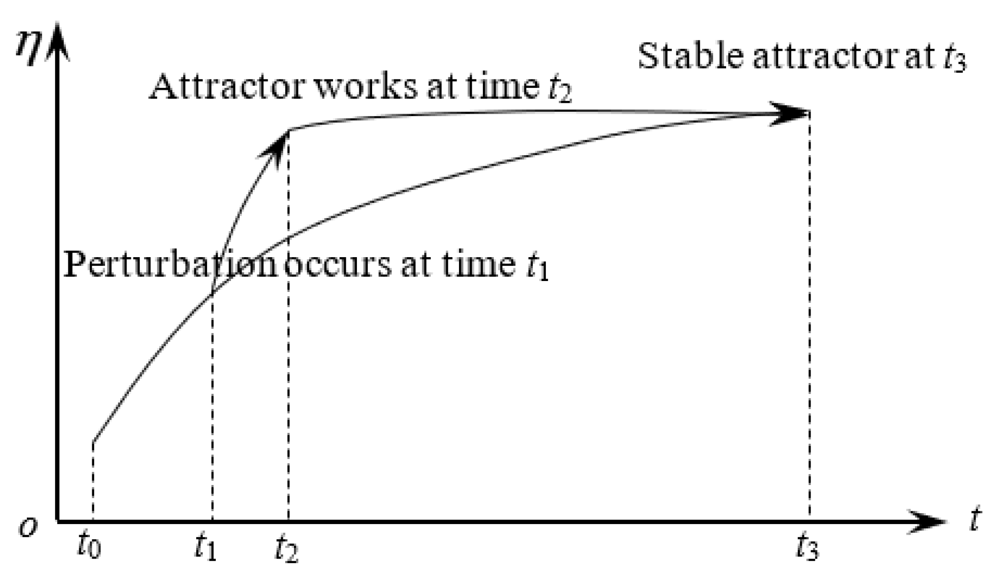
The balance of supply and demand equilibrates the dual channels of the fresh agricultural produce supply chain, and the scientific coordination mechanism defined by the discount ratios $p_r$ and $p_d$ ensures rational profit distribution based on maximizing market clearing and profit in the system as a whole. These two conditions ensure that discount ratios are always at an optimal trajectory, which stabilizes the supply chain, as shown in Figure 3.

If perturbation from the environment is added, the equilibrium between the supply and demand of fresh agricultural produce is broken, because the discount strategy can stimulate demand growth to fill it; there must be a “potential difference” attractor that pulls the deviation back to the optimal trajectory. Further, in decentralized decision making, because two enterprises make decisions independently, there are several non-synchronous behaviors that occur and entangle together in the operational process, which affects the efficiency of the supply chain.

4.2. Price Discount in the Centralized Decision-Making Mode

In centralized decision making, agricultural cooperatives and supermarkets are regarded as a whole, in which optimal prices are calculated by resolving a corresponding optimal model. Because of the relationship between market demand and system supply, and the operational properties of this supply chain, the supermarket’s retail price, the online price set by agricultural cooperatives, the supermarket’s discount ratio ${\eta }_r^{*}$, and the agricultural cooperative’s discount ratio ${\eta }_d^{*}$ must be determined. The properties of the fresh agricultural produce supply chain mean that the profit ${\pi }_c$ in the centralized decision-making mode is

$$\begin{array}{cc}\hfill {\pi }_c& =p_r{\displaystyle {\int }_{T_0}^{T_1}{D}_{r1}}(t)dt+{\eta }_r{p}_r{\displaystyle {\int }_{T_1}^{T_F}{D}_{r2}}(t)dt+p_d{\displaystyle {\int }_{T_0}^{T_1}{D}_{d1}}(t)dt\hfill \\ & +{\eta }_d{p}_d{\displaystyle {\int }_{T_1}^{T_F}{D}_{d2}}(t)dt-{\theta }^{-1}Qc-H\hfill \\ & =p_r(T_1-T_0)(\theta U-\alpha p_r+\beta p_d)+{\eta }_r{p}_r(\theta U-\alpha {\eta }_r{p}_r+\beta {\eta }_d{p}_d)(T_F-T_1)+\hfill \\ & p_d((1-\theta )U-\alpha p_d+\beta p_r)+{\eta }_d{p}_d((1-\theta )U-\alpha p_d{\eta }_d+\beta p_r{\eta }_r)-{\theta }^{-1}Qc-H\hfill \\ & +p_r\gamma q_0\left[\exp \left(-a_1\left(T_w-T_0\right)+b_1\right)+\frac{1}{c_1+d_1\exp \left(e_1\left(T_w-T_0\right)+f_1\right)}\right]g_1(t)\hfill \\ & +{\eta }_r{p}_r\gamma q_0\left[\exp \left(-a_2\left(T_F-T_1\right)+b_2\right)+\frac{1}{c_2+d_2\exp \left(e_2\left(T_F-T_1\right)+f_2\right)}\right]g_2(t)\hfill \\ & +p_d\gamma q_0{g}_1(t)+{\eta }_d{p}_d\gamma q_0{g}_2(t)\hfill \end{array}$$

(42)

Equation (42) shows that the supply chain profit has two parts: the drift term and the constant term. The constant term is $-{\theta }^{-1}Qc-H$, but the drift term is more complex. It relies on the behavior of agricultural cooperatives and supermarkets, which is determined by the price-sensitive coefficient of the channel; the price cross-elasticity coefficient of the between channels; the effective coefficient of food quality to demand; corresponding discount ratios; and the quantity loss index $g_i(t)$, where $i=1,2$. To summarize: the profit coupled with centralized decision making is defined by the constant and drift terms, which are driven by their respective prices $p_{r,d}$ and discount ratios ${\eta }_{r,d}$, coupled with the corresponding demand quantities in time intervals $[T_0,T_w)$, $[T_w,T_1)$ and $[T_1,T_F]$, respectively.

If the constraint of equilibrium conditions (38) and (40), or (39) and (41) are combined, the order quantity in the traditional channel $Q$ is

$$\begin{array}{cc}\hfill Q^{*}& =2\theta U(T_1-T_0)-\frac{\alpha \theta p_d(1+{\eta }_d)(T_1-T_0)}{1-\theta }\hfill \\ & +\frac{\beta \theta p_r(1+{\eta }_r)(T_1-T_0)}{1-\theta }+\frac{\gamma \theta q_0}{1-\theta }\left[g_1(t)+g_2(t)\right]\hfill \end{array}$$

(43)

by taking partial derivative of $Q$ from Equation (42). Substitute (43) into supply chain profit Equation (42), and $\frac{\partial {\pi }_c}{\partial {\eta }_r}=0$ and $\frac{\partial {\pi }_c}{\partial {\eta }_d}=0$, the optimal discount ratios for the agricultural cooperative and supermarket are

$$\begin{array}{cc}\hfill {\eta }_r^{*}& =\frac{\beta (1-\theta )U}{2\alpha p_d{p}_r(T_F-T_1)-{\beta }^2{p}_r{p}_d{(T_F-T_1+1)}^2}+\frac{\beta \gamma q_0(T_F-T_1+1)}{2\alpha p_r(T_F-T_1)-{\beta }^2{p}_r{(T_F-T_1+1)}^2}{g}_2(t)\hfill \\ & +\frac{\theta U(T_F-T_1)}{2\alpha p_d^2{p}_r(T_F-T_1)-{\beta }^2{p}_r{p}_d{(T_F-T_1+1)}^2{p}_d}+\hfill \\ & \frac{\alpha \gamma q_0}{2\alpha p_r(T_F-T_1)-{\beta }^2{p}_r{(T_F-T_1+1)}^2}{g}_2(t)\hfill \\ & \left[\exp \left(-a_2\left(T_F-T_1\right)+b_2\right)+\frac{1}{c_2+d_2\exp \left(e_2\left(T_F-T_1\right)+f_2\right)}\right]\hfill \end{array}$$

(44)

and

$$\begin{array}{cc}\hfill {\eta }_d^{*}& =\frac{(1-\theta )U}{\alpha p_d}+\frac{\gamma q_0}{\alpha p_d}{g}_2(t)\hfill \\ & +\frac{\beta p_r(T_F-T_1+1)}{\alpha p_d}\{\frac{\beta (1-\theta )U}{2\alpha p_r{p}_d(T_F-T_1)-{\beta }^2{p}_r{p}_d{(T_F-T_1+1)}^2}+\hfill \\ & \frac{\beta \gamma q_0(T_F-T_1+1)}{2\alpha p_r(T_F-T_1)-{\beta }^2{p}_r{(T_F-T_1+1)}^2}{g}_2(t)\hfill \\ & +\frac{\theta U(T_F-T_1)}{2\alpha p_d^2{p}_r(T_F-T_1)-{\beta }^2{p}_r{p}_d^2{(T_F-T_1+1)}^2}+\hfill \\ & \frac{\alpha p_r\gamma q_0}{2\alpha p_r(T_F-T_1)-{\beta }^2{p}_r{(T_F-T_1+1)}^2}{g}_2(t)\hfill \\ & \left[\exp \left(-a_2\left(T_F-T_1\right)+b_2\right)+\frac{1}{c_2+d_2\exp \left(e_2\left(T_F-T_1\right)+f_2\right)}\right]\}\hfill \end{array}$$

(45)

respectively. The optimal discount ratios of both ${\eta }_r^{*}$ and ${\eta }_d^{*}$ are determined by the point in time of the discount; prices $p_r$ and $p_d$; the sensitive coefficient of the price of a channel $\alpha$; the cross-elasticity coefficient of prices between channels $\beta$; and the effective coefficient of food quality to demand $g(t)$.

A comparison of the optimal discount ratios in the centralized decision-making mode described in Equations (44) and (45) with those in the decentralized decision-making mode, described in Equations (37) and (36), shows that the latter is larger than or equal to the former. This is because there are much fewer internal conflicts in centralized decision making, which makes the supply chain more effective. Further, in the centralized decision-making mode, resources, such as information, inventory and equipment, can be shared in collaborative planning, forecasting and replenishment (CPFR), which greatly improves operational efficiency [6,9]. There are, however, gaps in profit between decentralized and centralized decision-making modes, and strategies should be introduced to improve the capability of the latter.

5. Optimizing the Multi-Stage Discount Strategy

5.1. Market Clearing in Multi-Stage Discounts

The quality of fresh agricultural produce deteriorates over time, which means that several stages of discount are necessary. This is because as the quantity and quality of fresh agricultural produce decline, the price elasticity coefficient becomes smaller, and the demand function correspondingly becomes concave. The graph of the demand function is described approximately in Figure 4.

Figure 4 shows the properties of the demand function and the way the effects of discounts vary at different times. As discount times increase, supply matches demand more closely.

Multi-stage discounts follow a process: Once the quality or quantity reaches a certain low threshold, the corresponding price discount ratio ${\eta }_{r,d}^k$ must be introduced to compensate for the loss that occurs because of the mismatch between supply and demand, and to redistribute profit rationally between supermarkets and agricultural cooperatives. Here, $k$ is the $k^{th}$ discount stage, and $r$ and $d$ represent the supermarket and cooperative, respectively. In the operational properties of the fresh agricultural produce supply chain, discount behaviors always occur after time $T_w$, after which the multi-stage discount process can be analyzed. First, if the first discount time $T_1>T_w$, the corresponding process is as described in Figure 5.

Because the price in one discount stage must differ from that in another, the corresponding demand function of the dual-channel supply chain relies on the order $j\in \{1,2,\dots ,n\}$ of the discount stage. According to the properties of the multi-stage discount strategy in the supply chain, the price in time interval $(T_i,T_{i+1}]$ should be ${\eta }_r^{n-1}{p}_r$ or ${\eta }_d^{n-1}{p}_d$ before the discount stage $n$; so, the corresponding demand function at the $n^{\mathrm{th}}$ stage is determined by the discount ratio ${\eta }_r^{n-1}$ at the previous stage. Generally, ${\eta }_r^n$ is smaller than ${\eta }_r^{n-1}$ to ensure both market clearing and fair profit distribution. According to the properties of multi-stage discounts in the fresh agricultural produce supply chain, the demand function of the supermarket in the discount stage $n$ is:

$$\begin{array}{cc}\hfill D_{rn}(t)& =\theta U-\alpha {\eta }_r^{n-1}{p}_r+\beta {\eta }_d^{n-1}{p}_d\hfill \\ & +\gamma q_0\left[\exp \left(-a_1\left(T_w-T_0\right)+b_1\right)+\frac{1}{c_1+d_1\exp \left(e_1\left(T_w-T_0\right)+f_1\right)}\right]\hfill \\ & \times \left[\exp \left(-a_2\left(t-T_w\right)-b_2\right)+\frac{1}{c_2+d_2\exp \left(e_2\left(t-T_w\right)+f_2\right)}\right]\hfill \end{array}$$

(46)

Similarly, the demand function of the E-commerce channel in the discount stage $n$ of the agricultural cooperative is:

$$\begin{array}{cc}\hfill D_{dn}(t)& =(1-\theta )U-\alpha {\eta }_d^{n-1}{p}_d+\beta {\eta }_r^{n-1}{p}_r\hfill \\ & +\gamma q_0\times \left[\exp \left(-a_1\left(t-T_0\right)-b_1\right)+\frac{1}{c_1+d_1\exp \left(e_1\left(t-T_0\right)+f_1\right)}\right]\hfill \end{array}$$

(47)

Equations (46) and (47) show that within each time interval $(T_{n-1},T_n)$ of the discount, the demand is deterministic due to the deterministic price. When the new discount ratio ${\eta }_n$ is introduced at time $T_n$, however, the demand shifts from what is decided by discount ratio η_{n − 1} to the ratio decided by η_n, according to Equation (46) or (47). This means that demand is a piecewise function, and the points at time $T_i,i=1,2,\dots$ are all discontinuity points of the second kind. As previously analyzed, the discount ratio is an attenuation function with multiple discount times $i,i=1,2,\dots$, to which the demand function adjusts correspondingly.

Further, because of the anchoring effect, the discount works quickly if and only if its stages occur over a short period. In this case, the state at the next stage is dependent on that of the one that precedes it. To study the multi-stage discount strategy in supply chain coordination, this property must be thoroughly understood. The demand in different stages of this discount process can be regarded as a martingale process (Jin-you strategy (Hu et al., 2019 [33]), where

$$P(D_{r,n}(t)|D_{r,n-1},D_{r,n-2},\dots ,D_{r,1})=P(D_{r,n-1})$$

(48)

with $n,n=1,2,\dots$, i.e., $E[P(D_{r,n}(t)-D_{r,n-1}|D_{r,n-1},D_{r,n-2},\dots ,D_{r,1})]=0$. Each discount stage can then be analyzed independently, and based on this, the multi-stage discount strategy can be understood as a whole.

As previously explained, there are always two kinds of decision making in the supply chain coordination process that can be selected. Decentralized decision making is similar to the single-stage discount process to a certain extent. At some stage, however, the demand function is different because the price changes, so the total profit is the sum of the profits at each stage of discount. In this case, the supermarket’s profit becomes:

$$\begin{array}{l}{\pi }_r={\displaystyle \sum _{n=1}^n{\eta }_r^{n-1}}{p}_r{\displaystyle {\int }_{T_{n-1}}^{T_n}{D}_{rn}}(t)dt-Qw-H\\ ={\displaystyle \sum _{n=1}^n\{{\eta }_r^{n-1}{p}_r(\theta U-\alpha {\eta }_r^{n-1}{p}_r+\beta {\eta }_d^{n-1}{p}_d)(T_n-T_{n-1})+}\\ {\eta }_r^{n-1}{p}_r\gamma q_0\left[\exp \left(-a_1\left(T_w-T_0\right)+b_1\right)+\frac{1}{c_1+d_1\exp \left(e_1\left(T_w-T_0\right)+f_1\right)}\right]g_2^{n-1}(t)-Qw-H\end{array}$$

(49)

Equations (28) and (49) differ slightly, because each discount stage is independent of discount time but dependent on demand, and demand satisfies the property of the martingale strategy in Equation (48). If the discount ${\eta }_i$ is a constant, the ratio at the $n\mathrm{th}$ discount becomes ${\eta }_i^n,n=1,2,\dots$, and the profit at each stage can be calculated by Equation (49). According to a similar process and method and considering its dynamic nature, the agricultural cooperative’s profit would be:

$$\begin{array}{cc}\hfill {\pi }_d& ={\displaystyle \sum _{n=1}^n{\eta }_d^{n-1}}{p}_d{\displaystyle {\int }_{T_{n-1}}^{T_n}{D}_{dn}}(t)dt+Qw-Qc-\left({\theta }^{-1}-1\right)Qc\hfill \\ & ={\displaystyle \sum _{n=1}^n{\eta }_d^{n-1}{p}_d\{\left[(1-\theta )U-\alpha {\eta }_d^{n-1}{p}_d+\beta {\eta }_r^{n-1}{p}_r\right](T_n-T_{n-1})}\hfill \\ & +\gamma q_0\times (g_1^{n-1}(t)+g_2^{n-1}(t))\}+Qw-Qc-\left({\theta }^{-1}-1\right)Qc\hfill \end{array}$$

(50)

As discussed, the corresponding constraint conditions for equilibrium between supply and demand in the traditional channel must be addressed. In dynamic coordination terms, the supply chain is coordinated as a whole if it is coordinated at each stage using certain strategies. Regardless of coordinative strategies, however, market clearing is crucial to the supply chain to obtain maximum profit, which requires that

$${\displaystyle \sum _{n=1}^n{\displaystyle {\int }_{T_{n-1}}^{T_n}{D}_{rn}}}(t)dt=Q$$

i.e., if and only if the supply of fresh agricultural produce matches demand, there is no internal conflict in the supply chain. If demand $D_n(t)$ is expanded at the nth discount stage, then

$$\begin{array}{cc}\hfill Q& ={\displaystyle \sum _{n=1}^n\{\left(\theta U-\alpha {\eta }_r^{n-1}{p}_r+\beta {\eta }_d^{n-1}{p}_d\right)(T_n-T_{n-1})+}\hfill \\ & +\gamma q_0\left[\exp \left(-a_1\left(T_w-T_0\right)+b_1\right)+\frac{1}{c_1+d_1\exp \left(e_1\left(T_w-T_0\right)+f_1\right)}\right]g_2^{n-1}(t)\}\hfill \end{array}$$

(51)

where

$$\begin{array}{cc}\hfill g_2^{n-1}(t)& =\frac{\exp (-a_2(T_n-T_{n-1})+b_2)-\exp b_2}{a_2}\hfill \\ & +\frac{\ln \left[c_2\exp (-e_2(T_n-T_{n-1})-f_2)+d_2\right]-\ln \left(c_2\exp (-f_2)+d_2\right)}{c_2{e}_2}\hfill \end{array}$$

describes the profit coupled with the quantity change in the traditional channel, and

$$\begin{array}{c}{g}_1^{n-1}(t)=\frac{\exp (-a_1(T_n-T_{n-1})+b_1)-\exp b_1}{a_1}\\ +\frac{\ln \left[c_1\exp (-e_1(T_n-T_{n-1})-f_1)+d_1\right]-\ln \left(c_1\exp (-f_1)+d_1\right)}{c_1{e}_1}\end{array}$$

describes the profit coupled with the quantity change in the E-commerce channel.

According to the same method, the corresponding constraint conditions for equilibrium between supply and demand in the E-commerce supply chain channel are

$${\displaystyle \sum _{n=1}^n{\displaystyle {\int }_{T_{n-1}}^{T_n}{D}_{dn}}}(t)dt=\left({\theta }^{-1}-1\right)Q$$

i.e.,

$$\left({\theta }^{-1}-1\right)Q={\displaystyle \sum _{n=1}^n\{\left[(1-\theta )U-\alpha {\eta }_d^{n-1}{p}_d+\beta {\eta }_r^{n-1}{p}_r\right](T_n-T_{n-1})+\gamma q_0{g}_1^{n-1}(t)]\}}$$

(52)

Equations (51) and (52) show that the equilibrium between supply and demand is important to the sale of fresh agricultural produce. Because the produce must be fresh, the demand functions vary at different stages, and this equilibrium is broken. It is not necessary for supply to be equal to demand at every stage, but the total demand must be equal to the total supply in all stages as a whole. This means that the respective conditions under both decentralized and centralized decision-making modes are much complex. The equilibrium in the operational process as a whole can be understood as a degenerate distribution in the equilibrium at each stage of discount. Although this degeneration is not strictly correct (because the local equilibrium in sequential small timescales in accordance with discount stages is a sufficient but not essential condition), it is a reasonable alternative method.

The coordination of the supply chain with multi-stage discounts is analyzed in Section 5.2.

5.2. Optimal Discount Ratios in Multi-Stage Discount Strategies

In the decentralized decision-making mode, like in the single-stage discount process, the supermarket sets the retail price based on market demand. A reasonable discount ratio ${\eta }_r^{n-1}$ can be set to encourage demand, which in turn changes the demand quantity. This means the agricultural cooperative must produce the new discount ratio ${\eta }_d^{n-1}$. In this aspect, there is no difference between single- and multi-stage discount strategies.

Combine Equations (49)–(52), then take partial derivative for ${\eta }_r^{n-1}$ and ${\eta }_d^{n-1}$ from (49) and (50), respectively; the partial derivative $\partial {\pi }_r/\partial {\eta }_r^{n-1}$ of the nth discount stage is:

$$\begin{array}{cc}\hfill \frac{\partial {\pi }_r}{\partial {\eta }_r^{n-1}}& ={\displaystyle \sum _{n=1}^n\{\left(T_n-T_{n-1}\right)\left[\theta U{p}_r-2\alpha {\eta }_r^{n-1}{p}_r^2+\beta p_r{p}_d{\eta }_d^{n-1}\right]}\hfill \\ & +\gamma q_0{p}_r\left[\exp \left(-a_1\left(T_w-T_0\right)+b_1\right)+\frac{1}{c_1+d_1\exp \left(e_1\left(T_w-T_0\right)+f_1\right)}\right]g_2^{n-1}(t)\}\hfill \end{array}$$

(53)

Equation (53) shows that $\frac{{\partial }^2{\pi }_r}{\partial {\left({\eta }_r^{n-1}\right)}^2}<0$. These multiple stages of the discount process are not independent of each other, but rather work as a system. The optimal sequential discount ratios must be determined systematically. If the properties of the discount strategy and Equation (53) are considered, the function of the discount ratio of the retail price of fresh agricultural produce in the traditional channel is:

$$\begin{array}{cc}\hfill {\displaystyle \sum _{n=1}^n{\eta }_r^{n-1}}& ={\displaystyle \sum _{n=1}^n\left[\frac{\theta U}{2\alpha p_r}+\frac{\beta p_d{\eta }_d^{n-1}}{2\alpha p_r}\right]}\hfill \\ & +{\displaystyle \sum _{n=1}^n\{\frac{\gamma q_0}{2\alpha p_r\left(T_n-T_{n-1}\right)}\left[\exp \left(-a_1\left(T_w-T_0\right)+b_1\right)+\frac{1}{c_1+d_1\exp \left(e_1\left(T_w-T_0\right)+f_1\right)}\right]}\hfill \\ & g_2^{n-1}(t)\}\hfill \end{array}$$

(54)

Equation (54) shows that the discount ratio ${\eta }_r^{n-1}$ of the supermarket’s retail price relies on the discount ratio ${\eta }_d^{n-1}$ of the agricultural cooperative, and the mapping between them is relatively complex. If the solution to Equation (54) is ${\eta }_r^{*}={\eta }_r\left({\eta }_d\right)$, replace it into the profit function of the cooperative; then, taking the first order partial derivative to ${\eta }_d^{n-1}$, we have

$$\frac{\partial {\pi }_d}{\partial {\eta }_d^{n-1}}={\displaystyle \sum _{n=1}^n\{\left(T_n-T_{n-1}\right)\left[(1-\theta )U{p}_d-2\alpha {\eta }_d^{n-1}{p}_d^2+\frac{{\beta }^2{p}_d^2{\eta }_d^{n-1}}{\alpha }\right]+\gamma q_0{p}_d{g}_1^{n-1}(t)\}}$$

(55)

It can also be seen that $\alpha >\beta$ and $\frac{{\partial }^2{\pi }_d}{\partial {\left({\eta }_d^{n-1}\right)}^2}={\displaystyle \sum _{n=1}^n\frac{\left(T_n-T_{n-1}\right)\left({\beta }^2-2{\alpha }^2\right)p_d^2}{\alpha }}<0$. According to the analysis method used in ${\eta }_r^{n-1}$, the optimal price discount ratio ${\eta }_d^n$ of a fresh agricultural produce from an agricultural cooperative in the E-commerce channel is:

$$\begin{array}{cc}\hfill {\displaystyle \sum _{n=1}^n{\left({\eta }_d^{n-1}\right)}^{*}}& ={\displaystyle \sum _{n=1}^n\{\frac{\theta U}{2\alpha p_r}+\frac{\gamma q_0}{2\alpha p_r\left(T_n-T_{n-1}\right)}{g}_1^{n-1}(t)}+\hfill \\ & \frac{\beta }{2\alpha p_r}\frac{\gamma q_0\alpha }{\left(T_n-T_{n-1}\right)\left({\beta }^2-2{\alpha }^2\right)}[\exp \left(-a_2\left(T_w-T_0\right)+b_2\right)\hfill \\ & +\frac{1}{c_2+d_2\exp \left(e_2\left(T_w-T_0\right)+f_2\right)}]-\frac{(1-\theta )U\alpha }{\left({\beta }^{2}2{\alpha }^2\right)p_d}\}\hfill \end{array}$$

(56)

Similarly, if ${\eta }_d^{*}$. is inserted into the reverse function of response function ${\eta }_r^{*}={\eta }_r\left({\eta }_d\right)$, the optimal discount ratio ${\eta }_r^{*}$ in the traditional channel is:

$$\begin{array}{cc}\hfill {\displaystyle \sum _{n=1}^n{\left({\eta }_r^{n-1}\right)}^{*}}& ={\displaystyle \sum _{n=1}^n\{\frac{\theta U}{2\alpha p_r}-\frac{(1-\theta )U\alpha }{\left({\beta }^{2}2{\alpha }^2\right)p_d}+\frac{\gamma q_0}{2\alpha p_r\left(T_n-T_{n-1}\right)}{g}_2^{n-1}(t)}\hfill \\ & +\frac{\beta p_d}{2\alpha p_r}\left[\exp \left(-a_1\left(T_n-T_{n-1}\right)+b_1\right)+\frac{1}{c_1+d_1\exp \left(e_1\left(T_n-T_{n-1}\right)+f_1\right)}\right]\}\hfill \end{array}$$

(57)

In the decentralized decision-making mode in this dual channel supply chain, agricultural cooperatives and supermarkets work independently to pursue their own optimal profits. Because of this, the analytical solution for the optimal price discount ratio ${\eta }_d$ of the agricultural cooperative, and the discount ratio ${\eta }_r$ of the supermarket maximize both market clearing and the profits of each party. An analytical process that combines Equations (56) and (57) should therefore be applied to ascertain the optimal profits for agricultural cooperatives and supermarkets, respectively:

$${\pi }_r^{*}={\displaystyle \sum _{n=1}^n{\left({\eta }_r^{n-1}\right)}^{*}}{p}_r{\displaystyle {\int }_{T_{n-1}}^{T_n}{D}_{rn}}(t)dt-Qw-H$$

(58)

$${\pi }_d^{*}={\displaystyle \sum _{n=1}^n{\left({\eta }_d^{n-1}\right)}^{*}}{p}_d{\displaystyle {\int }_{T_{n-1}}^{T_n}{D}_{dn}}(t)dt+Qw-Qc-\left({\theta }^{-1}-1\right)Qc$$

(59)

Similarly, the profit of the supply chain as a whole would then be:

$$\begin{array}{cc}\hfill {\pi }_c& ={\displaystyle \sum _{n=1}^n{\eta }_r^{n-1}}{p}_r{\displaystyle {\int }_{T_{n-1}}^{T_n}{D}_{rn}}(t)dt+{\displaystyle \sum _{n=1}^n{\eta }_d^{n-1}}{p}_d{\displaystyle {\int }_{T_{n-1}}^{T_n}{D}_{dn}}(t)dt-Qc-\left({\theta }^{-1}-1\right)Qc-H\hfill \\ & ={\displaystyle \sum _{n=1}^n\{{\eta }_r^{n-1}{p}_r(\theta U-\alpha {\eta }_r^{n-1}{p}_r+\beta {\eta }_d^{n-1}{p}_d)(T_n-T_{n-1})+}\hfill \\ & {\eta }_r^{n-1}{p}_r\gamma q_0\left[\exp \left(-a_1\left(T_w-T_0\right)+b_1\right)+\frac{1}{c_1+d_1\exp \left(e_1\left(T_w-T_0\right)+f_1\right)}\right]g_2^{n-1}(t)\hfill \\ & +{\displaystyle \sum _{n=1}^n{\eta }_d^{n-1}{p}_d\{\left[(1-\theta )U-\alpha {\eta }_d^{n-1}{p}_d+\beta {\eta }_r^{n-1}{p}_r\right](T_n-T_{n-1})+\gamma q_0{g}_1^{n-1}(t)\}}\hfill \\ & -Qc-\left({\theta }^{-1}-1\right)Qc-H\hfill \end{array}$$

(60)

Taking the first and second partial derivatives of ${\eta }_{r,d}^{n-1}$ for Equation (60), the second Hesse matrix $S$ of ${\pi }_c$ to ${\eta }_r^{n-1}$ and ${\eta }_d^{n-1}$ would be:

$$S=\left[\begin{array}{cc}\frac{{\partial }^2{\pi }_c}{\partial {\left({\eta }_r^{n-1}\right)}^2}& \frac{{\partial }^2{\pi }_c}{\partial {\eta }_r^{n-1}{\eta }_d^{n-1}}\\ \frac{{\partial }^2{\pi }_c}{\partial {\eta }_d^{n-1}{\eta }_r^{n-1}}& \frac{{\partial }^2{\pi }_c}{\partial {\left({\eta }_d^{n-1}\right)}^2}\end{array}\right]=\left[\begin{array}{cc}-2\alpha p_r{}^2{\displaystyle \sum _{n=1}^n\left(T_n-T_{n-1}\right)}& 2\beta p_r{p}_d{\displaystyle \sum _{n=1}^n\left(T_n-T_{n-1}\right)}\\ 2\beta p_r{p}_d{\displaystyle \sum _{n=1}^n\left(T_n-T_{n-1}\right)}& -2\alpha p_d^2{\displaystyle \sum _{n=1}^n\left(T_n-T_{n-1}\right)}\end{array}\right]$$

(61)

where $|S|=4\left({\alpha }^2-{\beta }^2\right)p_r^2{p}_d^2{\left({\displaystyle \sum _{n=1}^n\left(T_n-T_{n-1}\right)}\right)}^2,\alpha >\beta ,T_n>T_{n-1}$, and $\left|S\right|>0$. Because $-2\alpha p_r^2{\displaystyle \sum _{n=1}^n\left(T_n-T_{n-1}\right)}<0$ in matrix S, the second Hesse matrix of ${\pi }_c$ to ${\eta }_r^{n-1}$ and ${\eta }_d^{n-1}$ is a negative definite matrix, which means that ${\pi }_c$ is a joint concave function of ${\eta }_r^{n-1}$ and ${\eta }_d^{n-1}$. The quantity of fresh agricultural produce in the supply chain is therefore:

$$\begin{array}{cc}\hfill Q& ={\displaystyle \sum _{n=1}^n\theta }\left(T_n-T_{n-1}\right)\left[U+(\beta -\alpha )\left({\eta }_d^{n-1}{p}_d+{\eta }_r^{n-1}{p}_r\right)\right]+{\displaystyle \sum _{n=1}^n\frac{\theta \gamma q_0}{2\alpha p_r\left(T_n-T_{n-1}\right)}{g}_2^{n-1}(t)}\hfill \\ & +{\displaystyle \sum _{n=1}^n\theta \gamma q_0\left[\exp \left(-a_1\left(T_w-T_0\right)+b_1\right)+\frac{1}{c_1+d_1\exp \left(e_1\left(T_w-T_0\right)+f_1\right)}\right]}\hfill \end{array}$$

(62)

In the centralized decision-making mode, although the steps of the multi-stage discount are relatively complex, the basic principle is the same as in the single-stage discount process. If the optimal quantity of fresh agricultural produce is inserted into the supply chain profit function in the centralized decision-making mode, the derivative can be ascertained based on discount ratios ${\eta }_r^{n-1}$ and ${\eta }_d^{n-1}$. For the profit function of agricultural cooperatives and supermarkets in the centralized decision-making mode, the optimal discount ratios ${({\eta }_r^{n-1})}^{*}$ and ${({\eta }_d^{n-1})}^{*}$ are

$$\begin{array}{cc}\hfill {\displaystyle \sum _{n=1}^n{\left({\eta }_r^{n-1}\right)}^{*}}& ={\displaystyle \sum _{n=1}^n\{\frac{\gamma q_0}{4p_r\left(T_n-T_{n-1}\right)(\beta -\alpha )}}{g}_2^{n-1}(t)\times \hfill \\ & \left[\frac{1}{c_1+d\exp \left(e_1\left(T_n-T_{n-1}\right)+f_1\right)}-\exp \left(-a_1\left(T_n-T_{n-1}\right)+b_1\right)\right]\hfill \\ & -\frac{\gamma q_0\left(\exp (-a_1(T_n-T_{n-1})+b_1)-\exp (-a_1(T_n-T_{n-1})+b_1)\right)}{4a_1{p}_r\left(T_n-T_{n-1}\right)(\beta -\alpha )}\hfill \\ & -\frac{\gamma q_0\left(\exp (-a_1(T_n-T_{n-1})+b_1)-\exp (-a_1(T_n-T_{n-1})+b_1)\right)}{4p_r{a}_1\left(T_n-T_{n-1}\right)(\beta +\alpha )}\hfill \\ & +\frac{\gamma q_0}{4p_r{c}_2{e}_2\left(T_n-T_{n-1}\right)(\beta +\alpha )}\hfill \\ & \left[\frac{1}{c_1+d\exp \left(e_1\left(T_w-T_1\right)+f_1\right)}-\exp \left(-a_1\left(T_w-T_1\right)+b_1\right)\right]\times \hfill \\ & [\ln \left[c_2\exp (-e_2(T_n-T_1)-f_2)+d_2\right]\hfill \\ & -\ln \left[c_2\exp (-e_2(T_{n-1}-T_1)-f_2)+d_2\right]]\}+\frac{(2\theta -1)U}{4p_r(\beta +\alpha )}+\frac{c}{2p_r}-\frac{U}{4p_r(\beta -\alpha )}\hfill \end{array}$$

(63)

and

$$\begin{array}{cc}\hfill {\displaystyle \sum _{n=1}^n{\left({\eta }_d^{n-1}\right)}^{*}}& ={\displaystyle \sum _{n=1}^n\{\frac{\gamma q_0{\exp }^{T_w\left({\lambda }_2-{\lambda }_1\right)}}{4p_d{c}_2{e}_2\left(T_n-T_{n-1}\right)(\beta -\alpha )}[\ln \left[c_2\exp (-e_2(T_n-T_1)-f_2)+d_2\right]}\hfill \\ & -\ln \left[c_2\exp (-e_2(T_{n-1}-T_1)-f_2)+d_2\right]]\hfill \\ & -\frac{\gamma q_0\left(\exp (-a_1(T_n-T_{n-1})+b_1)-\exp (-a_1(T_n-T_{n-1})+b_1)\right)}{4p_d{a}_1\left(T_n-T_{n-1}\right)(\beta -\alpha )}\hfill \\ & +\frac{\gamma q_0\left(\exp (-a_1(T_n-T_{n-1})+b_1)-\exp (-a_1(T_n-T_{n-1})+b_1)\right)}{4p_d{a}_1\left(T_n-T_{n-1}\right)(\beta +\alpha )}\hfill \\ & -\frac{\gamma q_0}{4p_d{c}_2{e}_2\left(T_n-T_{n-1}\right)(\beta +\alpha )}\times [\ln \left[c_2\exp (-e_2(T_n-T_1)-f_2)+d_2\right]\hfill \\ & -\ln \left[c_2\exp (-e_2(T_{n-1}-T_1)-f_2)+d_2\right]]\times \hfill \\ & \left[\frac{1}{c_1+d\exp \left(e_1\left(T_n-T_{n-1}\right)+f_1\right)}-\exp \left(-a_1\left(T_n-T_{n-1}\right)+b_1\right)\right]\}\hfill \\ & +\frac{c}{2p_r}-\frac{U}{4p_d(\beta -\alpha )}-\frac{(2\theta -1)U}{4p_d(\beta +\alpha )}\hfill \end{array}$$

(64)

respectively, where $\frac{\partial {\pi }_c}{\partial {\eta }_r^{n-1}}=0,\frac{\partial {\pi }_c}{\partial {\eta }_d^{n-1}}=0$. Further, the optimal profit of the supply chain ${\pi }_c^{*}$ in the centralized decision-making mode is:

$${\pi }_c^{*}={\displaystyle \sum _{n=1}^n{\left({\eta }_r^{n-1}\right)}^{*}}{p}_r{\displaystyle {\int }_{T_{n-1}}^{T_n}{D}_{rn}}(t)dt+{\displaystyle \sum _{n=1}^n{\left({\eta }_d^{n-1}\right)}^{*}}{p}_d{\displaystyle {\int }_{T_{n-1}}^{T_n}{D}_{dn}}(t)dt-Qc-\left({\theta }^{-1}-1\right)Qc-H$$

(65)

It has been proven that the profit produced in centralized decision making is greater than or equal to that of decentralized decision making. Accordingly, the corresponding discount ratios are also more reliable (Tran 2018 [34]).

Although centralized decision making is better at coordinating the supply chain and ensuring market clearance, the synchronization between supermarket and agricultural cooperative must be strictly controlled. As a result, decentralized decision making is often introduced (Neubert et al., 2018 [35]; Singh et al., 2015 [36]; Stranieri et al., 2018 [37]).

6. Discussion and Conclusions

6.1. Other Scenarios and Comparisons

Although there are several kinds of quantity loss, this paper examines the case of dual decay with quality and quantity loss. This hypothesis, however, is not strictly correct, because other scenarios can occur under certain conditions (Belkhatir et al., 2020 [38]; Suhail et al., 2020 [39]). For example, what strategy should be used if the quantity loss is not what Equation (3) defines, or if a demand disruption occurs, or if a series of substitutes for fresh agricultural products are considered synchronously? What we cared is not just the coordination strategy in the particular case defined in this paper, but a universal coordination strategy for all possible cases. All scenarios can be described by several specific parameters, and if they are taken as fixed constants, the scenario becomes deterministic (Inoue et al., 2020 [40]; Tominac et al., 2020 [41]). To draw a universal conclusion for discount coordination, other scenarios should be discussed. Because this is too complex to analyze in the scope of this paper, we examined a coordination strategy for the different kinds of quantity loss of fresh agricultural produce. A simple case of quantity loss that satisfies exponential distribution $\exp (-\lambda (t-t_0))$ is discussed in the following paragraph.

6.1.1. The Discount Strategy for Quantity Loss That Satisfies Exponential Distribution $\exp (-\lambda (t-t_0))$

This is a degenerate distribution of the model constructed in this paper that ignores quantity loss $Q_0{\left(c+d\exp (et+f)\right)}^{-1}$ arising from decay. Using the same analysis method and process, the optimal discount ratio of the agricultural cooperative in a single-stage discount strategy is considered. The optimal discount ratios of ${\eta }_d^{*}$ and ${\eta }_r^{*}$ in the decentralized decision-making mode would then be

$${\eta }_d^{*}=\frac{\gamma q_0\left({\mathrm{e}}^{-{\lambda }_1{T}_F}-{\mathrm{e}}^{-{\lambda }_1{T}_1}\right)}{{\lambda }_1\left(T_F-T_1\right)p_d\left({\beta }^2-2{\alpha }^2\right)}+\frac{\alpha (1-\theta )U}{2{\alpha }^2{p}_d-{\beta }^2{p}_d}$$

(66)

and

$$\begin{array}{cc}\hfill {\eta }_r^{*}& =\frac{\theta U}{2\alpha p_r}+\frac{\gamma q_0{\mathrm{e}}^{T_w\left({\lambda }_2-{\lambda }_1\right)}\left({\mathrm{e}}^{-{\lambda }_2{T}_1}-{\mathrm{e}}^{-{\lambda }_2{T}_F}\right)}{2\alpha p_r{\lambda }_2\left(T_F-T_1\right)}\hfill \\ & +\frac{\beta p_d}{2\alpha p_r}\left[\frac{\gamma q_0\left({\mathrm{e}}^{-{\lambda }_1{T}_F}-{\mathrm{e}}^{-{\lambda }_1{T}_1}\right)}{{\lambda }_1\left(T_F-T_1\right)p_d\left({\beta }^2-2{\alpha }^2\right)}+\frac{\alpha (1-\theta )U}{2{\alpha }^2{p}_d-{\beta }^2{p}_d}\right]\hfill \end{array}$$

(67)

respectively. Similarly, in the centralized decision-making mode, the optimal discount ratios of ${\eta }_d^{*}$ and ${\eta }_r^{*}$ would be

$$\begin{array}{c}{\eta }_r^{*}=\frac{\gamma q_0{\mathrm{e}}^{T_w\left({\lambda }_2-{\lambda }_1\right)}\left({\mathrm{e}}^{-{\lambda }_2{T}_F}-{\mathrm{e}}^{-{\lambda }_2{T}_1}\right)}{4p_r{\lambda }_2\left(T_F-T_1\right)(\beta -\alpha )}-\frac{\gamma q_0\left({\mathrm{e}}^{-{\lambda }_1{T}_1}-{\mathrm{e}}^{-{\lambda }_1{T}_F}\right)}{4p_r{\lambda }_1\left(T_F-T_1\right)(\beta -\alpha )}+\frac{c}{2p_r}-\frac{U}{4p_r(\beta -\alpha )}-\\ \frac{\gamma q_0\left({\mathrm{e}}^{-{\lambda }_1{T}_1}-{\mathrm{e}}^{-{\lambda }_1{T}_F}\right)}{4p_r{\lambda }_1\left(T_F-T_1\right)(\beta +\alpha )}+\frac{\gamma q_0{\mathrm{e}}^{T_w\left({\lambda }_2-{\lambda }_1\right)}\left({\mathrm{e}}^{-{\lambda }_2{T}_F}-{\mathrm{e}}^{-{\lambda }_2{T}_1}\right)}{4p_r{\lambda }_2\left(T_F-T_1\right)(\beta +\alpha )}+\frac{(2\theta -1)U}{4p_r(\beta +\alpha )}\end{array}$$

(68)

and

$$\begin{array}{c}{\eta }_d^{*}=\frac{\gamma q_0{\mathrm{e}}^{T_w\left({\lambda }_2-{\lambda }_1\right)}\left({\mathrm{e}}^{-{\lambda }_2{T}_F}-{\mathrm{e}}^{-{\lambda }_2{T}_1}\right)}{4p_d{\lambda }_2\left(T_F-T_1\right)(\beta -\alpha )}-\frac{\gamma q_0\left({\mathrm{e}}^{-{\lambda }_1{T}_1}-{\mathrm{e}}^{-{\lambda }_1{T}_F}\right)}{4p_d{\lambda }_1\left(T_F-T_1\right)(\beta -\alpha )}+\frac{c}{2p_r}-\frac{U}{4p_d(\beta -\alpha )}+\\ \frac{\gamma q_0\left({\mathrm{e}}^{-{\lambda }_1{T}_1}-{\mathrm{e}}^{-{\lambda }_1{T}_F}\right)}{4p_d{\lambda }_1\left(T_F-T_1\right)(\beta +\alpha )}-\frac{\gamma q_0{\mathrm{e}}^{T_w\left({\lambda }_2-{\lambda }_1\right)}\left({\mathrm{e}}^{-{\lambda }_2{T}_F}-{\mathrm{e}}^{-{\lambda }_2{T}_1}\right)}{4p_d{\lambda }_2\left(T_F-T_1\right)(\beta +\alpha )}-\frac{(2\theta -1)U}{4p_d(\beta +\alpha )}\end{array}$$

(69)

respectively. In the multi-stage discount strategy, the optimal discount ratios of ${\eta }_d^{*}$ and ${\eta }_r^{*}$ in decentralized decision making would be

$${\displaystyle \sum _{n=1}^n{\left({\eta }_d^{n-1}\right)}^{*}}={\displaystyle \sum _{n=1}^n\left[\frac{\gamma q_0\left({\mathrm{e}}^{-{\lambda }_1{T}_n}-{\mathrm{e}}^{-{\lambda }_1{T}_{n-1}}\right)\alpha }{{\lambda }_1\left(T_n-T_{n-1}\right)\left({\beta }^2-2{\alpha }^2\right)p_d}-\frac{(1-\theta )U\alpha }{\left({\beta }^2-2{\alpha }^2\right)p_d}\right]}$$

(70)

and

$$\begin{array}{c}{\displaystyle \sum _{n=1}^n{\left({\eta }_r^{n-1}\right)}^{*}}={\displaystyle \sum _{n=1}^n\frac{\theta U}{2\alpha p_r}}+\frac{\gamma q_0{\mathrm{e}}^{T_w\left({\lambda }_2-{\lambda }_1\right)}\left({\mathrm{e}}^{-{\lambda }_2{T}_{n-1}}-{\mathrm{e}}^{-{\lambda }_2{T}_n}\right)}{2\alpha p_r{\lambda }_2\left(T_n-T_{n-1}\right)}\\ +\frac{\beta p_d}{2\alpha p_r}\left[\frac{\gamma q_0\left({\mathrm{e}}^{-{\lambda }_1{T}_n}-{\mathrm{e}}^{-{\lambda }_1{T}_{n-1}}\right)\alpha }{{\lambda }_1\left(T_n-T_{n-1}\right)\left({\beta }^2-2{\alpha }^2\right)p_d}-\frac{(1-\theta )U\alpha }{\left({\beta }^2-2{\alpha }^2\right)p_d}\right]\end{array}$$

(71)

respectively. In the centralized decision-making mode, the optimal discount ratios of ${\eta }_d^{*}$ and ${\eta }_r^{*}$ would be

$$\begin{array}{cc}\hfill {\displaystyle \sum _{n=1}^n{\left({\eta }_r^{n-1}\right)}^{*}}& ={\displaystyle \sum _{n=1}^n\frac{\gamma q_0{e}^{T_w\left({\lambda }_2-{\lambda }_1\right)}\left(e^{-{\lambda }_2{T}_n}-e^{-{\lambda }_2{T}_{n-1}}\right)}{4p_r{\lambda }_2\left(T_n-T_{n-1}\right)(\beta -\alpha )}}-\frac{\gamma q_0\left(e^{-{\lambda }_1{T}_{n-1}}-e^{-{\lambda }_1{T}_n}\right)}{4p_r{\lambda }_1\left(T_n-T_{n-1}\right)(\beta -\alpha )}\hfill \\ & +\frac{c}{2p_r}-\frac{U}{4p_r(\beta -\alpha )}-\frac{\gamma q_0\left({\mathrm{e}}^{-{\lambda }_1{T}_{n-1}}-{\mathrm{e}}^{-{\lambda }_1{T}_n}\right)}{4p_r{\lambda }_1\left(T_n-T_{n-1}\right)(\beta +\alpha )}\hfill \\ & +\frac{\gamma q_0{\mathrm{e}}^{T_w\left({\lambda }_2-{\lambda }_1\right)}\left({\mathrm{e}}^{-{\lambda }_2{T}_n}-{\mathrm{e}}^{-{\lambda }_2{T}_{n-1}}\right)}{4p_r{\lambda }_2\left(T_n-T_{n-1}\right)(\beta +\alpha )}+\frac{(2\theta -1)U}{4p_r(\beta +\alpha )}\hfill \end{array}$$

(72)

and

$$\begin{array}{cc}\hfill {\displaystyle \sum _{n=1}^n{\left({\eta }_d^{n-1}\right)}^{*}}& ={\displaystyle \sum _{n=1}^n\frac{\gamma q_0{\mathrm{e}}^{T_w\left({\lambda }_2-{\lambda }_1\right)}\left({\mathrm{e}}^{-{\lambda }_2{T}_n}-{\mathrm{e}}^{-{\lambda }_2{T}_{n-1}}\right)}{4p_d{\lambda }_2\left(T_n-T_{n-1}\right)(\beta -\alpha )}}-\frac{\gamma q_0\left({\mathrm{e}}^{-{\lambda }_1{T}_{n-1}}-{\mathrm{e}}^{-{\lambda }_1{T}_n}\right)}{4p_d{\lambda }_1\left(T_n-T_{n-1}\right)(\beta -\alpha )}+\hfill \\ & +\frac{c}{2p_r}-\frac{U}{4p_d(\beta -\alpha )}-\frac{\gamma q_0\left({\mathrm{e}}^{-{\lambda }_1{T}_{n-1}}-{\mathrm{e}}^{-{\lambda }_1{T}_n}\right)}{4p_d{\lambda }_1\left(T_n-T_{n-1}\right)(\beta +\alpha )}\hfill \\ & -\frac{\gamma q_0{\mathrm{e}}^{T_w\left({\lambda }_2-{\lambda }_1\right)}\left({\mathrm{e}}^{-{\lambda }_2{T}_n}-{\mathrm{e}}^{-{\lambda }_2{T}_{n-1}}\right)}{4p_d{\lambda }_2\left(T_n-T_{n-1}\right)(\beta +\alpha )}-\frac{(2\theta -1)U}{4p_d(\beta +\alpha )}\hfill \end{array}$$

(73)

respectively. In the optimal discount trajectory of agricultural cooperatives and supermarkets, similarities exist between single- and multi-stage discount scenarios with regard to the dual decay of quantity and quality and the single decay of quantity. This conclusion can be drawn by considering the quality loss of $Q_0{\left(c+d\exp (et+f)\right)}^{-1}$.

6.1.2. Comparing Quantity Loss Scenarios

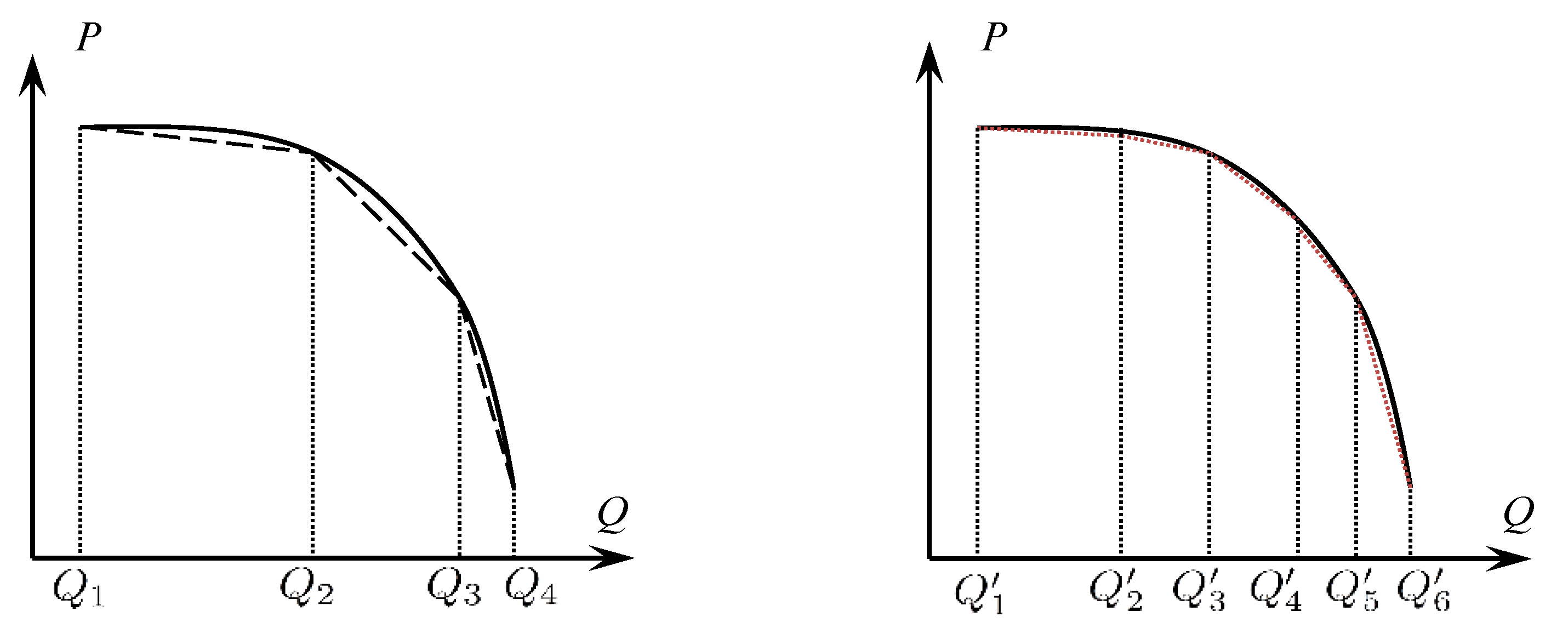
Three scenarios of quantity loss can be considered: (1) where the logistical function $Q_0{(c+d\exp (et+f))}^{-1}$ arises from quality evolution and the exponential function $Q_0\exp (-at+b)$ arises from quantity evolution; (2) where the exponential function $Q_0\exp (-at+b)$ is driven by quantity evolution; and (3) where the logistical function $Q_0{(c+d\exp (et+f))}^{-1}$ is driven by quantity evolution or quality evolution. If these scenarios are compared, it is apparent that a discount contract is an effective way to ensure market clearance and supply chain coordination with maximal profit. The duration, size, and point in time of discounts are crucial in this strategy. In this paper, discount size has been discussed by considering the loss of both quality and quantity.

6.1.3. A Universal Coordination Strategy for Multi-Stage Discounts

By analyzing other quantity losses with diverse decay functions, and comparing the corresponding results of the transitory optimal discount ratios of supermarkets and agricultural cooperatives, a hypothesis can be proposed: There is a universal law that can coordinate supply chains in all scenarios. If this is true, all supply chains coupled with diverse scenarios could be coordinated in a discount strategy that uses certain discount ratios. The main idea of the coordination strategy would be the same in all scenarios, but the corresponding parameters of discount ratios and times would vary. The next subsection will attempt to find this universal law.

It can also be concluded that the discount size in the centralized decision-making mode relies on fixed and drift terms, regardless of which loss function arises from exponential, logistical, mixed, or other types of distribution. For a multi-stage discount strategy, the fixed term of the supermarket’s discount ratio ${\displaystyle \sum _{n=1}^n{\left({\eta }_r^{n-1}\right)}^{*}}$ is

$$\frac{c}{2p_r}-\frac{U}{4p_r(\beta -\alpha )}+\frac{(2\theta -1)U}{4p_r(\beta +\alpha )}$$

(74)

while the drift term relies on the distribution properties of quantity and quality loss. After generalizing the results of the corresponding distribution, the drift term of the supermarket’s discount ratio is:

$$\frac{\gamma q_0}{p_r}{\displaystyle \sum _{n=1}^n\left[\frac{1}{\beta -\alpha }{\displaystyle {\int }_{T_{n-1}}^{T_w}Q(t)dt}-\frac{1}{\beta +\alpha }{\displaystyle {\int }_{T_{n-1}}^{T_n}Q(t)dt}\right]}$$

(75)

Equations (74) and (75) show that for supermarkets, if centralized decision making is invoked, the fixed term is independent of the distribution of quantity decay, but the drift term is. Further, whatever the distribution of quantity decay, the discount ratio in the multi-stage discount strategy will be determined by this fixed term, even if no quantity loss occurs. The fixed term of this discount ratio is decided by the unit cost of fresh agricultural produce from the agricultural cooperative; the price set by the supermarket in the traditional channel; the potential market size; the price sensitive coefficient of the channel price cross-elasticity coefficient between channels; and the market share in the traditional channel, which is described in Equation (74). There are, however, distinctions between scenarios that are driven by the properties of quantity decay and supply chain operation. The former is decided by the characteristics of the fresh agricultural produce, and the latter is controlled by supermarket prices in the traditional channel; the price-sensitive coefficient of a channel price cross-elasticity coefficient between channels; and the time intervals in a particular discount strategy. These two fractions form the drift term, as shown in Equation (75).

In agricultural cooperatives, the discount ratio also has two parts. The fixed term can be generalized as

$$\frac{c}{2p_r}-\frac{U}{4p_d(\beta -\alpha )}-\frac{(2\theta -1)U}{4p_d(\beta +\alpha )},$$

(76)

and the drift term as

$$\frac{\gamma q_0}{p_d}{\displaystyle \sum _{n=1}^n\left[\frac{1}{\beta -\alpha }{\displaystyle {\int }_{T_{n-1}}^{T_w}Q(t)dt}+\frac{1}{\beta +\alpha }{\displaystyle {\int }_{T_{n-1}}^{T_n}Q(t)dt}\right]}$$

(77)

If the decentralized decision-making mode is invoked, the discount ratio is similar to that of supermarkets. The fixed term is decided by the unit cost set by the agricultural cooperative; the price set by supermarkets in the traditional channel; the potential market size; the price-sensitive coefficient of the channel price cross-elasticity coefficient between channels; and the market share in the traditional channel, as described in Equation (76). The drift term is the same as that of the supermarket, which is affected by quantity decay and supply chain operation.

The universal law in the decentralized decision-making mode can be analyzed by using a similar method. In this case, the fixed term is the same as that of the centralized decision-making mode. The fixed term discount ratio for supermarkets and agricultural cooperatives would then be

$${\displaystyle \sum _{n=1}^n{\left({\eta }_r^{n-1}\right)}_{\mathrm{fixed}}^{*}}=\frac{\theta U}{2\alpha p_r}+\frac{\beta (1-\theta )U}{({\beta }^2-2{\alpha }^2)p_r}$$

(78)

and

$${\displaystyle \sum _{n=1}^n{\left({\eta }_d^{n-1}\right)}_{\mathrm{fixed}}^{*}}=\frac{(1-\theta )U\alpha }{\left({\beta }^2-2{\alpha }^2\right)p_d}$$

(79)

respectively. Similarly, the drift term discount ratio for supermarkets and agricultural cooperatives would be

$${\displaystyle \sum _{n=1}^n{\left({\eta }_r^{n-1}\right)}_{\mathrm{drift}}^{*}}=\frac{\gamma q_0}{p_r}{\displaystyle \sum _{n=1}^n\left[\frac{1}{\alpha }{\displaystyle {\int }_{T_{n-1}}^{T_w}Q(t)dt}+\frac{\alpha }{{\beta }^2-2{\alpha }^2}{\displaystyle {\int }_{T_{n-1}}^{T_n}Q(t)dt}\right]}$$

(80)

and

$${\displaystyle \sum _{n=1}^n{\left({\eta }_d^{n-1}\right)}_{\mathrm{drift}}^{*}}=\frac{\gamma q_0}{p_d}{\displaystyle \sum _{n=1}^n\left[\frac{\alpha }{{\beta }^2-2{\alpha }^2}{\displaystyle {\int }_{T_{n-1}}^{T_w}Q(t)dt}+\frac{\alpha }{{\beta }^2-2{\alpha }^2}{\displaystyle {\int }_{T_{n-1}}^{T_n}Q(t)dt}\right]}$$

(81)

respectively. If the sizes of these two discount ratios and decision-making modes are compared, it can be seen that the discount ratios are larger in the centralized mode, which reflects its advantage.

It can be concluded that Equations (74)–(77), (80) and (81) are the universal analytical expression of discount size. The former four equations fit the coordination strategy of decentralized decision making, and Equations (74), (76), (80) and (81) fit the centralized mode. In most cases, the universal coordination mechanism of multi-stage discounts with reasonable ratios will greatly benefit the supply chain and its node enterprises (Zhang et al., 2021 [42]).

Further, if Q(t) = 0, the optimal discount ratios would degenerate to the result proposed in [6,16,43]; if Q(t) = exp(a − bt), the optimal discount ratios would degenerate to the result proposed in [34]; if Q(t) is far larger than the normal quantity (i.e., it is a supernormal disruption, in which an extreme and sudden disruption occurs), the result calculated would match that shown in [16]. This proves Theorem 2 is correct.

6.1.4. Coordination within Agricultural Cooperatives

Agricultural cooperatives are composed of several families who work together, in order to generate more profit than they would working alone. In this kind of enterprise, effective management (including planning, organization, control and coordination) increases its benefits.

A question then arises: How can all families obtain reasonable profits under the condition of maximized cooperative payment? This problem can be described as a dynamic stochastic cooperative game model, which is complex to resolve. A solution can be obtained without losing accuracy, by solving two sequential problems: first, a corresponding optimal model of profit under certain constraints should be constructed (this should be a multi-objective optimization model, but whatever category of model is used, a corresponding optimal solution should be obtained); second, a reasonable profit distribution mechanism should be designed, to make sure all families are compensated fairly.

Because the first question is an optimization problem, no matter how complicated it is, it can be solved by invoking a fitness algorithm. The objective function of an agricultural cooperative is multi-faceted: maximum profit, sustainable production, and a healthy relationship with other enterprises in the supply chain are all considerations. The objective of an agricultural family is, however, relatively simple: maximum payment. A rational payment distribution can be determined by constructing a dynamic Shapley distribution vector, if the optimal payment of the cooperative and all possible coalitions are calculated. Because this problem is relatively simple, it was omitted from this paper.

6.2. Conclusions

The structure of a fresh agricultural produce supply chain is extremely complex. Three kinds of coordination are involved in its operation: that between the agricultural cooperative and the supermarket; that between traditional and E-commerce channels; and that between families in a cooperative. The former two focus on the conflict between the supermarket and the agricultural cooperative in the two channels, and the latter involves conflict within the cooperative. To resolve these conflicts, coordination between enterprises is key. After analysis, it can be concluded that the application of discounts is an effective coordination strategy. Further, the coordination of discounts in the centralized decision-making mode is more effective than under the decentralized mode. The paper then studied a scientific discount parameter.

According to supply chain operation and coordination, the supermarket encourages demand through discounts, and the agricultural cooperative gives discounts to promote the E-commerce channel but surrenders part of its profits to the supermarket in the traditional channel. Because the quantity of fresh agricultural produce decreases with time, however, and because market demand is determined by supply, the price, including the corresponding discount ratio, is difficult to ascertain. This paper introduced a multi-stage discount strategy, and calculated each discount ratio coupled with its corresponding stage. If the quantity decays as in Equations (1) and (2), corresponds to the loss of quantity and quality, respectively, and if the decentralized decision-making mode is introduced, the optimal discount for the supermarket is described in Equation (71), and the discount for the agricultural cooperative in Equation (70). If centralized decision making is used but all other conditions remain the same, the optimal discounts for the supermarket and agricultural cooperative are decided by Equations (72) and (73), respectively. The centralized decision-making mode is superior to the decentralized mode in terms of coordination effect.

There are, however, other kinds of quantity loss in fresh agricultural produce that have diverse functions determined by the product’s physical properties and biochemical characteristics. This paper discussed the loss function of exponential and logistical decay, and found that whatever the nature of quantity loss, there is a universal function that describes the discount ratio. It then divided the discount behaviors into two aspects: fixed term (which is independent of changes to quantity and quality); and drift term (which is dependent on these changes). In the decentralized decision-making mode, the fixed term of supermarket discounts is given in Equation (78), and the drift term in Equation (80); and the fixed term of the agricultural cooperative discount is given in Equation (79), and the drift term in Equation (81). In the centralized decision-making mode, the fixed term of supermarket discounts is given in Equation (74), and the drift term in Equation (75); and the fixed term of agricultural cooperative discounts is given in Equation (76), and the drift term in Equation (77).

If this universal conclusion is analyzed, it is found that, regardless of what kind of quantity loss occurs, whether decentralized or centralized decision making is selected, or whether the supermarket’s or agricultural cooperative’s discount ratio is considered, the fixed term discount relies on the market share in the traditional channel; the potential market size; the retail price; the price sensitive coefficient of the channel; and the cross-elasticity coefficient of prices between channels. The drift term discount relies on the initial quantity of fresh agricultural produce in the supply chain; the retail price; the price-sensitive coefficient of the channel cross-elasticity coefficient of price between different channels, and property of quantity loss.

Another problem cannot be discussed: In the mapping between profit π and discount time n, it can be concluded from the demand Equations (46) and (47), and the profit Equations (60) and (65), that there is a positive correlation between π and n, such that the profit π is positively correlated with the discount time n. This is because long discount times decrease the difference between demand and supply, which in turn decreases the cost of disposing of a superfluous supply of fresh agricultural produce. Unfortunately, the discount cost cannot be analyzed using the demand Equations (46) and (47), or the profit Equations (60) and (65), which makes the positive correlation between n and π unacceptable. Each discount can produce some degree of cost or loss, and this should be added to the profit equations. The mapping between profit π and discount time n is therefore very complex, and probably a non-negative correlation. Further, if the discount times is too large, consumers could play a larger role in setting prices in the supply chain, and each further discount would increase the difficulty of management of the supply chain, thereby decreasing the profits of the supermarket and/or agricultural cooperative. For this reason, moderate discount times should be considered.

The dynamic discount ratio ${\eta }_r^{\mathit{i*}}$ and ${\eta }_d^{\mathit{i*}}$ at discount stage i are given as discussed, which raises another, more interesting, question: How long should discount stages be to yield maximum profit, supply chain coordination and market clearing? To ascertain this, the profits of the agricultural cooperative, supermarket and supply chain should be considered, and the relationship between profit π and discount time n should be analyzed. Discount time is therefore an important parameter in the discount coordination strategy, and it will be studied in the next paper.

References

1. Clark, L.F.; E Hobbs, J. Informational barriers, quality assurance and the scaling up of complementary food supply chains in Sub-Saharan Africa. Outlook Agric. 2018, 47, 11–18. [Google Scholar] [CrossRef] [Green Version]
2. Vernier, C.; Loeillet, D.; Thomopoulos, R.; Macombe, C. Adoption of ICTs in Agri-Food Logistics: Potential and Limitations for Supply Chain Sustainability. Sustainability 2021, 13, 6702. [Google Scholar] [CrossRef]
3. Tian, X.; Niu, M.; Zhang, W.; Li, L.; Herrera-Viedma, E. A novel todim based on prospect theory to select green supplier with q-rung orthopair fuzzy set. Technol. Econ. Dev. Econ. 2020, 27, 284–310. [Google Scholar] [CrossRef]
4. Walker, M.J.; Burns, D.T.; Elliott, C.T.; Gowland, M.H.; Mills, E.N.C. Is food allergen analysis flawed? Health and supply chain risks and a proposed framework to address urgent analytical needs. Analyst 2015, 141, 24–35. [Google Scholar] [CrossRef] [Green Version]
5. Magalhães, V.S.; Ferreira, L.M.D.; Silva, C. Using a methodological approach to model causes of food loss and waste in fruit and vegetable supply chains. J. Clean. Prod. 2020, 283, 124574. [Google Scholar] [CrossRef]
6. Siddh, M.M.; Soni, G.; Jain, R.; Sharma, M.K.; Yadav, V. Agri-fresh food supply chain quality (AFSCQ): A literature review. Ind. Manag. Data Syst. 2017, 117, 2015–2044. [Google Scholar] [CrossRef] [Green Version]
7. Xu, X.; Lin, Z.; Li, X.; Shang, C.; Shen, Q. Multi-objective robust optimisation model for MDVRPLS in refined oil distribution. Int. J. Prod. Res. 2021. [Google Scholar] [CrossRef]
8. Smith, R.D. Propagation of Cascades in Complex Networks: From Supply Chains to Food Webs. arXiv 2011, arXiv:1103.4983. [Google Scholar]
9. Nosratabadi, S.; Mosavi, A.; Lakner, Z. Food Supply Chain and Business Model Innovation. Foods 2020, 9, 132. [Google Scholar] [CrossRef] [PubMed] [Green Version]
10. Xu, N.; Huang, Y.F.; Weng, M.W.; Do, M.H. New Retailing Problem for an Integrated Food Supply Chain in the Baking Industry. Appl. Sci. 2021, 11, 946. [Google Scholar] [CrossRef]
11. Huang, X.; Yang, S.; Wang, Z. Optimal pricing and replenishment policy for perishable food supply chain under inflation. Comput. Ind. Eng. 2021, 158, 107433. [Google Scholar] [CrossRef]
12. Gaggero, M.; Tonelli, F. A two-step optimization model for the distribution of perishable products. Networks 2020, 78, 69–87. [Google Scholar] [CrossRef]
13. Zheng, Q.; Ieromonachou, P.; Fan, T.; Zhou, L. Supply chain contracting coordination for fresh products with fresh-keeping effort. Ind. Manag. Data Syst. 2017, 117, 538–559. [Google Scholar] [CrossRef]
14. Liu, P.; Long, Y.; Song, H.-C.; He, Y.-D. Investment decision and coordination of green agri-food supply chain considering information service based on blockchain and big data. J. Clean. Prod. 2020, 277, 123646. [Google Scholar] [CrossRef]
15. Moon, I.; Sarmah, S.; Saha, S. The impact of online sales on centralised and decentralised dual-channel supply chains. Eur. J. Ind. Eng. 2018, 12, 67. [Google Scholar] [CrossRef]
16. Mitchell, R.; Maull, R.; Pearson, S.; Brewer, S.; Collison, M. The impact of COVID-19 on the UK fresh food supply chain. arXiv 2020, arXiv:2006.00279. [Google Scholar]
17. Kramer, M.P.; Bitsch, L.; Hanf, J. Blockchain and Its Impacts on Agri-Food Supply Chain Network Management. Sustainability 2021, 13, 2168. [Google Scholar] [CrossRef]
18. Saurabh, S.; Dey, K. Blockchain technology adoption, architecture, and sustainable agri-food supply chains. J. Clean. Prod. 2020, 284, 124731. [Google Scholar] [CrossRef]
19. Kamilaris, A.; Fonts, A.; Prenafeta-Boldύ, F.X. The rise of blockchain technology in agriculture and food supply chains. Trends Food Sci. Technol. 2019, 91, 640–652. [Google Scholar] [CrossRef] [Green Version]
20. Saha, S. Channel characteristics and coordination in three-echelon dual-channel supply chain. Int. J. Syst. Sci. 2014, 47, 740–754. [Google Scholar] [CrossRef]
21. Saha, S.; Nielsen, I. Strategic Integration Decision under Supply Chain Competition in the Presence of Online Channel. Symmetry 2020, 13, 58. [Google Scholar] [CrossRef]
22. Xu, X.; Wang, C.; Zhou, P. GVRP considered oil-gas recovery in refined oil distribution: From an environmental perspective. Int. J. Prod. Econ. 2021, 108078. [Google Scholar] [CrossRef]
23. Xu, X.; Lin, Z.; Zhu, J. DVRPLS with Variable Neighborhood Region in Refined Oil Distribution. Ann. Oper. Res. 2020, 309, 663–687. [Google Scholar] [CrossRef]
24. Ezzeddine, B.; Abdellatif, B.; Mounir, B. An Agent-based framework for cooperation in Supply Chain. arXiv 2012, arXiv:1210.3375. [Google Scholar]
25. Kollia, I.; Stevenson, J.; Kollias, S. AI-Enabled Efficient and Safe Food Supply Chain. Electronics 2021, 10, 1223. [Google Scholar] [CrossRef]
26. Kurnia, S.; Hill, S.; Rahim, M.M.; Larsen, K.; Braun, P.; Samson, D. Open Food Network: The Role of ICT to Support Regional Food Supply Chains in Australia. arXiv 2016, arXiv:1606.01456. [Google Scholar]
27. Tabrizi, S.; Ghodsypour, S.H.; Ahmadi, A. Modelling three-echelon warm-water fish supply chain: A bi-level optimization approach under Nash–Cournot equilibrium. Appl. Soft Comput. 2018, 71, 1035–1053. [Google Scholar] [CrossRef]
28. Chen, X.; Wu, S.; Wang, X.; Li, D. Optimal pricing strategy for the perishable food supply chain. Int. J. Prod. Res. 2018, 57, 2755–2768. [Google Scholar] [CrossRef] [Green Version]
29. Zhai, Y.; Han, G. The effect of the inspection information sharing policy on quality-oriented food production in online commerce. Manag. Decis. Econ. 2021, 43, 84–96. [Google Scholar] [CrossRef]
30. Zhu, Q.; Li, X.; Zhao, S. Cost-sharing models for green product production and marketing in a food supply chain. Ind. Manag. Data Syst. 2018, 118, 654–682. [Google Scholar] [CrossRef]
31. Tang, R.; Li, Q.; Peng, Y. Market clearing strategy in dual channel of fresh agricultural products considering quality loss. Syst.Eng.—Theory Pract. 2018, 38, 2542–2555. [Google Scholar] [CrossRef]
32. Zhang, X.; Yuan, X. Reward-penalty Mechanism for Reverse Supply Chain Network with Asymmetric Information and Carbon Emission Constraints. arXiv 2017, arXiv:1702.07638. [Google Scholar]
33. Hu, J.Y.; Zhang, J.; Mei, M.; Yang, W.; Shen, Q. Quality control of a four-echelon agri-food supply chain with multiple strategies. Inf. Processing Agric. 2019, 6, 425–437. [Google Scholar] [CrossRef]
34. Tran, T.H. Critical Factors and Enablers of Food Quality and Safety Compliance Risk Management in the Vietnamese Seafood Supply Chain. Int. J. Manag. Value Supply Chains 2018, 9, 1–20. [Google Scholar] [CrossRef]
35. Neubert, G.; Ouzrout, Y.; Bouras, A. Collaboration and integration through information technologies in supply chains. Int. J. Technol. Manag. 2004, 28, 259. [Google Scholar] [CrossRef]
36. Singh, A.; Mishra, N.; Ali, S.I.; Shukla, N.; Shankar, R. Cloud computing technology: Reducing carbon footprint in beef supply chain. Int. J. Prod. Econ. 2015, 164, 462–471. [Google Scholar] [CrossRef] [Green Version]
37. Stranieri, S.; Orsi, L.; Banterle, A.; Ricci, E.C. Sustainable development and supply chain coordination: The impact of corporate social responsibility rules in the European Union food industry. Corp. Soc. Responsib. Environ. Manag. 2018, 26, 481–491. [Google Scholar] [CrossRef]
38. Belkhatir, M.; Bala, S.; Belkhatir, N. Business process re-engineering in supply chains examining the case of the expanding halal industry. arXiv 2020, arXiv:2004.09796. [Google Scholar]
39. Suhail, S.; Hussain, R.; Khan, A.; Hong, C.S. Orchestrating product provenance story: When IOTA ecosystem meets electronics supply chain space. Comput. Ind. 2020, 123, 103334. [Google Scholar] [CrossRef]
40. Inoue, H.; Murase, Y.; Todo, Y. Lockdowns need geographic coordination because of propagation of economic effects through supply chains. arXiv 2021, arXiv:2101.01679. [Google Scholar] [CrossRef]
41. Tominac, P.A.; Zavala, V.M. Economic Properties of Multi-Product Supply Chains. arXiv 2020, arXiv:2006.03467. [Google Scholar] [CrossRef]
42. Zhang, J.; Brintrup, A.; Calinescu, A.; Kosasih, E.; Sharma, A. Supply Chain Digital Twin Framework Design: An Approach of Supply Chain Operations Reference Model and System of Systems. arXiv 2021, arXiv:2107.09485. [Google Scholar]
43. Tominac, P.A.; Zhang, W.; Zavala, V.M. Spatio-temporal economic properties of multi-product supply chains. Comput. Chem. Eng. 2022, 159, 107666. [Google Scholar] [CrossRef]
Figure 1. The fresh agricultural produce supply chain and discount coordination process.
Sustainability 14 02174 g001
Figure 2. The change of demand function with price.
Sustainability 14 02174 g002
Figure 3. Attractor stability.
Sustainability 14 02174 g003
Figure 4. The demand function of fresh agricultural produce and the effect of multi-stage discounts.
Sustainability 14 02174 g004
Figure 5. Multi-stage discount coordination in the fresh agricultural produce supply chain.
Sustainability 14 02174 g005