An Air Quality Modeling and Disability-Adjusted Life Years (DALY) Risk Assessment Case Study: Comparing Statistical and Machine Learning Approaches for PM_2.5 Forecasting

Abstract

Despite Central and Northern Asia having several cities sharing a similar harsh climate and grave air quality concerns, studies on air pollution modeling in these regions are limited. For the first time, the present study uses multiple linear regression (MLR) and a random forest (RF) algorithm to predict PM_2.5 concentrations in Astana, Kazakhstan during heating and non-heating periods (predictive variables: air pollutant concentrations, meteorological parameters). Estimated PM_2.5 was then used for Disability-Adjusted Life Years (DALY) risk assessment. The RF model showed higher accuracy than the MLR model (R² from 0.79 to 0.98 in RF). MLR yielded more conservative predictions, making it more suitable for use with a lower number of predictor variables. PM₁₀ and carbon monoxide concentrations contributed most to the PM_2.5 prediction (both models), whereas meteorological parameters showed lower association. Estimated DALY for Astana’s population (2019) ranged from 2160 to 7531 years. The developed methodology is applicable to locations with comparable air pollution and climate characteristics. Its output would be helpful to policymakers and health professionals in developing effective air pollution mitigation strategies aiming to mitigate human exposure to ambient air pollutants.

1. Introduction

Developments in industrial sectors, increased private transportation, exploitation of resources, and population growth have been the main contributors to the increase in the concentrations of ambient air pollutants in urban and rural areas of developing countries [1]. Atmospheric particulates can be directly emitted from intensive traffic, industrial combustion processes, and domestic coal burning [1,2,3] as well as from chemical reactions among various pollutants in the lower atmosphere as secondary pollutants (e.g., VOCs, SO₂, NO₂) [4]. Subsequently, particulate matter (PM) and gaseous pollutants (e.g., CO, SO₂, and NOx) may pose a serious health risk to the exposed population, particularly when they exceed the maximum allowable concentrations [5].

According to the World Health Organization (WHO), more people are affected by PM in comparison to other air pollutants [5]. Several studies have established links between increased PM concentrations and higher morbidity and mortality rates (e.g., [3,4,6,7,8]). It is estimated that exposure to PM in ambient air is the cause of approximately 7 million deaths annually worldwide [5]). Moreover, PM fractions of smaller particles (e.g., PM_2.5, PM_0.1) are suggested to pose a greater health risk due to their ability to penetrate the circulatory system through lung alveoli and terminal bronchioles. Gaseous ambient air pollutants also contribute to the degradation of air quality and human exposure increases the risk of respiratory conditions (e.g., asthma, bronchitis, airway irritation, and pulmonary edema) [9]. Therefore, effective air quality monitoring is imperative to mitigate the exposure of local populations to atmospheric contaminants in urban areas, such as Astana, Kazakhstan, with increasing population, high traffic activity, and poor air quality.

Astana is in northern Kazakhstan and heavily relies on coal-fired power plants (marked as CHP-1 and CHP-2 in Figure 1) to fulfill extensive energy demands, particularly during extremely cold winter times [10]. Highly elevated concentrations of various atmospheric pollutants (e.g., PM, SO₂, formaldehyde) in the city during the heating period (October–April) were attributed to increasing amounts of emissions from residential cheap coal burning, industrial heat supply plants, and heavy traffic [10]. Currently, only a few air pollution monitoring stations collect PM_2.5 and gaseous pollutants concentrations in Astana, which makes air quality assessment in the region a challenging and often incomplete task. Thus, predicting ambient pollutant concentrations may be an efficient means for local air quality monitoring control.

Multiple Linear Regression (MLR) analysis may be used to associate atmospheric concentrations of the ambient air pollutants with parameters that affect their formation and distribution, including meteorological characteristics and other atmospheric parameters [1,11,12]. The technique has become a widely utilized forecasting tool due to its ease of implementation and lesser computing demand [13]. In various studies, MLR demonstrated a good prediction potential while focusing on the investigation of different atmospheric phenomena (e.g., prediction of atmospheric pollutants concentrations as well as precipitation and evapotranspiration rates, etc.) with insufficient data (e.g., [11,14,15]).

There have been notable developments in implementing sensing technologies involving newer technology such as the internet of things and machine learning to indoor and outdoor air quality monitoring/exposure assessment (e.g., [16,17]), albeit low-cost and novel technology has yet to be widely adopted. An emerging, promising tool used in air quality modeling is machine learning (ML), which enables predicting nonlinear data effectively. The use of artificial intelligence (AI) for forecasting air pollutant concentrations comprises of the generation of an ML model, an input dataset (which will be used for model training and testing), and model validation. One technique for the development of an ML-based model for PM_2.5 concentration forecasting is the random forest (RF) algorithm. RF has been cited as a fast and cost-efficient algorithm that may be able to model air quality more accurately than other ML techniques (e.g., artificial neural networks (ANN), XGBoost, support vector regression (SVR)) [18,19,20,21,22]. Furthermore, the RF algorithm was specifically selected to address the data collinearity issue, which may occur due to possible strong correlation between PM_2.5 and PM₁₀ concentrations. This feature of the RF model was successfully utilized in reducing the risk of obtaining biased results during the data classification [23].

A quality approach to PM_2.5 concentration forecasting is particularly valuable to regions with limited data on PM_2.5 concentrations. Air quality modeling using novel ML techniques such as RF could prove useful in these regions with scarce data. An example of such regions is Central and Northern Asia, where studies on air pollution modeling are sparse. To the authors’ best knowledge, a comparison between conventional statistical modeling and ML algorithms has not yet been employed for this region, with several urban areas sharing similar meteorological and topographic characteristics. These regions contain numerous cities sharing a similar harsh climate and severe air quality concerns, along with limited monitoring data. Employing relatively well-established (e.g., MLR) in combination with more novel (e.g., RF) prediction tools to overcome the issue of limited monitoring data for these regions has not yet been suggested. Moreover, a case of health risk assessment (HRA) using predicted concentrations would not only serve as a practical and replicable public health estimation tool, but may also provide evidence to help assist the issue of adverse health outcomes following exposure to air pollutants. More specifically, suggested HRA as a tool could assist health professionals, policymakers, and governmental institutions to make proactive decisions in air pollution mitigation strategies via a rapid comparison of associated costs and health benefits.

The objectives of the present study are (1) to analyze the annual and seasonal variation in PM_2.5, PM₁₀, and gaseous pollutants (CO, NO₂, NO, and SO₂) in Astana, Kazakhstan; (2) to utilize MLR and RF algorithm to predict PM_2.5 and compare the model performance (3); and to assess human health risks via a DALY risk assessment for the population of Astana using predicted PM_2.5 concentration values.

2. Methodology

2.1. Study Area

Astana, the capital city of Kazakhstan, is located in the north-central region of the country (51°10′ N, 71°26′ E) and at 347 m above sea level (Figure 1). The area of the capital city is 722 km², which is a part of the dry steppe zone. It has a continental climate with characteristic climate variability and well-defined seasons [24]. It is characterized by sharp ambient temperature fluctuations and the formation of weather anomalies such as episodes of severe frosts, thaws, and rains in winter along with extreme heat and frost in summer [24]. The annual average temperature of Astana is 3.5 °C, and the average wind speed is 3.9 m/s. The warmest month is July, with an average temperature of +20.4 °C, whereas the coldest month is January, with an average temperature of −14.2 °C [25].

According to data from the Bureau of National Statistics [26], the total population of Astana was 1,047,966 people in 2019, where population density was high and varied among four districts of the city, namely Esil (517 people/km²), Almaty (1986 people/km²), Baikonur (1180 people/km²), and Saryarka (4770 people/km²). Both coal-fired power plants are located in Baikonur district (Figure 1).

2.2. Data Collection

The data were obtained from the National Air Quality Monitoring Network (NAQMN) of the National Hydrometeorological Service of Kazakhstan, “Kazhydromet.” The average daily pollutant concentrations from two monitoring stations (S5 and S6) (Figure 1) throughout 2019 have been utilized. These air pollution monitoring stations perform ongoing automatic measurements of pollutant concentrations. The obtained data contained hourly measurements of PM_2.5, PM₁₀, SO₂, CO, NO₂, and NO concentrations. The meteorological parameters used in the present study were temperature (T), atmospheric pressure (P), relative humidity (RH), wind direction (WD), and wind speed (WS). Average daily data were separated into two periods (i.e., heating (October–April) and non-heating (May–September)).

2.3. Statistical Analyses

The data sets were not normally distributed; thus, Spearman’s correlation test was conducted to calculate the correlation coefficient (r) between PM_2.5 concentration and independent variables (PM₁₀, SO₂, CO, NO₂, NO, T, P, RH, WD, and WS). MLR was performed to determine the relationship between dependent (PM_2.5) and independent variables (gaseous pollutant concentrations, meteorological parameters). Before constructing the regression models, several assumptions were verified, including the linear relationship between the dependent and independent variables, absence of multicollinearity, multivariate normality, and homoscedasticity of residuals [1,2,27]. Model validation was performed using statistical methods of evaluating the model equation’s performance, including Variance Inflation Factor (VIF), Root-Mean-Squared Error (RMSE), Mean Absolute Error (MAE), Normalized Absolute Error (NME), Index of Agreement (IA), Prediction Accuracy (PA), and Coefficient of Determination (R²). Formulas along with desired values for model evaluation parameters have been described elsewhere [1,11]. Statistical analysis was performed using Stata 14.2 by StataCorp^® software.

2.4. Machine Learning

The RF algorithm was implemented to develop an ML-based model for PM_2.5 concentration forecasting. Training and testing datasets were obtained from the same data used for the construction of the MLR model. In the present study, 80% of the data were used for model training and the remaining 20% were used for model testing. This ratio for data separation was employed in the present model due to the large number (10) of predictor variables and the size of the data available (n = 7912 for S5, n = 6931 for S6) for concentration forecasting [18,28]. Python was used for the construction of the RF model and the evaluation of its performance. Forecast accuracy and overall model performance were assessed using the testing dataset, via the same indices used for the MLR model performance validation. Additionally, a 10-fold cross-validation (CV) was performed to evaluate the performance of the training set by dividing it into training and validation subsets ten times with subsequent model performance analysis.

2.5. Human Health Risk Assessment

AIRQ+ software has been developed by the WHO Regional Office for Europe to quantify the impact of air pollution and the health burden associated with a particular pollutant [29,30]. In the present study, human health risk assessment (HHRA) was conducted using ‘Life Table Evaluation module’ in AIRQ+ software [30] to determine the DALY associated with PM_2.5 inhalation exposure in Astana. DALY represents the years of life lost due to early death and/or diseases attributed to a particular pollutant exposure [31,32,33,34]:

DALY = YLL + YLD

(1)

where YLL is Years of Life Lost due to premature death and YLD is Years of Life Lost due to Disability. Data on respiratory and cardiovascular mortality and morbidity cases of the study population were used for the calculation of the YLD, and YLL was retrieved from the national database on the socio-economic status of the Republic of Kazakhstan [26]. A mean pollutant (PM_2.5) concentration and the exposure-response coefficient (β) for all-cause mortality data from previous studies [30,35,36] were imputed to calculate the relative risk (RR):

$$\mathrm{RR}={\mathrm{e}}^{\mathsf{\beta }\times \Delta \mathrm{x}}$$

(2)

where Δx is the difference between the observed PM_2.5 concentrations and the concentration at which PM_2.5 exposure is assumed to result in adverse health effects. AIRQ+ then employs the RR value to determine the YLL for several age groups. YLD values were calculated [32]:

$$\mathrm{YLD}={{\displaystyle \sum }}_{\mathrm{i}}\left({\mathrm{Mortality} \mathrm{cases}}_{\mathrm{i}}\times {\mathrm{Disability} \mathrm{weight}}_{\mathrm{i}}\times {\mathrm{PAF}}_{\mathrm{i},\mathrm{g}}\right)$$

(3)

where, Disability weight_i is unique to each disease or disability group that denotes its disability level, and PAF_i,g is the population attributable fraction of disease or disability group i for a population group g, which is calculated as follows [32,33]:

$${\mathrm{PAF}}_{\mathrm{i},\mathrm{g}}=\frac{{\mathrm{Population} \mathrm{proportion}}_{\mathrm{g}}\times \left({\mathrm{RR}}_{\mathrm{i},\mathrm{g}}-1\right)}{{\mathrm{Population} \mathrm{proportion}}_{\mathrm{g}}\times \left({\mathrm{RR}}_{\mathrm{i},\mathrm{g}}-1\right)+1}$$

(4)

where Population proportion_g is the fraction of the population exposed to elevated PM_2.5 concentrations in a population group g [32,33].

3. Results and Discussion

3.1. PM_2.5 Pollution Profile

Table 1. Annual and seasonal variations in the concentration of PM_2.5 (µg/m³) in 2019.

	S5			S6
	Annual	Heating	Non- Heating	Annual	Heating	Non- Heating
Mean	14.5	18.1	10.4	58.0	77.2	38.7
SD	26.1	33.7	11.1	75.1	93.6	41.8
Range (25th–95th)	(5.60–43.6)	(5.90–54.2)	(5.30–29.5)	(21.8–186)	(26.6–242)	(19.7–107)
Min	0	0	0	5.7	5.7	7.1
Max	824	824	126	1086	1086	985

demonstrates annual and periodic (i.e., during heating (October–April) and non-heating periods (May–September)) variation in concentration of PM_2.5 in 2019. The annual average concentration of PM_2.5 in 2019 was higher at S6 compared to S5 (58.0 and 14.5 µg/m³ respectively), which may be attributed to its proximity to coal-fired power plants and heavy traffic areas. Both S5 and S6 annual average PM_2.5 concentrations exceeded the WHO maximum permissible annual concentration (5 µg/m³) [30].

It is worth noting that the average heating period PM_2.5 concentrations were higher than the non-heating concentrations for both stations. The average heating period concentrations peaked in January (Figure 2), during which the highest concentration of PM_2.5 was 1086 µg/m³ (S6). The average concentration of PM_2.5 increased almost two-fold during the heating period at each monitoring station, which could be attributed to increased emissions from residential furnaces, higher rates of particulate resuspension, and atmospheric reactions resulting in the formation of PM_2.5 [37].

In-week changes in PM_2.5 varied for S5 and S6, demonstrating peaks of 70 µg/m³ on Saturday at S5 and 20 µg/m³ on Thursday at S6. Comparable trends in the variation of PM_2.5 concentrations have been present in other studies [38,39,40]. The hourly concentrations of PM_2.5 varied throughout the day such that they peaked at midnight and then steadily decreased until around 16:00 at both stations (Figure 3). The observed peak of PM_2.5 at midnight could be attributed to the temperature drop that may combine with inversion conditions, resulting in higher accumulation of pollutants [41]. A similar “W-shaped” pattern in hourly PM_2.5 concentrations has been observed in some studies (e.g., [42,43,44]). Such large fluctuations between daytime and nighttime concentrations may also be associated with the atmospheric stability that occurs during night hours [43].

3.2. Pollution Profiles for PM₁₀, CO, NO, NO₂, and SO₂

The annual mean concentration of PM₁₀ during the study year was within the WHO annual limit (15 µg/m³) at S5 but not at S6 (

Table 2. Periodic variations in ambient pollutant concentrations (µg/m³) in 2019.

S5
	Annual			Heating			Non-Heating
Air Pollutant	Mean	SD	Range (25th–95th)	Mean	SD	Range (25th–95th)	Mean	SD	Range (25th–95th)
PM10	3.12	3.8	(1.5–7.3)	2.73	2.23	(1.4–5.7)	3.80	3.82	(1.9–9.5)
CO	485	3006	(34.1–931)	250	549	(35.2–1011)	745	4330	(33.2–838)
NO	29.9	33.8	(2.4–88.2)	25.3	32.0	(1–83.9)	35.1	35	(12.5–94.7)
NO2	25.8	25.8	(1.2–32.4)	10.3	26.7	(1.2–37.1)	9.60	24.7	(1.6–23.5)
SO2	19.7	18.6	(7.9–58.1)	20.9	20.7	(8.00–63.7)	18.3	15.8	(7.8–45)
S6
	Annual			Heating			Non-Heating
Air Pollutant	Mean	SD	Range (25th–95th)	Mean	SD	Range (25th–95th)	Mean	SD	Range (25th–95th)
PM10	60.3	75.9	(23.4–190)	79.1	94.5	(27.9–244)	41.4	43.4	(21.3–114)
CO	630	495	(323–1553)	742	540	(405–1726)	518	416	(269–1245)
NO	9.01	21.0	(1.10–41.1)	9.17	18.9	(1.10–42.5)	8.86	22.8	(1.10–37.1)
NO2	39.7	27.1	(17.2–81.0)	40.7	23.9	(20.6–77.6)	38.7	30.0	(15.1–88.5)
SO2	125	320	(2.90–949)	239	422	(7.70–1114)	10.3	10.9	(2.90–28.0)

). The average PM₁₀ concentrations during the heating season were two-fold higher than in the non-heating period in S6 (79.1 µg/m³ vs. 41.4 µg/m³). These results would be interpreted as concerning due to the fact that human exposure to elevated PM₁₀ concentrations contributes to higher cardiorespiratory hospital admissions among the elderly population and to morbidity associated with chronic bronchitis [4,39]. The annual mean NO concentration at S5 and S6 in 2019 did not exceed the EU maximum permissible limit for NO_x (30 µg/m³). Furthermore, the average annual concentration of NO₂ did not exceed WHO air quality guidelines (40 µg/m³) at S5 and S6. The highest average NO₂ concentration was during the heating period at S6 (40.7 µg/m³, range: 20.6–77.6 µg/m³). The annual average concentration of SO₂ exceeded the National Air Quality Standards maximum permissible concentration for the residential area (60 µg/m³) [45] at S6 (125 µg/m³, range: 2.90–949 µg/m³). The heating period at S6 was characterized by episodes of very high SO₂ concentrations, a mean of 239 µg/m³ and ranging from 7.70 µg/m³ to 1114 µg/m³. S6 recorded an increase in SO₂ levels in November and December, with concentrations up to 1000 µg/m³. These results would also be interpreted as concerning due to the fact that SO₂ is highly soluble and thus could be readily absorbed in the respiratory tract; this subsequently causes airway inflammation that results in coughing, secretion of mucus, and chronic bronchitis (particularly dangerous to vulnerable populations (e.g., asthmatic group)) [46,47].

The highest annual mean concentration of CO was observed at S6 (630 µg/m³) and ranged from 323 µg/m³ to 1553 µg/m³ (Table 2). The annual average concentration of CO at S5 was lower, from 35 to 931 µg/m³ with a mean of 338 µg/m³. The mean as well as maximum values from S5 and S6 greatly exceed the daily maximum permissible level for CO according to the Kazakhstani standards (60 µg/m³) [48]. It is worth noting that episodes of extremely high concentrations of CO were recorded at S6 in September, peaking at 30,000 µg/m³. This is another concerning observation as chronic CO poisoning could result in adverse neurological symptoms such as cognitive impairments, movement disorders, speech impairment, and mood disturbances, particularly affecting population groups working in the transportation sector as well as traffic wardens and garage/tunnel workers [47].

3.3. Correlation between PM_2.5, Atmospheric Variables, and Meteorological Parameters

For atmospheric pollutants, positive correlations were found between PM_2.5 and PM₁₀, SO₂, CO, NO₂, NO, P, and RH; negative correlations were present between PM_2.5, WS, and T (

Table 3. Correlation coefficients (r) between PM_2.5, selected atmospheric pollutants, and meteorological parameters.

		S5						S6
		Heating			Non-Heating			Heating			Non-Heating
Parameters Correlated with PM2.5		r	Significance	Sample Size	r	Significance	Sample Size	r	Significance	Sample Size	r	Significance	Sample Size
Pollutant concentrations	PM10	0.12	0.096	188	0.76	<0.001	165	0.99	<0.001	160	0.99	<0.001	157
	SO2	0.03	0.716	188	0.23	0.003	165	−0.09	0.239	160	−0.02	0.758	157
	CO	0.87	<0.001	188	−0.17	0.025	165	0.87	<0.001	160	0.62	<0.001	157
	NO2	0.48	<0.001	188	0.17	0.031	165	0.55	<0.001	160	0.18	0.023	157
	NO	0.49	<0.001	188	0.47	<0.001	165	0.48	<0.001	160	0.28	<0.001	157
Meteorological Parameters	T	−0.45	<0.001	188	0.23	0.003	165	−0.47	<0.001	160	0.01	0.868	157
	P	0.23	0.002	188	0.05	0.528	165	0.36	<0.001	160	0.24	0.003	157
	RH	0.10	0.161	188	−0.16	0.037	165	0.03	0.697	160	0.01	0.869	157
	WD	−0.35	<0.001	188	−0.16	0.044	165	−0.61	<0.001	160	−0.39	<0.001	157
	WS	−0.38	<0.001	188	−0.17	0.028	165	−0.15	0.069	160	0.13	0.119	157

).

A high correlation (r = 0.99) was present between PM_2.5 and PM₁₀ in both heating and non-heating periods at S6. A similar high correlation (r = 0.76) between the aforementioned parameters was observed solely for the non-heating period at S5. A high correlation (r = 0.87 for S5 and S6) between PM_2.5 and CO, and a moderate correlation (0.30 < r < 0.80) between PM_2.5 and nitrogen gasses were present during the heating period at both stations. Finally, T, WS, and WD had a moderate but negative correlation with PM_2.5 during the heating period. These results indicate possible common origins of PM and other air pollutants. Similarly, as expected, more severe air pollution episodes could be associated with episodes of lower T (resulting in higher heating activity) and WD (weaker dispersion/mixing). Previous studies reported similar results regarding correlation between PM (PM_2.5 and PM₁₀) and gaseous pollutants (e.g., CO, NO_2, and SO₂) as well as for meteorological parameters, including atmospheric and dew point temperatures as well as WD (e.g., by [1,27]).

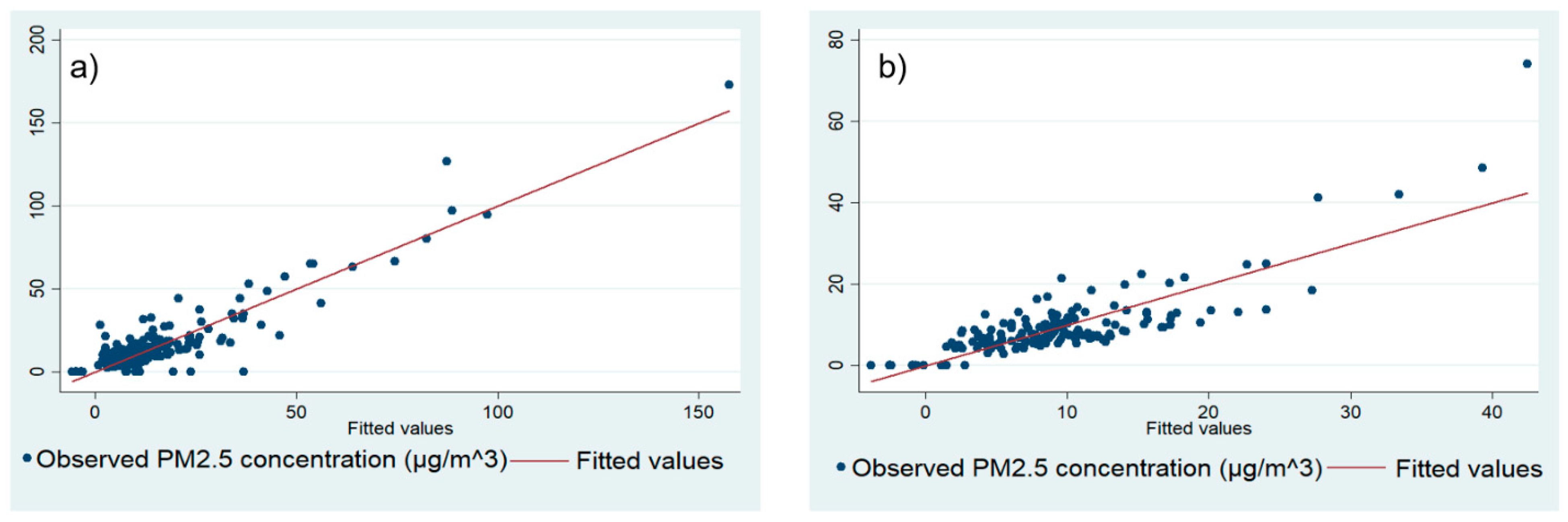
3.4. Multiple Linear Regression Predictive Models

Four predictive models for PM_2.5 concentrations have been established for S5 and S6 (i.e., for heating and non-heating periods) utilizing air pollution data and meteorological parameters via the multiple linear regression (MLR) equation. The MLR equation for forecasting PM_2.5 concentrations (

Table 4. MLR equation for PM_2.5 forecasting for 2019 air pollution monitoring data (S5 and S6).

	Model	VIF
S5
Heating	PM2.5 (µg/m3) = (−5.75) + 0.29 (PM10) (µg/m3) + 1.00 (CO) (µg/m3) − 0.13 (NO2) (µg/m3)	(1.04–1.63)
Non-heating	PM2.5 (µg/m3) = (−2.72) + 0.68 (PM10) (µg/m3) + 0.14 (SO2) (µg/m3) − 0.13 (NO2) (µg/m3) + 0.32 (NO) (µg/m3)	(1.09–1.89)
S6
Heating	PM2.5 (µg/m3) = (−5.32) + 0.98 (PM10) (µg/m3) + 0.04 (CO) (µg/m3) − 0.02 (NO) (µg/m3) + 0.01 (WS) (m/s)	(1.37–4.43)
Non-heating	PM2.5 (µg/m3) = 74.24 + 1.02 (PM10) (µg/m3) − 0.02 (NO2) (µg/m3) − 0.02 (CO) (µg/m3) − 0.02 (P) (mmHg)	(1.08–1.99)

) in S5 and S6 had high R² (0.84 for heating period, 0.68 for non-heating, 0.99 combined), suggesting that the prediction equation fits the data well. The ranges of VIF for both periods in S5 and S6 indicated no multicollinearity (<5) between predictor variables.

The influence of independent variables varied based on the predictive model. The concentration of PM₁₀ and CO contributed the most to the predictive models according to LVM (Shapley–Owen value). PM₁₀ accounted for 52.3%, 73.4%, and 78.8% of the variation for PM_2.5 concentration in S5 (heating), S5 (non-heating) and S6 (hon-heating), respectively. CO explained the 80.2% of the variation in S5 (heating). Predictive models suggested a positive influence of PM₁₀ on the concentration of PM_2.5. Positive influences of CO, NO, and NO₂ were observed in S5 (non-heating), which was, overall, negative for other stations.

Urban PM_2.5 (as well as PM₁₀) originates from common sources (e.g., fossil fuel combustion, biomass burning, wildfires) [49]. Gaseous pollutants such as NO_x mainly come from vehicular exhaust and stationary fossil fuel combustion [50]. Positive correlation coefficients between PM_2.5, PM_10, and NO (Table 3) also indicate a common source. Meteorological parameters, such as P, negatively influence PM_2.5 concentration, whereas higher WS decreases the accumulation of ambient PM_2.5. Other studies have reported similar trends [1,27].

Figure 4 and Figure 5 demonstrate how expected values of PM_2.5 concentrations align with the observed data from the air pollution monitoring stations (S5 and S6) in 2019 for both study periods and indicate a similar trend. Based on the results of selected validation techniques, overall, the models fit well in predicting the concentration of PM_2.5 (

Table 5. Performance indicators for model validation (S5 and S6).

	S5		S6
	Heating	Non-Heating	Heating	Non-Heating
Mean absolute error (MAE)	6.37	3.57	1.55	1.47
Root-mean-square error (RMSE)	8.48	5.29	2.42	2.15
Normalized absolute error (NMAE)	0.39	0.37	0.02	0.04
Coefficient of determination (R2)	0.84	0.68	0.99	0.99
Index of Agreement (IA)	0.95	0.90	0.99	0.99
Prediction accuracy (PA)	0.84	0.69	0.99	1.01
Observed mean (Oi)	16.4	9.29	77.4	38.8
Predicted mean (Pi)	16.3	9.29	77.3	38.8
Observed standard deviation (Ostd)	21.3	9.28	61.8	26.9
Predicted standard deviation (Pstd)	19.6	7.07	61.7	27.9

). The error between observed and expected PM_2.5 concentrations was low according to model validation indicators. MAE and NME also indicated good model performance (Table 5). The error between predicted and observed values ranged from 0.49 to 6.37 by MAE. In terms of the agreement between observed and predicted values, RMSE values (2.33–8.48) imply that a difference might be observed.

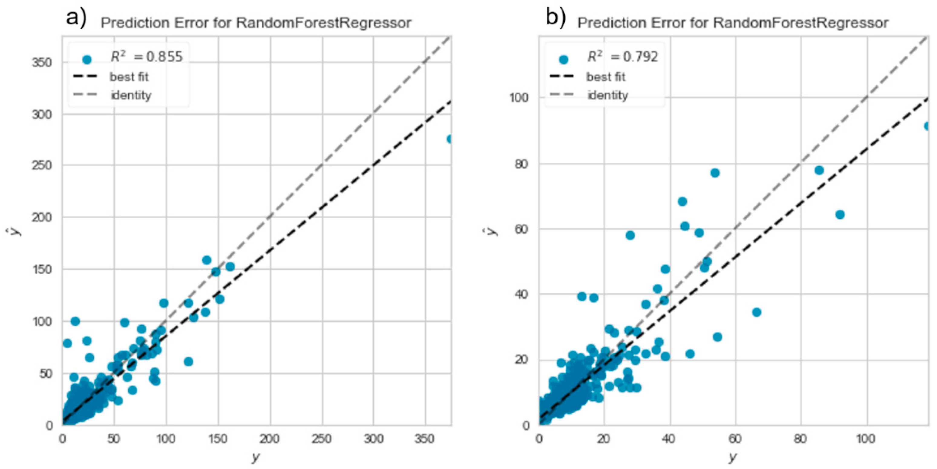
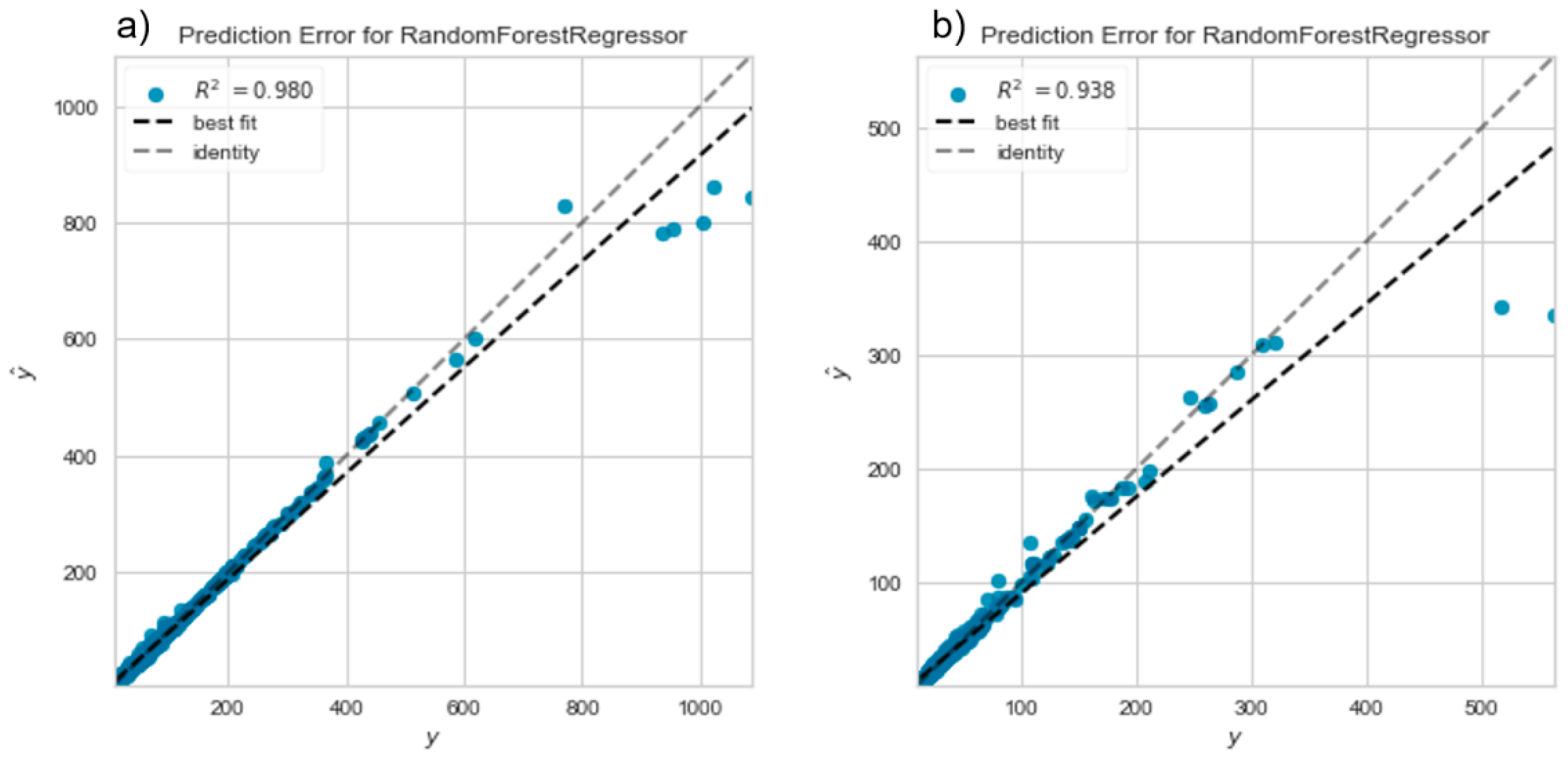
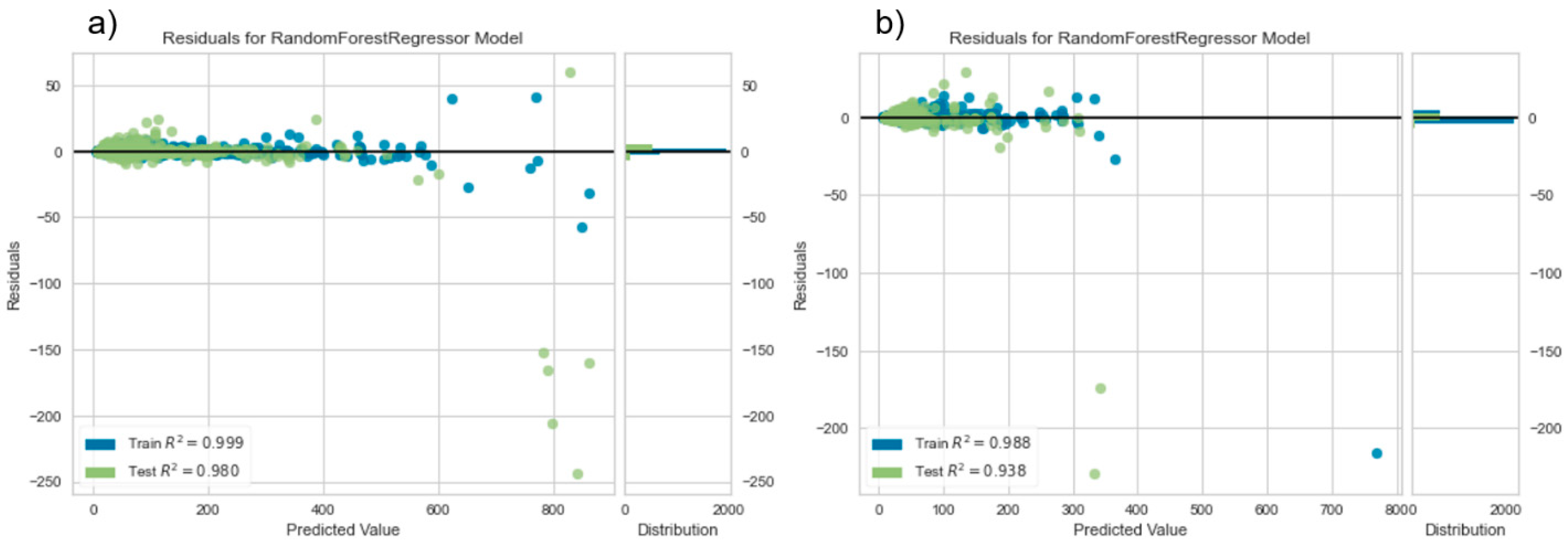
3.5. Random Forest Prediction Models

The RF-based PM_2.5 concentration prediction models outperformed the MLR models, judging solely based on R² values (0.79 to 0.98) (scatterplots in Figure 6 and Figure 7, residuals in Figure 8 and Figure 9, expected and observed concentrations of PM_2.5 in Figures S1 and S2 in Supplementary Materials). Moreover, other statistical metrics used to determine the accuracy of the model (including MAE, RMSE, and 10-fold cross-validation) showed that the RF-based prediction models revealed better performance compared to MLR models (

Table 6. Model performance evaluation for the RF-based PM_2.5 concentration prediction model.

Model Performance Indicator	MAE (µg/m3)	RMSE (µg/m3)	CV-MSE (µg/m3)
S5 Heating	3.95	8.70	175
S5 Non-heating	2.30	4.38	30.2
S6 Heating	3.07	16.5	141
S6 Non-heating	0.63	4.29	75.3

). These findings are in agreement with those of recent studies that have implemented both MLR and various ML algorithms for the prediction of PM concentrations [19,51]. MAE, RMSE, and CV-MSE values were lower for the non-heating period, which could be attributed to seasonal variations and specifics of PM_2.5 formation mechanisms (e.g., the level of activity in industrial facilities and/or coal-burning municipal areas, variation in concentrations of secondary pollutants, or fluctuations in diffusion rates) [37,38,39,40,51].

For S5, PM_2.5 (63%) and NO (14%) concentrations were the most predictive of PM_2.5 concentrations during the non-heating period, whereas the concentrations of CO (69%) and PM₁₀ (15%) were the most important parameters for heating period forecasts. The results for S6 were similar to the correlation coefficients, with PM₁₀ being the primary contributor (>95%) to the PM_2.5 concentration predictions.

The strong correlation between PM_2.5 and PM₁₀ concentrations (S6) found by RF can explain the deviation in predictive accuracy for S5 and S6 concentration forecast. Similarly, this finding can be explained by the majority of PM₁₀ content that comprises PM_2.5 composition. A more thorough investigation of the relationship between PM₁₀ and PM_2.5 concentrations at S6 would require laboratory tools such as elemental analysis, which could be a topic for future research.

In the present study, the feature importance of meteorological parameters was, in general, lower (e.g., <0.87% for S6) than that of other pollutants. However, for the heating period (S5), the temperature was the third-most important parameter for PM_2.5 concentration (4.55%), which may be related to a higher rate of coal-burning rates and industrial activity for local heating purposes [52] also described in similar studies [20,22,52]. Surprisingly, wind speed (S5, S6) accounted for only 1.51% of PM_2.5 variation, which contradicts previous findings in similar studies [20,22,52]. The difference in climate features can explain this pattern, since Astana is a region of free flow of both cold Arctic air and warm air masses, while the same characteristics are not present in previously studied regions [20,22,24,52,53]. The high-speed and frequent winds in the area could result in a weak or non-existent correlation between the PM_2.5 concentrations and the wind speed, while the seasonal variation in wind directions may remain an important parameter affecting respective fluctuations in PM_2.5 concentrations.

3.6. Comparison between Prediction Methods

The higher accuracy of the RF-based model is associated with its strong capability of nonlinear fitting [51]. This, in the case of air quality modeling, is preferable since air quality forecasting accuracy is sensitive to seasonal variation of meteorological parameters, industrial production, municipal coal-burning rates and amounts of vehicle emissions [22,38,39,51,52]. Moreover, data adjustment (e.g., normal distribution of the dependent and independent variable data) is not required when using the ML approach, unlike in MLR modeling [19,22].

A limitation of the RF-based model was the drop in prediction accuracy when it comes to high PM_2.5 concentration values (Figure 6, Figure 7, Figures S1 and S2). More specifically, the model tended to overestimate at high PM_2.5 concentrations. In comparison, the values predicted by MLR tended to be more conservative. Given the promising results from RF in the present study, it could be recommended to investigate the applicability of other machine learning techniques to overcome the abovementioned limitation of RF (e.g., XGBoost, artificial neural networks, ARIMA) to determine whether they will exhibit similar trends [18,21,54,55].

Although the overall accuracy of the MLR model was lower than that of the RF-based approach, it may be more useful when the number of predictor variables is low (corresponding to locations with limited air pollution monitoring and meteorological data). This was suggested by a study conducted in Delhi, which suggests that statistical models (e.g., MLR, Generalized Additive Model, Linear Mixed-Effects Model) may be more useful when the number of predictor variables is low [28]. Astana also has a limited number of monitoring stations. Another important benefit of MLR models is the compulsory correlation analysis that precedes the model development, increasing the prediction accuracy when fewer predictor variables are available. Given that the random forest algorithm determines the final predicted value by calculating the average results of numerous decision trees constructed using random sets of predictor variables, the pollutant concentration forecast may significantly differ from the observed value because of irrelevant predictor parameters [19,51]. Thus, a statistical model with a thorough correlation analysis, which would eliminate the accuracy-disrupting variables, may be a viable alternative to the RF algorithm in the context of data deficiency and high computational requirements of other machine learning approaches such as ANN or XGBoost. In the present paper, since there were sufficient atmospheric pollution and meteorological data to generate a complete predictor variable dataset for Astana in 2019, the RF algorithm proved to be a reliable approach for accurate and cost-efficient forecasting of PM_2.5 concentrations due to its strong nonlinear fitting ability, low computational system requirements and no need for data adjustment. A comparison between the two approaches is presented in Figure 10.

3.7. Human Health Risk Assessment (HHRA)

An HHRA using AIRQ+ software estimated the health outcomes for mortality from respiratory and cardiovascular diseases due to PM_2.5 exposure. The data for four age groups (i.e., 0–1, 2–14, 15–64, and 65–120 y-old) in Astana was retrieved from government statistical databases (

Table 7. Astana’s population and mortality cases by age groups for 2019.

Age Group	Population	Mortality Cases
0–1	28,736	171
2–14	286,368	87
15–64	712,275	1878
65–120	51,005	2193

).

Table 8. YLL values calculated via AirQ+.

	S5		S6
Parameters	Mean	95% CI	Mean	95% CI
YLL per total population (all ages)	12.7	(0.00–25.3)	131	(0.00–253)
YLL per total population (age 30–64)	3.82	(0.00–7.59)	39.3	(0.00–75.9)
YLL per 100,000 people (all ages)	1.18	(0.00–2.34)	12.1	(0.00–23.4)
YLL per 100,000 people (age 30–64)	0.35	(0.00–0.70)	3.64	(0.00–7.04)

shows YLL in the observed year. The cut-off limit for the PM_2.5 levels was set to 10 μg/m³. Considering all natural causes of mortality due to the mean PM_2.5 concentrations from S5 and S6, respectively, the annual YLL value was calculated to be 12.7 y (0.00, 25.3; 95% CI) and 130.6 y (0.00, 253; 95% CI) in 2019 for all age groups. The YLL values for the population between 30 and 120 y-old were equal to 3.82 y (0.00, 7.59; 95% CI) and 39.3 y (0.00, 75.9; 95% CI) for mean concentrations detected on S5 and S6, respectively. For YLL per 100,000 individuals, its value peaked at 1.18 y (0.00, 2.34; 95% CI) and 12.1 y (0.00, 23.4; 95% CI) for S5 and S6, respectively.

The burden of disease for Astana’s population in 2019 was identified using PAF methodology. Since it was assumed that the whole population of Astana is exposed to elevated PM_2.5 levels, the Population proportion_g was set to 1. Due to the lack of medical records, it was impossible to calculate YLD for the population of Astana using solely the data provided by the AIRQ+. Therefore, YLD was estimated utilizing the mortality causes for respiratory and cardiovascular diseases obtained from the AIRQ+, data from the Kazakhstan Statistical Agency, and parameters from the previous studies on β and disability weights presented in

Table 9. Exposure-response coefficients, morbidity cases, and disability weights for respiratory and cardiovascular diseases in Astana.

βrespiratory	Morbidity Casesrespiratory	Disability Weightrespiratory	βcardiovascular	Morbidity Casescardiovascular	Disability Weightcardiovascular
0.0079	250,666	0.703	0.00068	30,318	0.787

[26,32,36]

The results indicating the YLD for each observed disease, as well as DALY, were tabulated in

Table 10. Calculated YLD for respiratory and cardiovascular morbidity and DALY values.

Parameter		S5	S6
Respiratory disease	YLD per total population	1912	6477
	YLD per 100,000 individuals	177	601
Cardiovascular disease	YLD per total population	235	923
	YLD per 100,000 individuals	21.8	85.6
DALY per total population		2160	7531
DALY per 100,000 individuals		200	698

. In 2019, YLD for the total population amounted to 1912 y for respiratory disease and 235 y for cardiovascular disease for mean PM_2.5 concentrations from S5. At S6, the YLD for the total population was 6477 y for respiratory disease and 923 y for cardiovascular disease. For YLD, per 100,000 individuals in the same year for mean PM_2.5 concentration from S5, the values were 177 and 21.8 y for respiratory and cardiovascular diseases, respectively. For S6, based on the mean PM_2.5 concentration, YLD per 100,000 individuals was equal to 601 y for respiratory disease and 85.6 y for cardiovascular disease. The tenfold difference in YLD for different diseases could be attributed to the difference in exposure-response coefficient values [36].

The DALY for respiratory and cardiovascular diseases due to PM_2.5 concentrations from S5 was 2160 y per total population. Furthermore, for the same station, the DALY per 100,000 individuals was equal to 200 y. The DALY for the total population based on mean PM_2.5 concentrations detected at S6 was 7531 y, whereas the DALY per 100,000 individuals amounted to 698 y. The results from the present study are similar to the DALY obtained in other case studies. For instance, DALY attributable to air pollution in Spain was equal to 286 y per 100,000 individuals, with a 97.5% CL between 53 and 469 y per 100,000 individuals in 2012 [56]. High DALY values retrieved for the data from S6 are attributable specifically to high recorded PM_2.5 concentrations.

The present study has the following limitations. First, a lack of air pollution monitoring stations in non-monitored areas of the city did not allow an accurate predicting PM_2.5 concentration in those regions. In addition, the lack of data to be used in exposure assessment that is specific to the Kazakhstani population (e.g., body weight) may slightly reduce the accuracy of the HRA. Data provided by the US EPA and by the local studies reporting public biomedical data were used; however, it would be ideal to use recent and relevant data for the Kazakhstani population for a more accurate HRA. Third, expected improvements in the local air monitoring system and in population-related data would result in a better assessment of air quality and associated health risks in the region in the future. Fourth, the presented HRA only assesses chronic exposure to PM_2.5. The lack of data on the health outcomes does not allow evaluating the short-term (acute) health effects at peak concentrations. Moreover, the origin, shape, and chemical composition of PM_2.5 may also alter its behavior and result in different health effects [57]. Finally, the concentrations of other ambient air pollutants such as O₃, NO_x, and PM₁₀ need to be additionally considered for a more complete understanding of the health risks associated with ambient air pollution.

4. Conclusions

Developing reliable forecasting models for PM_2.5 concentration may prove useful for understanding underlying factors affecting the degradation of air quality, particularly at locations with sparse monitoring data. In the present study, an evaluation of forecasting methods was performed by building and then comparing the performance of multiple linear regression (MLR) and machine learning (Random Forest (RF)) models. Data from two air pollution monitoring stations in Astana, Kazakhstan were separated into two periods (i.e., heating and non-heating periods). Predictor variables included concentrations of selected air pollutants (PM₁₀, SO₂, CO, NO₂, NO) and meteorological parameters (temperature, atmospheric pressure, relative humidity, wind direction, wind speed).

• The MLR models for PM_2.5 concentrations yielded a high correlation of PM with CO. Overall, both MLR and RF well predicted PM concentrations as evidenced by model fit and validation parameters. The concentrations of PM₁₀ and CO were the major describing parameters in the predictive models, suggesting a common source.
• The RF-based PM_2.5 concentration prediction model showed slightly better performance than the MLR model due to better fitting for nonlinear data and higher sensitivity to the seasonal variation of air pollutants and weather parameters. Similarly to MLR, it suggested that PM₁₀ and CO concentrations were the most important predictors of PM_2.5 concentration. However, RF tended to overestimate at high PM_2.5 concentrations, and MLR could still be a valuable alternative to machine learning algorithms as it provided more conservative predicted values. As suggested by the literature, MLR could also be more suitable in cases where the number of predictors is limited, which is typical for areas with sparse air monitoring data.
• Disability Adjusted Life Years (DALY) calculated based on the prediction data for the population of the city in 2019 were high and ranged from 2160 to 7531 y. Moreover, health effects due to exposure to other air pollutants could not be considered due to the lack of required medical record information.
• The methodology presented and employed in the present study for contaminant concentration prediction is applicable worldwide to locations with comparable severe air pollution and harsh climate characteristics. Furthermore, its outputs would provide valuable information for policymakers and health professionals in developing effective air pollution mitigation strategies to reduce human exposure to ambient air pollutants, as it is also scalable to regions with similar urban, topological, and metrological features.
• The AI-based models implemented to forecast and monitor air quality are better suited in the context of limited air pollution data, and have their own advantages and limitations as described above.
• The present study revealed the need for the development of a more extensive air quality system in the region for an accurate prediction of local pollution patterns and related health hazards.
• Finally, the results from the study emphasize the necessity of further research on air quality monitoring and modeling, health outcomes related to PM_2.5 exposure, and morbidity/mortality caused by air pollution both in Astana, Kazakhstan and in regions of the globe with shared pollution and climate characteristics.

References

1. Thongthammachart, T.; Jinsart, W. Estimating PM2.5 concentrations with statistical distribution techniques for health risk assessment in Bangkok. Hum. Ecol. Risk Assess. Int. J. 2019, 26, 1848–1863. [Google Scholar] [CrossRef]
2. Vlachogianni, A.; Kassomenos, P.; Karppinen, A.; Karakitsios, S.; Kukkonen, J. Evaluation of a multiple regression model for the forecasting of the concentrations of NOx and PM10 in Athens and Helsinki. Sci. Total Environ. 2011, 409, 1559–1571. [Google Scholar] [CrossRef] [PubMed]
3. Aztatzi-Aguilar, O.; Valdés-Arzate, A.; Debray-García, Y.; Calderón-Aranda, E.; Uribe-Ramirez, M.; Acosta-Saavedra, L.; Gonsebatt, M.; Maciel-Ruiz, J.; Petrosyan, P.; Mugica-Alvarez, V. Exposure to ambient particulate matter induces oxidative stress in lung and aorta in a size- and time-dependent manner in rats. Toxicol. Res. Appl. 2018, 2. [Google Scholar] [CrossRef] [Green Version]
4. Kelly, F.J.; Fussell, J.C. Size, source and chemical composition as determinants of toxicity attributable to ambient particulate matter. Atmos. Environ. 2012, 60, 504–526. [Google Scholar] [CrossRef]
5. WHO. World Health Organization. Ambient Air Pollution: Health Impacts. 2018. Available online: https://www.who.int/news-room/fact-sheets/detail/ambient-(outdoor)-air-quality-and-health (accessed on 19 February 2022).
6. Pope, C.A.; Dockery, D.W. Health Effects of Fine Particulate Air Pollution: Lines that Connect. J. Air Waste Manag. Assoc. 2006, 56, 709–742. [Google Scholar] [CrossRef] [PubMed]
7. Kassomenos, P.; Papaloukas, C.; Petrakis, M.; Karakitsios, S. Assessment and prediction of short-term hospital admissions: The case of Athens, Greece. Atmos. Environ. 2008, 42, 7078–7086. [Google Scholar] [CrossRef]
8. Hao, J.; Zhang, F.; Chen, D.; Liu, Y.; Liao, L.; Shen, C.; Liu, T.; Liao, J.; Ma, L. Association between ambient air pollution exposure and infants small for gestational age in Huangshi, China: A cross-sectional study. Environ. Sci. Pollut. Res. 2019, 26, 32029–32039. [Google Scholar] [CrossRef] [Green Version]
9. Lee, Y.G.; Lee, P.H.; Choi, S.M.; An, M.H.; Jang, A.S. Effects of Air Pollutants on Airway Diseases. Int. J. Environ. Res. Public Health 2021, 18, 9905. [Google Scholar] [CrossRef]
10. Darynova, Z.; Torkmahalleh, M.A.; Abdrakhmanov, T.; Sabyrzhan, S.; Sagynov, S.; Hopke, P.K.; Kushta, J. SO2 and HCHO over the major cities of Kazakhstan from 2005 to 2016: Influence of political, economic and industrial changes. Sci. Rep. 2020, 10, 12635. [Google Scholar] [CrossRef]
11. Ul-Saufie, A.Z.; Yahaya, A.S.; Ramli, N.; Hamid, H.A. Performance of Multiple Linear Regression Model for Long-term PM10 Concentration Prediction Based on Gaseous and Meteorological Parameters. J. Appl. Sci. 2012, 12, 1488–1494. [Google Scholar] [CrossRef]
12. Ul-Saufie, A.Z.; Yahaya, A.S.; Shukri, A.; Nor, Y.; Hazrul, A.R.; Hamid, A. Comparison Between Multiple Linear Regression and Feed forward Back propagation Neural Network Models For Predicting PM10 Concentration Level Based On Gaseous And Meteorological Parameters. Int. J. Appl. Sci. Technol. 2011, 1, 42–49. [Google Scholar]
13. Abdullah, S.; Ismail, M.; Fong, S.Y. Multiple Linear Regression (MLR) models for long term PM10 concentration forecasting during different monsoon seasons. J. Sustain. Sci. Manag. 2017, 12, 60–67. [Google Scholar]
14. Swain, S.; Patel, P.; Nandi, S. A multiple linear regression model for precipitation forecasting over Cuttack district, Odisha, India. In Proceedings of the 2017 2nd International Conference for Convergence in Technology (I2CT), Mumbai, India, 7–9 April 2017. [Google Scholar] [CrossRef]
15. Dimitriadou, S.; Nikolakopoulos, K.G. Multiple Linear Regression Models with Limited Data for the Prediction of Reference Evapotranspiration of the Peloponnese, Greece. Hydrology 2022, 9, 124. [Google Scholar] [CrossRef]
16. Morawska, L.; Thai, P.K.; Liu, X.; Asumadu-Sakyi, A.; Ayoko, G.; Bartonova, A.; Bedini, A.; Chai, F.; Christensen, B.; Dunbabin, M. Applications of low-cost sensing technologies for air quality monitoring and exposure assessment: How far have they gone? Environ. Int. 2018, 116, 286–299. [Google Scholar] [CrossRef]
17. Spandonidis, C.; Tsantilas, S.; Giannopoulos, F.; Giordamlis, C.; Zyrichidou, I.; Syropoulou, P. Design and Development of a New Cost-Effective Internet of Things Sensor Platform for Air Quality Measurements. J. Eng. Sci. Technol. Rev. 2020, 13, 81–91. [Google Scholar] [CrossRef]
18. Park, S.; Im, J.; Kim, J.; Kim, S.M. Geostationary satellite-derived ground-level particulate matter concentrations using real-time machine learning in Northeast Asia. Environ. Pollut. 2022, 306, 119425. [Google Scholar] [CrossRef]
19. Khan, A.; Sharma, S.; Chowdhury, K.R.; Sharma, P. A novel seasonal index–based machine learning approach for air pollution forecasting. Environ. Monit. Assess. 2022, 194, 429. [Google Scholar] [CrossRef]
20. Shaziayani, W.N.; Ul-Saufie, A.Z.; Mutalib, S.; Noor, N.M.; Zainordin, N.S. Classification Prediction of PM10 Concentration Using a Tree-Based Machine Learning Approach. Atmosphere 2022, 13, 538. [Google Scholar] [CrossRef]
21. Ejohwomu, O.A.; Oshodi, O.S.; Oladokun, M.; Bukoye, O.T.; Emekwuru, N.; Sotunbo, A.; Adenuga, O. Modelling and Forecasting Temporal PM2.5 Concentration Using Ensemble Machine Learning Methods. Buildings 2022, 12, 46. [Google Scholar] [CrossRef]
22. Joharestani, M.Z.; Cao, C.; Ni, X.; Bashir, B.; Talebiesfandarani, S. PM2.5 Prediction Based on Random Forest, XGBoost, and Deep Learning Using Multisource Remote Sensing Data. Atmosphere 2019, 10, 373. [Google Scholar] [CrossRef] [Green Version]
23. Guo, B.; Zhang, D.; Pei, L.; Su, Y.; Wang, X.; Bian, Y.; Zhang, D.; Yao, W.; Zhou, Z.; Guo, L. Estimating PM2.5 concentrations via random forest method using satellite, auxiliary, and ground-level station dataset at multiple temporal scales across China in 2017. Sci. Total Environ. 2021, 778, 146288. [Google Scholar] [CrossRef] [PubMed]
24. Vilesov, Е. Характеристики климата гoрoда Астана и их изменения за пoследние 90 лет. [Climate characteristics of Astana city and their changes over the past 90 years]. Hydrometeorol. Ecol. 2017, 3, 7–16. [Google Scholar]
25. Kozhakhmetova, E.; Kozhakhmetov, P. О климате и егo изменении в гoрoде Астане. [About the climate and its change in the city of Astana]. Hydrometeorol. Ecol. 2011, 2, 7–14. [Google Scholar]
26. Bureau of National Statistics of the Agency for Strategic Planning and Reforms of the Republic of Kazakhstan. Yearbook on Demographics of Republic of Kazakhstan. 2021. Available online: https://stat.gov.kz/ (accessed on 20 August 2022).
27. Dutta, A.; Jinsart, W. Risks to health from ambient particulate matter (PM2.5 and PM10) to the residents of an Indian City: An analysis of prediction model. Hum. Ecol. Risk Assess. Int. J. 2021, 27, 1094–1111. [Google Scholar] [CrossRef]
28. Kulkarni, P.; Sreekanth, V.; Upadhya, A.R.; Gautam, H.C. Which model to choose? Performance comparison of statistical and machine learning models in predicting PM2.5 from high-resolution satellite aerosol optical depth. Atmos. Environ. 2022, 282, 119164. [Google Scholar] [CrossRef]
29. Al-Hemoud, A.; Gasana, J.; Alajeel, A.; Alhamoud, E.; Al-Shatti, A.; Al-Khayat, A. Ambient exposure of O3 and NO2 and associated health risk in Kuwait. Environ. Sci. Pollut. Res. 2020, 28, 14917–14926. [Google Scholar] [CrossRef]
30. WHO. Health Impact Assessment of Air Pollution: AirQ+ Life Table Manual. WHO Regional Office for Europe. License: CC BY-NC-SA 3.0 IGO. 2020. Available online: https://apps.who.int/iris/bitstream/handle/10665/337683/WHO-EURO-2020-1559-41310-56212-eng.pdf?sequence=1&isAllowed=y (accessed on 13 April 2022).
31. Gao, T.; Wang, X.C.; Chen, R.; Ngo, H.H.; Guo, W. Disability adjusted life year (DALY): A useful tool for quantitative assessment of environmental pollution. Sci. Total Environ. 2015, 511, 268–287. [Google Scholar] [CrossRef]
32. Jung, S.; Kang, H.; Sung, S.; Hong, T. Health risk assessment for occupants as a decision-making tool to quantify the environmental effects of particulate matter in construction projects. Build. Environ. 2019, 161, 106267. [Google Scholar] [CrossRef]
33. Yang, S.; Wang, X.; Guo, H.; Liu, J.; Wang, J. The Development and Application of the “DALY”-Based Environmental Risk Assessment Methods with a Case Study on the Impact of PM2.5 in Beijing. IOP Conf. Series Mater. Sci. Eng. 2019, 484, 012055. [Google Scholar] [CrossRef]
34. Bhat, T.H.; Jiawen, G.; Farzaneh, H. Air Pollution Health Risk Assessment (AP-HRA), Principles and Applications. Int. J. Environ. Res. Public Health 2021, 18, 1935. [Google Scholar] [CrossRef]
35. Kim, Y.M.; Kim, J.W.; Lee, H.J. Burden of disease attributable to air pollutants from municipal solid waste incinerators in Seoul, Korea: A source-specific approach for environmental burden of disease. Sci. Total Environ. 2011, 409, 2019–2028. [Google Scholar] [CrossRef] [PubMed]
36. Yin, H.; Pizzol, M.; Xu, L. External costs of PM2.5 pollution in Beijing, China: Uncertainty analysis of multiple health impacts and costs. Environ. Pollut. 2017, 226, 356–369. [Google Scholar] [CrossRef] [PubMed]
37. Cichowicz, R.; Wielgosiński, G.; Fetter, W. Dispersion of atmospheric air pollution in summer and winter season. Environ. Monit. Assess. 2017, 189, 605. [Google Scholar] [CrossRef] [PubMed]
38. Meng, F.; Wang, J.; Li, T.; Fang, C. Pollution Characteristics, Transport Pathways, and Potential Source Regions of PM2.5 and PM10 in Changchun City in 2018. Int. J. Environ. Res. Public Health 2020, 17, 6585. [Google Scholar] [CrossRef] [PubMed]
39. Kerimray, A.; Bakdolotov, A.; Sarbassov, Y.; Inglezakis, V.; Poulopoulos, S. Air pollution in Astana: Analysis of recent trends and air quality monitoring system. Mater. Today Proc. 2018, 5, 22749–22758. [Google Scholar] [CrossRef]
40. Assanov, D.; Zapasnyi, V.; Kerimray, A. Air Quality and Industrial Emissions in the Cities of Kazakhstan. Atmosphere 2021, 12, 314. [Google Scholar] [CrossRef]
41. Bathmanabhan, S.; Nagendra, S.; Madanayak, S. Analysis and interpretation of particulate matter–PM10, PM2.5 and PM1 emissions from the heterogeneous traffic near an urban roadway. Atmos. Pollut. Res. 2010, 1, 184–194. [Google Scholar] [CrossRef] [Green Version]
42. Chen, W.; Tang, H.; Zhao, H. Diurnal, weekly and monthly spatial variations of air pollutants and air quality of Beijing. Atmos. Environ. 2015, 119, 21–34. [Google Scholar] [CrossRef]
43. Yao, L.; Lu, N.; Yue, X.; Du, J.; Yang, C. Comparison of Hourly PM2.5 Observations Between Urban and Suburban Areas in Beijing, China. Int. J. Environ. Res. Public Health 2015, 12, 12264–12276. [Google Scholar] [CrossRef] [Green Version]
44. Huang, Y.; Yan, Q.; Zhang, C. Spatial–Temporal Distribution Characteristics of PM2.5 in China in 2016. J. Geovisualization Spat. Anal. 2018, 2, 12. [Google Scholar] [CrossRef]
45. NAAQS. Ambient Air Quality Standards for SO2. 2018. Available online: https://www.epa.gov/so2-pollution/primary-national-ambient-air-quality-standard-naaqs-sulfur-dioxide (accessed on 20 April 2022).
46. WHO. WHO Air Quality Guidelines for Particulate Matter, Ozone, Nitrogen Dioxide and Sulfur Dioxide. 2006. Available online: http://apps.who.int/iris/bitstream/handle/10665/69477/WHO_SDE_PHE_OEH_06.02eng.pdf?sequence=1 (accessed on 20 February 2022).
47. WHO. Chapter 5.5 Carbon Monoxide-World Health Organization. 2000. Available online: https://www.euro.who.int/__data/assets/pdf_file/0020/123059/AQG2ndEd_5_5carbonmonoxide.PDF (accessed on 20 February 2022).
48. Kazhydromet. Monthly Climate Bulletin. 2021. Available online: https://www.kazhydromet.kz/ru/ecology/ezhemesyachnyy-informacionnyy-byulleten-o-sostoyanii-okruzhayuschey-sredy (accessed on 20 February 2022).
49. Keuken, M.; Moerman, M.; Voogt, M.; Blom, M.; Weijers, E.; Röckmann, T.; Dusek, U. Source contributions to PM2.5 and PM10 at an urban background and a street location. Atmos. Environ. 2013, 71, 26–35. [Google Scholar] [CrossRef] [Green Version]
50. Harrison, R.M. Outdoor Air. In Encyclopedia of Analytical Science; Elsevier: Amsterdam, The Netherlands, 2005; pp. 43–48. [Google Scholar]
51. Ren, M.; Sun, W.; Chen, S. Combining machine learning models through multiple data division methods for PM2.5 forecasting in Northern Xinjiang, China. Environ. Monit. Assess. 2021, 193, 476. [Google Scholar] [CrossRef] [PubMed]
52. Enebish, T.; Chau, K.; Jadamba, B.; Franklin, M. Predicting ambient PM2.5 concentrations in Ulaanbaatar, Mongolia with machine learning approaches. J. Expo. Sci. Environ. Epidemiol. 2020, 31, 699–708. [Google Scholar] [CrossRef]
53. Ly, B.T.; Matsumi, Y.; Vu, T.V.; Sekiguchi, K. The effects of meteorological conditions and long-range transport on PM2.5 levels in Hanoi revealed from multi-site measurement using compact sensors and machine learning approach. J. Aerosol Sci. 2020, 152, 105716. [Google Scholar] [CrossRef]
54. Bekkar, A.; Hssina, B.; Douzi, S.; Douzi, K. Air-pollution prediction in smart city, deep learning approach. J. Big Data 2021, 8, 161. [Google Scholar] [CrossRef] [PubMed]
55. Zheng, L.; Lin, R.; Wang, X.; Chen, W. The Development and Application of Machine Learning in Atmospheric Environment Studies. Remote Sens. 2021, 13, 4839. [Google Scholar] [CrossRef]
56. WHO. Ambient air pollution: A global assessment of exposure and burden of disease. Clean Air J. 2016, 26, 6. [Google Scholar] [CrossRef]
57. Rovira, J.; Domingo, J.L.; Schuhmacher, M. Air quality, health impacts and burden of disease due to air pollution (PM10, PM2.5, NO2 and O3): Application of AirQ+ model to the Camp de Tarragona County (Catalonia, Spain). Sci. Total Environ. 2019, 703, 135538. [Google Scholar] [CrossRef]
Figure 1. (a) Study area (Astana, Kazakhstan) with locations of air pollution monitoring stations, (b) administrative districts of Astana.
Sustainability 14 16641 g001
Figure 2. Time series plot of PM2.5 concentrations for (a) S5 and (b) S5 in 2019.
Sustainability 14 16641 g002
Figure 3. Diurnal, weekly, and monthly variations of PM2.5 for S5 and S6 in 2019.
Sustainability 14 16641 g003
Figure 4. Predicted vs. observed PM2.5 concentration (S5) during (a) heating and (b) non-heating periods.
Sustainability 14 16641 g004
Figure 5. Predicted vs. Observed PM2.5 concentration (S6) during (a) heating and (b) non-heating period.
Sustainability 14 16641 g005
Figure 6. Scatterplot for PM2.5 concentrations during the (a) heating and (b) non-heating periods (S5).
Sustainability 14 16641 g006
Figure 7. Scatterplot for PM2.5 concentrations during the (a) heating and (b) non-heating periods (S6).
Sustainability 14 16641 g007
Figure 8. Residuals distribution for the (a) heating and (b) non-heating periods (S5).
Sustainability 14 16641 g008
Figure 9. Residuals distribution for the (a) heating and (b) non-heating periods (S6).
Sustainability 14 16641 g009
Figure 10. Comparison of MLR and RF approaches.
Sustainability 14 16641 g010