Abstract
The primary objective of this research is to assess the hydrogeochemical features and water quality of the Thamirabarani river stretch, located in southern India. Thirty-five water samples from the Thamirabarani river stretch were obtained from the districts of Tirunelveli and Thoothukudi. Twelve water quality parameters were measured during the pre-monsoon and post-monsoon periods of 2020 and 2021. The analytical results were verified with BIS and WHO standards to evaluate the water for drinking purposes. A Geographic Information system (GIS) was applied to know the spatial variation of the hydrogeochemical properties over the research area. Moreover, the Water Quality Index was calculated and it was revealed that 15% of the water samples used are outstanding, 35% are fit for potable use, 25% are poor, 15% water are very poor, and 10% unfit for consumption. Principal Component analysis (PCA) was performed to find out the dominant factors and their variance coverage for the overall water quality. The PCA results indicate that a water sample in Zone 1 is known for its alkalinity. The water qualities in Zone 2 and Zone 3 were affected by anthropogenic factors and industry wastes. More sea water intrusion was observed in Zone 4 in the water quality of the Thamirabarani river basin.
1. Introduction
Human civilization, living species, and natural habitats all require water. Water is nature’s elixir of life, a priceless gift to humans and millions of other animals. Rivers are one of the world’s most vital resources of water. Rivers and streams have long been a vital part of the hydrological cycle, helping to maintain the world’s continual flow of water [1]. Rivers can offer freshwater for domestic consumption, livelihood, and commercial production (agricultural, cattle, and fisheries), as well as navigation and tourism [2]. River ecosystems also play a significant role in environmental regulation, transporting nutrients, assimilation of municipal and industrial waste, and flood and drought control. Many of these functions are inextricably linked to river health indicators such as water quality, ecological state, and flow.
Rapid industrialization to support the nation’s economy and growing population has affected the health of rivers around the world. The majority of rivers that go through cities receive municipal trash and industrial effluents [1]. Phenols, suspended particles, pesticides, oils, plastics, grease, heavy metals, plasticizers, and solvents are among the organic as well as inorganic contaminants found in wastewater from industry and agricultural runoffs [3]. The continuous discharge of urban wastewater, industrial effluents, and seasonal surface run-off as a result of climate change has an impact not just on water quality but also on river discharge [4,5]. Still, rivers are the primary water sources for many reasons in an area, including agricultural, human consumption, and industrial needs [6]. One of the most significant challenges affecting human health is the deterioration of the quality of river water [7]. River water pollution has a negative impact not just on humans, but also on aquatic flora and animals, putting their survival at risk.
Water quality testing is important for assessing the ecosystem’s health and for facilitating the appropriate management procedures required to safeguard water resources from pollution sources. The discipline of environmental research that uses multivariate statistical models is known as environmetrics or chemometrics [8]. Multivariate statistical techniques can expose hidden data in huge amounts of water quality data and prevent the data from being misinterpreted by the monitoring system. They are critical in validating temporal as well as spatial fluctuations induced by natural and manmade processes, assisting in locating the latent pollution sources.
Multivariate analysis entails evaluating more than two water quality factors at the same time [9]. Multivariate analysis refers to any statistical approach that deals with the instantaneous analysis of different measurements across multiple factors. These data mining approaches are particularly useful for pattern detection and data exploration, which extract hidden data from a database [10]. Principal Component Analysis (PCA), Factor analysis, Cluster Analysis (CA), discriminant analysis, and multiple linear regression are some of the most often used multivariate statistical models for analyzing and interpreting environmental data [11].
Water quality regulations and monitoring programs generate a vast number of multidimensional water quality parameter sets, pollution characteristics, and numerical data about various water sources that are understandable to scientists. This information, however, should be beneficial to water sector managers in making decisions who want to update the condition of their water sources [12]. As a result, a technique known as the Water Quality Index was developed to solve this issue. The Water Quality Index is a quantitative representation that is used to determine the ecological health of a body of water [13,14,15]. The purpose of the Water Quality Index is to categorize waters according to their physical, chemical, and biological attributes, thereby establishing their potential uses and controlling their allocation decisions [16]. By providing a single dimensionless value, the WQI hopes to reduce the multivariate nature of the data that describes the quality of water [17,18]. A single WQI number is easier to understand and remember than a big list of statistical data revealing a wide range of characteristics. WQIs also allow for comparisons across different sample locations and events. As a result, they are thought to be more effective at disseminating information to general audiences and decision-makers for effective water resource management [19].
The motivation for this study is to gain clarity on the water quality of the Thamirabarani river stretch and how it varies when it flows through different districts. This water quality assessment study employs novel approaches by analyzing the causes of water quality deterioration. This study can serve as a good model for the district authorities and decision makers to consider the various factors that lead to water quality variation from the headwaters to the estuary.
2. Materials and Methods
2.1. Study Area
The Thamirabarani river is amongst the most valuable perennial rivers in Tamilnadu, flowing through Tirunelveli and Thoothukudi. It is a reliable water source for irrigation, drinking, and electricity generation [20]. Numerous reservoirs, aqueducts, and dams on the Thamirabarani River supply a substantial amount of water for irrigation and as a power source in the Tirunelveli district. This river is the only source of drinking water for the entire district and paddy cultivation is the main agricultural activity carried out here [21].
This basin’s irrigation system is centuries old and well established, complete with its own ayacut system. It flows first northeast at first, then east in the middle, and finally confluences with the Bay of Bengal near PazhayaKaayal.
The southwest and northeast monsoons have an impact on the climatic conditions in this basin. Thamirabarani means “carrier of copper” in Tamil, since the river sand contains copper.
The Thamirabarani River Basin covers the districts of Tirunelveli and Thoothukudi and is 1 of 17 river basins with seven sub-basins. The Thamirabarani River Basin is located between geographic coordinates N. lat. 8°26′45″ to 9°12′00″ and E. long. 77°09′00″ to 78°08′30″. The river flows through many Taluks of Tirunelveli as well as the Thoothukudi districts of Tamilnadu [22].
The total study area is divided into 4 Zones for this research so that it provides much clarity and deeper insights into the sampling sights. The objective of this study is to analyze the water samples from all three courses of the river. Thus, these 35 samples represent the full main course of the Thamirabarani river basin. Each taluk is considered as a zone in this research work. Zone 2 contains both the Taluks Tirunelveli and Palayamkottai. Since both are twin cities, they are close to each other and share many locations, so they are clubbed together to form a single zone. The government of Tamilnadu separated these as two different Taluks just for administration purposes.
The study areas along with the sampling sites are provided in Figure 1.
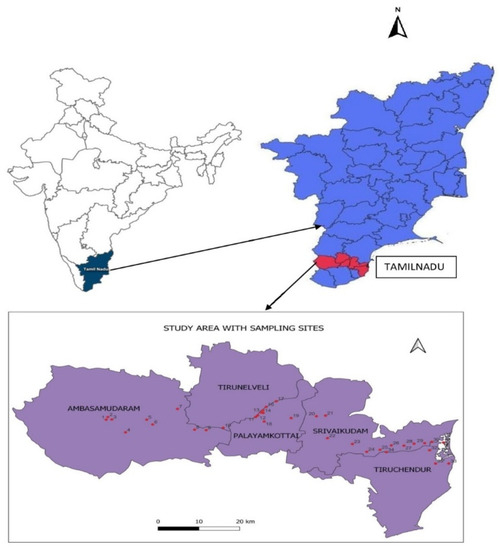
Figure 1.
Study area. Taluks of Tirunelveli and Thamirabarani with sampling points. (Source—ArcGIS).
The Zones classified are as below:
- Zone 1 consists of the Ambasamudram Taluk.
- This zone covers the upper course of the river. This taluk has the Agasthiar Falls sampling point, which is the source point of the Thamirabarani river.
- Zone 2 consists of the Tirunelveli and Palayamkottai taluks combined together.
- This zone covers the middle course of the river. This is the most urbanized zone in this study. Tirunelveli is an ancient city and an important corporation in southern Tamilnadu.
- Zone 3 consists of Srivaikundam Taluk.
- This zone covers the stations, which are mainly in the Thoothukudi district.
- Zone 4 consists of Tiruchendur Taluk.
- This zone covers the lower course of the river. This zone contains most of the coastal areas.
2.2. Sample Collection
The water samples were collected in 2-L HDPE bottles for physicochemical analysis according to standard protocols [23]. To remove the impurities, all sampling bottles were cleaned and acid washed in the laboratory using 10% hydrochloric acid (HCl). The bottles were cleaned twice more with the sample water at the sampling location before being labeled. The water samples were collected at 35 sites from Agasthiar falls to the Punnaikayal coastal region along the stretch of Thamirabarani river basin.
The water’s quality was determined by comparing each metric to the standard desired limit set forth in BIS 10500: 2012. The parameters tested are pH, Bicarbonate (HCO3), Sulphate (SO4), Sodium (Na), Total Dissolved Solid (TDS), Chloride (Cl), Nitrate (NO3), Calcium (Ca), Fluoride (F), Potassium (K), and Magnesium (Mg). The statistical analyses were carried out with these observed parameters. Table 1 shows the list of sample collection sites along with their geographic location.

Table 1.
Sample collection sites and their geographic location.
2.3. Field and Laboratory Setup
The water was collected from the sampling sites provided above and care was taken to ensure that the water collection was not performed in stagnant water [24,25].
After cleaning the bottles 2–3 times with the water to be analyzed, the river water samples were extracted in pre-washed 2-L HDPE narrow mouth bottles [26]. A total of 35 water samples were extracted from the Thamirabarani watershed, with each sample being collected in a grid to provide for improved spatial interpolation and coverage of the whole study region [27]. The in situ measurements of physicochemical parameters such as pH and TDS were created with a Hanna portable instrument (model HI 98130). The samples were sent to the Government Engineering College, Tirunelveli. They were analyzed in the Environmental Geochemistry Laboratory within 48 h. Standard titration was used to determine the Cl, TH, Ca, and Mg [28]. A turbidity meter was utilized to determine the SO4 content in the water samples. The ultraviolet spectrophotometric method was adopted for determining the NO3 levels in the water samples.
Table 2 shows the different methods employed to find out the physicochemical properties.
Table 2.
Methods used for physicochemical studies.
2.4. Spatial Interpolation Using GIS
GIS is an indispensable tool for natural resource management, particularly in the areas of land use planning, animal habitat analysis, and natural hazard assessment to name a few of its many applications [29]. Although statistical surfaces, in the sense that they are defined by cartographers, do not exist in the same way that land does, it is possible to conceptualize them in the same way [30,31]. For the preparation of statistical surfaces, the spatial interpolation process in GIS is commonly utilized [32]. Given the impossibility of collecting field data at every location in the study area, we had to resort to spatial interpolation methods to extrapolate information from sampled locations to locations where it could not be collected.
Aiming toward the creation of maps depicting the spatial distribution of water quality parameters, ArcInfo 10 GIS software was used to correlate the water quality and WQI data to the sampling locations [33]. There are various spatial interpolation methods available. The inverse distance weighting (IDW) method is used in this study.
Finally, using the spatial interpolation method, maps depicting the spatial distribution were created. Identifying variations in the accumulations of various parameters in the surface water of the research area was performed.
2.5. Water Quality Index
The WQI, similar to many other index systems, assigns a common scale to a group of water quality metrics before combining them into a single numerical value using the selected computation technique. The WQI is intended to be used to monitor water quality trends for management and decision-making purposes rather than as an absolute measure of contamination [34].
The WQI is an index that measures the combined influence of numerous water quality variables [35]. The water quality index was established to analyze natural and artificial activities based on fundamental groundwater chemistry markers. The water quality index can also assess the quality of water in general as well as in terms of its intended use: for drinking, for recreation, for the aquatic zone, for agriculture, etc. [36,37].
There are many water quality index calculation methods available for determining the water quality such as National Sanitation Foundation WQI, Oregon WQI, Weighted Arithmetic WQI, and Canadian Council of Ministers of the Environment WQI. In this study, the National Sanitation Foundation WQI calculation designed by Brown [17] was used since it has the following advantages.
- This method of calculation is quick, objective, and reproducible and it condenses all of the data that pertains to the analyzed parameters into a single value.
- The evaluation of changes in water quality in various regions [37].
The weights that were applied to the physico-chemical properties in order to calculate the WQI were determined based on their relative importance in terms of the overall water quality for the purposes of drinking water. The allotted weight is a number between 1 and 5. NO3 and TDS were assigned a maximum weight of 5, pH and SO4 were assigned as 4, HCO3 was assigned as 3, Cl and TH were assigned as 2, and Ca, Na, K, and Mg were assigned as 1 [38].
Then, the relative weight (Wi) was determined by using the equation below.
where Wi is the relative weight; wi is the weight of each parameter; and n is the number of parameters.
Table 3 lists the different parameters and their relative weights. In the following stage, a quality rating scale known as qi was calculated for each parameter by dividing the parameter’s concentration in each water sample by the standard associated with that concentration, as outlined in BIS 10500 (1991), and then multiplying the result by 100
where, qi is the quality rating; Ci is the concentration of each chemical parameter in each water sample in mg/L; and Si is the Indian drinking water standard for each chemical parameter in mg/L according to the guidelines of the BIS 10500.
qi = (Ci/Si) × 100
Table 3.
Parameters with their weights.
The SI for each chemical parameter is found first, which is then utilized to find the WQI using the below equation.
where SIi is the sub-index of ith parameter; qi is the rating based on the concentration of ith parameter; and n is the number of parameters.
SIi = Wi × qi
WQI = _SIi
2.6. Principal Component Analysis
2.6.1. Pretreatment
The initial data organization was performed based on the sites and year of monitoring. Any missing readings from the stations were assigned the mean value of the dataset [39]. The water quality parameters were measured on a variety of scales, each with a unique range of values. Hence, data standardization was performed in order to generate a normally distributed sample of all variables [40]. Several sets of data that do not follow a normal distribution were pretreated using a method that is a hybrid of standardization, log-scaling, and centering. Then, this data output is fed into the Principal Component analyzing tool.
2.6.2. Analysis
Multivariate analysis of the water samples was conducted using Principal Component Analysis. PCA is also utilized to reduce the huge amount of data into some meaningful, simpler data that can be further used to find out the prominent factors that are responsible for the variation of the water quality characteristics [41]. To achieve this, MS Excel 2016 and IBM SPSS Statistics 28.0.0.0 (Armonk, NY, USA) were used. SPSS (Statistical Package for the Social Sciences) is a software tool that is frequently utilized frequently for the purpose of statistical analysis in a variety of fields. It has numerous applications in dealing with data. IBM SPSS is well-known for its applications, which include advanced statistical analysis, pre-processing, processing, and analysis of data [42]. IBM SPSS is used in different fields such as stock market research, survey marketing, government organizations, information technology, etc. The normalization and dimension reduction methods of SPSS were utilized in this study. The input data were fed to the Dimension reduction menu in SPSS for generating principal components. PCA was conducted on the variables that had been normalized in order to obtain major principal components (PCs) and also to minimize the participation of variables that had a minor significance. These PCs were then exposed to varimax rotation (raw) in order to generate Varifactors using Varimax with a Kaiser normalization method.
3. Results
3.1. Hydrogeochemistry
The quality of river water is determined by a complicated web of interactions between physical, biological, and chemical factors [43]. Water quality monitoring of rivers in the country have received a lot of attention, with the goal of determining the causes of their deterioration and identifying the most contaminated river segments in the country.
The zone-wise average values of the chemical parameters are provided in Figure 2.
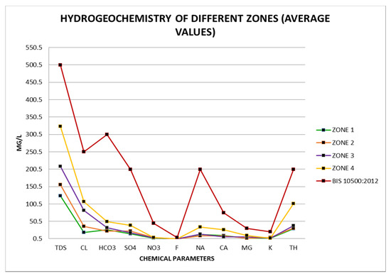
Figure 2.
An overview of the chemical parameters (Zone-wise average).
The pH value of natural water is determined by the interaction of several factors, such as the equilibrium of carbon dioxide, carbonate, and HCO3 [44]. The pH of the water is the most essential and decisive element in determining the corrosivity of water. Under Zone 1, the pH values were observed between 6.14 and 8.7. Few stations such as V.K. Puram and Cheranmahadevi have a higher range of pH that is above the desirable limit of the BIS standard, while other stations have their pH range within the standard limits. The industrial effluent discharge into this zone is observed in V.K. Puram and the urban waste disposal observed in Cheranmahadevi could be the cause of the high pH. Under Zone 2, the pH values were observed between 7.3 and 7.88, which are within the desirable limit of the BIS standard of from 6.5 to 8.5. Under Zone 3, the pH values were observed between 7 and 8.2, which is within the desirable limit of BIS standards. Under Zone 4, the pH values were observed between 6.6 and 8.48, which are within the desirable limit of the BIS standard, but still the coastal site Senthapoomangalam records the highest pH value of 8.48. The spatial distribution of PH over the entire zone is provided in Figure 3a. It is evident from this figure that the pH value is very high at the coastal sites
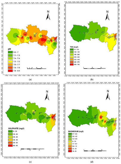
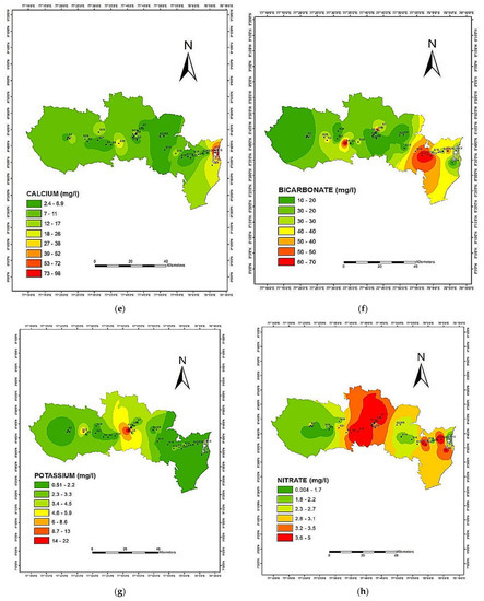
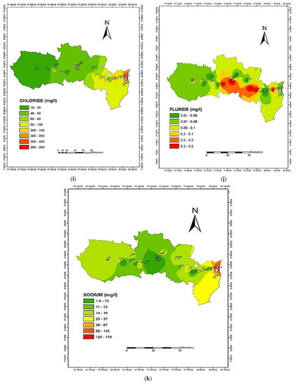
Figure 3.
(a) Spatial distribution of pH; (b) Spatial distribution of TDS; (c) Spatial distribution of SO4; (d) Spatial distribution of Mg; (e) Spatial distribution of Ca; (f) Spatial distribution of HCO3; (g) Spatial distribution of K; (h) Spatial distribution of NO3; (i) Spatial distribution of Cl; (j) Spatial distribution of F; and (k) Spatial distribution of Na.
Most of the sampling sites exhibit a TDS value within the BIS standard of 500 mg/L. Since TDS is within the limits, it can be considered safe for drinking. The only exception is the coastal site Punnaikayal, which records a maximum TDS of 788 mg/L. The influx of sea water in that area is a good explanation for this peak value in this zone, the other sites affected by sea water intrusion are Senthapoomangalam and Eral. Additionally, alarming high levels of TDS are observed in sampling sites such as Alwarthirunagari and Tirunelveli due to the mass disposal of urban waste into the river. The spatial distribution of TDS over the entire zone is provided in Figure 3b.
As per [45], “desired TDS of 500 mg/L is reduced by 18.98 percent, permissible TDS of 500–1000 is reduced by 51.72 percent and unfit to drink is reduced by 29.31 percent”.
As per [46], “70.69 percent of samples are freshwater, 29.31 percent are blackish water and no samples are saline or brine”.
The study area contains SO4 content that is under 200 mg/L, which is the permissible limit. Punnaikayal records the highest SO4 content of 78 mg/L. The spatial distribution of SO4 over the entire zone is provided in Figure 3c. Most of the sites exhibit well-tolerated limits, which are marked by green shades.
In general, the hardness of water increases with the concentration of Mg. The entire study area records acceptable limits of Mg except for the site Athoor. The site Athoor has recorded the maximum level of Mg of at 36 mg/L, which is more than the acceptable limit of 30 mg/L. This can be inferred from the spatial distribution map of Mg in Figure 3d.
The coastal site Punnaikayal has recorded the maximum level of Ca 98 mg/L, which is higher than the permissible limit. All other stations recorded the Ca content within the permissible limit, which is evident from the spatial map in Figure 3e.
The presence of HCO3 in water is usually due to the weathering of carbonate and carbonic acid dissolution in aquifer systems [44]. The study area contains from 12 mg/L to 74 mg/L of HCO3 dissolved, which is under the permissible limit of 300 mg/L. This can be inferred from the spatial distribution map of Mg in Figure 3f.
K can be found in a wide range of rocks. K concentrations rise over time because many of these rocks are soluble. The water in the study area contains from 0.5 mg/L to 23.07 mg/L K dissolved, whereas the permissible limit is 20 mg/L. The site C.N. Village has recorded a maximum level of K of 23.07 mg/L, which is more than the permissible limit. The urban sewage disposal and runoff from agricultural fields are the major causes of water pollution in the C.N. Village. The spatial distribution of K is provided in Figure 3g.
The higher levels of NO3 cause health issues for living beings [47]. The safe permissible limit is 45 mg/L. The study area contains from 0.11 mg/L to 6 mg/L of NO3 dissolved in the river basin, which is under the safe limits. The spatial distribution of K is provided in Figure 3h.
The permissible limit of Cl in water is 250 mg/L. The study area contains from 14 mg/L to 324 mg/L of Cl dissolved in the water sample. The coastal site S13, Punnaikayal, has recorded a maximum level of Cl 324 mg/L, which is higher than the permissible limit. Figure 3i depicts the spatial distribution of Cl content over the study area.
The study area contains from 0.01 mg/L to 3 mg/L of F- dissolved in the river basin, which is under the permissible limit of 4 mg/L. Figure 3j depicts the spatial distribution of the F content over the study area.
The study area contains from 1.7 mg/L to 171 mg/L of Na dissolved in the water sample, whereas the permissible limit is 200 mg/L. All sites recorded Na concentrations less than 200 mg/L; the maximum was in the Punnaikayal site, which recorded 171 mg/L. This is evident from the spatial distribution, which is depicted in Figure 3k.
The study area contains from 11 mg/L to 283 mg/L of TH dissolved in the water sample, whereas the permissible limit is 200 mg/L. The maximum was at the Punnaikayal site, which recorded 283 mg/L.
As per [48], almost all parameters were recorded at very high values, which exceed WHO and BIS standards for a groundwater quality assessment in Bassi tehsil, India. They claimed TDS ranged from 560 to 7360 mg/L, Cl from 20 to 2000 mg/L, Mg from 40 to 1250 mg/L, and Ca from 20 to 1150 mg/L.
Table 4 shows the statistical measures.
Table 4.
Statistical values of the various parameters.
3.2. Water Quality Index
The water quality index with a percentage variation of samples tested for portable use is shown in Table 5 and the water quality map for the study area is provided in Figure 4. It is found that 15% of the samples were of excellent quality, 35% of the water samples of good quality, 25% of the samples were rated as poor quality, 15% as very poor, and 10% of the samples were unsuitable for consumption.
Table 5.
Water Quality Index of the samples used.
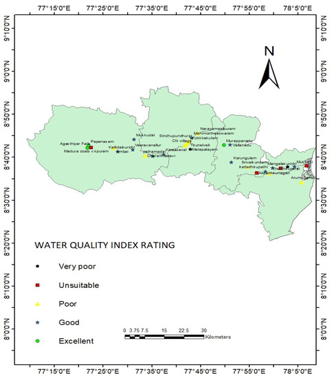
Figure 4.
Water quality suitability map. Source: ArcGIS.
As per [49], the drinking water samples of Villages in Chabahr city, Sistan, and Baluchistan of Iran were tested for their water quality indices. They claimed that 25% of the water was excellent, 50% was good, and 25% was of poor quality.
3.2.1. Factor Analysis of Zone 1 (Ambasamudram Taluk)
The total variance behavior of this zone is provided in Table 6. From this, it is evident that there is an 86.128 percent cumulative variance throughout the season. The first component has a 37.357 percent variance and the second component accounts for 20.820 percent variance. The third component has a variance of 15.035, whereas the fourth component covers 12.915% variance.
Table 6.
Total variance behavior of Zone 1.
As per [40], five principal components (PC) were obtained for a water quality assessment study in the Acude Macela reservoir, Brazil. They claimed that PC1 accounts for 25.57% of variance, PC2 for 13.60% variance, PC3 for 12.36% variance, PC4 for 10.61% variance, and PC5 for 10.05% variance, covering a total of 72% variance. They concluded that the presence of nitrogen and high levels of salinity were the main contributors to high pollution.
The parameters that account for every component discussed above are provided in detail in the rotated component matrix, which is provided in Table 7. From Table 7, it is evident that pH, Ca, HCO3, and F all influence the first component, which has a 37.357 percent variance. The positive coordination between pH and HCO3 can be attributed to the dominance of the alkalinity factor [50]. Na, Mg, and K all influence the second component, which has a variance of 20.820 percent. Higher TH and SO4 influence the third component, which has a variance of 15.035, whereas NO3 negatively dominates the fourth component, which covers 12.915% variance. These higher loadings of these components can be linked to the mineral components of the water.
Table 7.
Rotated component matrix for Zone 1. (Extraction method—Principal Component Analysis; Rotation method—Varimax with Kaiser Normalization; Rotation converged in seven iterations).
The Eigen value of a factor indicates its significance. The components with Eigen values greater than one are considered significant [42]. The scree plot analysis for this zone is provided in Figure 5. From the variance behavior studies discussed above, it was determined that the first four components are significant. This is being evidenced with this scree plot provided in Figure 5. From this scree plot, it is evident that the first four components have Eigen values greater than one and hence these are significant ones to consider for the variance analysis [41].
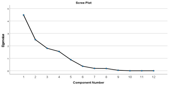
Figure 5.
Screen plot analysis of Zone 1 (Ambasamudram taluk). Source—output from IBM SPSS 28.0.
3.2.2. Factor Analysis of Zone 2 (Tirunelveli Palayamkottai Taluks)
The total variance behavior of Zone 2 is provided in Table 8. From this, it is evident that there is an 80.158 percent cumulative variance throughout the season. The primary component has 37.915 percent variance and the second component accounts for 24.220 percent variance. The third component has a variance of 18.024 percent.
Table 8.
Total variance behavior of Zone 2.
The parameters that account for every component discussed are provided in detail in the rotated component matrix that is provided in Table 9. From Table 9 it is evident that K, Ca, TDS, and SO4 influence the first component, which has a 37.915 percent variance. The NO3 influence the second component, which has a variance of 24.220 percent. The higher loadings of Ca, SO4, Mg, and K indicate the urban waste disposal and high levels of nitrate can be well attributed to the usage of fertilizers for agriculture in that zone [50]. The TH influence the third component, which has a variance of 18.024 percent and can be attributed to the TH.
Table 9.
Rotated component matrix for Zone 2 (Extraction method—Principal Component Analysis; Rotation method—Varimax with Kaiser Normalization; Rotation converged in four iterations).
The scree plot analysis for this zone is provided in Figure 6. From the variance behavior studies discussed above and the screen plot it was determined that the first three components are significant for this zone.
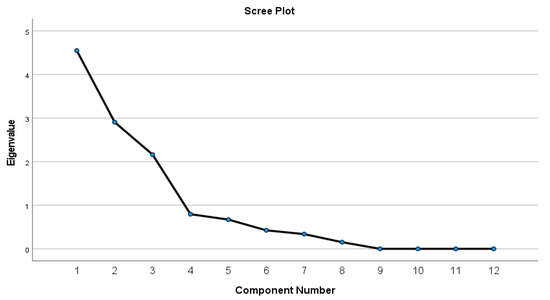
Figure 6.
Screen plot analysis of Zone 2 (Tirunelveli/Palayamkottai) Taluks. Source—output from IBM SPSS 28.0.
3.2.3. Factor Analysis of Zone 3 (Srivaikundam Taluk)
The total variance of this zone is explained in Table 10. As per this reading, it is observed that the cumulative variance of 87.976 percent prevails for the zone. The first component has a 36.583 percent variance, whereas the second component is responsible for a variance of 28.057 percent. The third component accounts for a variance of 12.902 and the last significant component covers 10.435% variance.
Table 10.
Total variance behavior of Zone 3.
The parameters that account for every component is provided in detail in the rotated component matrix in Table 11. From Table 11, it is known that Mg, Cl, TH, and Ca all contribute to the first component, which has a 36.583 percent variance. This indicates the presence of alkaline earth metals and the urban waste disposal in this zone. pH, TDS, and Ca all influence the second component, which has a variance of 28.057 percent. Higher HCO3 and TH influence the third component that has a variance of 12.902. SO4 dominates the fourth component that covers 10.435% variance.
Table 11.
Rotated component matrix for Zone 3 (Extraction method—Principal Component Analysis; Rotation method—Varimax with Kaiser Normalization; Rotation converged in six iterations).
From the variance behavior studies discussed above, it was determined that the first four components are significant. This is being proved again with this scree plot provided in Figure 7. From this scree plot, it is evident that the first four components have Eigen values more than one and hence these are significant ones to consider for the variance analysis.
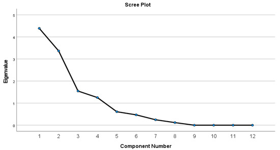
Figure 7.
Screen plot analysis of Zone 3 (Srivaikundam Taluk. Source—Output from IBM SPSS 28.0).
3.2.4. Factor Analysis of Zone 4 (Tiruchendur Taluk)
Table 12 shows the total variance explained for Zone 4. From this variance table, it is inferred that there exists a 91.242 percent cumulative variance throughout the season. There are three significant components observed in this zone. The first component accounts for 47.059 percent variance. The second component is responsible for a variance of 27.945 percent and the third one for 16.239 percent variance.
Table 12.
Total variance behavior of Zone 4.
With these three components, the rotated component matrix is derived. Table 13 shows the rotated component matrix. It is inferred that Cl, Nitrate, and Na all influence the first component, which has a 47.059 percent variance. This variance coverage is almost half of the total variance and the high levels of Na and Cl can be very well attributed to the salinity factor. TDS, K, and HCO3 all influence the second component, which has a variance of 27.945 percent. SO4 negatively impacts the third component, which has a variance of 16.239.
Table 13.
Rotated component matrix for Zone 4. (Extraction method—Principal Component Analysis; Rotation method—Varimax with Kaiser Normalization; Rotation converged in four iterations).
Figure 8 shows the Scree plot analysis of Zone 4. It is indicated that three components are having Eigen values more than 1 and these are of higher significance.
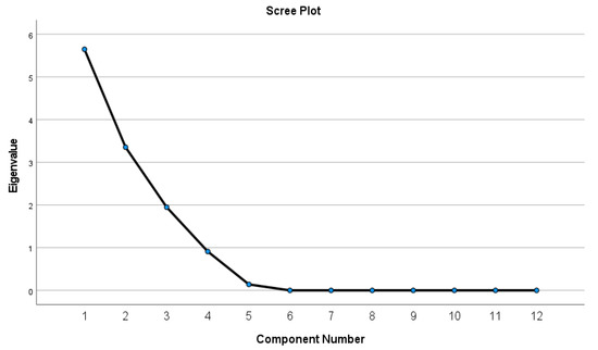
Figure 8.
Screen plot analysis of Zone 4 (Tiruchendhur Taluk). Source—Output from IBM SPSS 28.0.
4. Conclusions
This study is focused on the water quality assessment of the Thamirabarani river basin in south India. Few water quality studies have been conducted in this river basin so far and no major study has applied a multivariate approach similar to PCA to assess the water quality of this basin.
The hydro-geochemical analysis showed that the water in the Thamirabarani River basin is fresh to brackish as well as alkaline, which makes it good for drinking and farming. At most of the sampling sites, the water quality in Thamirabarani is good —average, but alarming levels of pollutants were observed in stations such as V.K. Puram, Tirunelveli, C.N. Village, Alwarthirunagari, and Cheranmahadevi. In these stations, urban sewage disposal and high levels of runoff from agricultural fields are observed. It has been observed that certain locations such as Eral, Punnaikayal, and Senthapoo mangalam have saline pockets due to the proximity of the Bay of Bengal. These sites have maximum levels of chemicals, which are unfit for drinking or irrigation use.
Spatial interpolation maps were prepared to get a clear idea of the variability of chemical composition over the entire study area.
The water quality index studies were conducted and it was revealed that 15% of the water samples are excellent, 35% are fit for potable use, 25% are poor, 15% are very poor, and 10% are unfit for consumption.
The Principal Component Analysis technique was applied to the parameters studied and a detailed zone-wise analysis was performed. It was revealed that Zone 1 is influenced mainly by the alkalinity factor. No major quality issues were inferred from this zone. In Zone 2, K, Ca, TDS, and SO4 are the major influencing components, this can be well attributed to the anthropogenic and industrial activities in the area that discharge waste outlets to the river. Additionally, high positive loadings of Nitratesmay may be attributed to the high usage of fertilizers in that area. In Zone 3, Ca and Mg have a greater positive loading along with TH. This feature can be well attributed to anthropogenic activities and the hardness of the water. In Zone 4, Na, Cl, Nitrate, and F form the major components that determine the quality of river water. More Na and Cl are well attributed to the seawater intrusion in this zone [50].
Reference [51] concluded that three factors were predominant in the water quality assessment of the Lower Bhavani River basin. They claimed that Factor 1 is influenced by anthropogenic and natural sources, Factor 2 is influenced by K and SO4, and Factor 3 is dominated by F and Ca.
Reference [52] conducted a spatial variation analysis of the Malacca River water quality and concluded that six components in Cluster 1 and eight components in Cluster 2 were identified as major PCs. They claimed that agricultural activities and sewage disposal are the main contributors to Cluster 1 and Cluster 2, respectively.
The overall water quality in the Thamirabarani River Basin is influenced by anthropogenic and natural sources of pollution. It is recommended that industries invest in zero effluent discharge and that a proper urban waste management system be planned to minimize sewage disposal. It is recommended to build an efficient water treatment system in the saline area to safeguard the water quality for the people in the threatened regions.
5. Scope for Future Research
Zone-wise and parameter-wise Hierarchical Cluster analysis of water quality can be conducted in this study area.
The water pollution in stations such as Cheranmahadevi, V.K. Puram, and Ambasamudram can be researched deeper so that every single pollution contributor can be identified.
Similar multivariate analysis can be performed for the tributaries of the Thamirabarani River such as Servalar, Kadananathi, Pachaiyar, Chittar, and Ramanathi.
Author Contributions
Conceptualization, E.T. and M.A.; methodology, E.T.; software, E.T.; validation, A.S.; formal analysis, E.T. and M.A.; investigation, E.T. and A.S.; resources, E.T., R.P. and C.C.; data curation, E.T.; writing—original draft preparation, E.T. and A.S.; writing—review and editing, E.T., A.S. and R.P.; visualization, E.T. and M.A.A.; supervision, E.T. and M.A.; project administration, E.T., M.A. and E.S.F.; funding acquisition, E.S.F. All authors have read and agreed to the published version of the manuscript.
Funding
E.I. Saavedra Flores acknowledges the financial support from the Chilean National Agency for Research and Development (ANID), research grant FONDECYT REGULAR No.1211767.
Institutional Review Board Statement
Not applicable.
Informed Consent Statement
Not applicable.
Data Availability Statement
Not applicable.
Acknowledgments
The authors gratefully appreciate the support given by the Research Department of Sathyabama Institute of Science and Technology, Chennai, India. They also appreciate the support given by the Department of Civil Engineering, Alagappa Chettiar Government College of Engineering and Technology, Karaikudi, Tamilnadu, India through TEQIP-III, implemented by the National Project Implementation Unit (NPIU) of the Ministry of Human Resource Development, Government of India.
Conflicts of Interest
The authors declare no conflict of interest.
References
- Phiri, O.; Mumba, P.; Moyo, B.H.Z. Assessment of the impact of industrial effluents on water quality of receiving rivers in urban areas of Malawi. Int. J. Environ. Sci. Technol. 2005, 2, 237–244. [Google Scholar] [CrossRef]
- Venkatramanan, S.; Chung, S.Y.; Lee, S.Y.; Park, N. Assessment of River Water Quality Via Environmentric Multivariate Statistical Tools And Water Quality Index: A Case Study Of Nakdong River Basin, Korea. Carpathian J. Earth Environ. Sci. 2014, 9, 125–132. [Google Scholar]
- Ouyang, Y.; Nkedi-Kizza, P.; Wu, Q.T.; Shinde, D.; Huang, C.H. Assessment of Seasonal Variations in Surface Water Quality. Water Res. 2006, 40, 3800–3810. [Google Scholar] [CrossRef]
- Cui, B.; Yang, Q.; Yang, Z.; Zhang, K. Evaluating The Ecological Performance Of Wetland Restoration In The Yellow River Delta, China. Ecol. Eng. 2009, 35, 1090–1103. [Google Scholar] [CrossRef]
- Yahong, Z.; Peiyue, L.; Leilei, X.; Zihan, D.; Duo, L. Solute geochemistry and groundwater quality for drinking and irrigation purposes: A case study in Xinle City, North China. Geochemistry 2020, 80, 125609. [Google Scholar] [CrossRef]
- Yu, S.; Shang, J.; Zhao, J.; Guo, H. Factor Analysis and Dynamics of Water Quality of the Sanghua River, Northeast China. Water Air Soil Pollut. 2003, 144, 159–169. [Google Scholar] [CrossRef]
- Galezzo, M.A.; Susa, M.R. The challenges ofmonitoring andcontrolling drinking-water quality indispersed rural areas: Acase study based ontwo settlements intheColombian Caribbean. Environ. Monit. Assess. 2021, 193, 373. [Google Scholar] [CrossRef] [PubMed]
- Manoj, K.; Padhy, P.K. Multivariate statistical techniques and water quality assessment: Discourse and review on some analytical models. Int. J. Environ. Sci. 2014, 5, 607. [Google Scholar]
- Hair, J.F.; Black, W.C.; Babin, B.J.; Anderson, R.E.; Tatham, R.L. Multivariate Data Analysis; Prentice Hall: Upper Saddle River, NJ, USA, 1998; Volume 5, pp. 207–219. [Google Scholar]
- Kanade, S.B.; Gaikwad, V.B. A multivariate statistical analysis of bore well chemistry data: Nashik and Niphad Taluka of Maharashtra, India. Univers. J. Environ. Res. Technol. 2011, 1, 193–202. [Google Scholar]
- Aydin, H.; Ustaoğlu, F.; Tepe, Y.; Soylu, E.N. Assessment of water quality of streams in northeast Turkey by water quality index and multiple statistical methods. Environ. Forensics 2020, 22, 270–287. [Google Scholar] [CrossRef]
- Nasirian, M. A new water quality index for environmental contamination contributed by mineral processing: A case study of Amang (Tin Tailing) processing activity. J. Appl. Sci. 2007, 7, 2977–2987. [Google Scholar] [CrossRef]
- Ismail, A.; Robescu, L.D. Chemical water quality assessment of the Danube river in the lower course using water quality indices. U.P.B. Sci. Bull. 2017, 79, 51–61. [Google Scholar]
- Effendi, H.; Wardiatno, R.Y. Water Quality Status of Ciambulawung River, Banten Province, Based on Pollution Index and NSF-WQI. Procedia Environ. Sci. 2015, 24, 228–237. [Google Scholar] [CrossRef]
- Gazzaz, N.M.; Yusoff, M.K.; Aris, A.Z.; Juahir, H.; Ramli, M.F. Artificial neural network modeling of the water quality index for Kinta River (Malaysia) using water quality variables as predictors. Mar. Pollut. Bull. 2012, 64, 2409–2420. [Google Scholar] [CrossRef] [PubMed]
- Rosu, A.; Rosu, B.; Constantin, D.E.; Voiculescu, M.; Arseni, M.; Calmuc, V.; Iticescu, C.; Georgescu, L.P. Overview of NO2 Pollution Level in the Lower Danube Basin during Dans Measurements Campaign. Theor. Mech. 2018, 41, 163–170. [Google Scholar] [CrossRef]
- Brown, R.M.; Mc Clelland, N.I.; Deininger, R.A.; Tozer, R.G. A Water Quality Index—Do We Dare. Water Sew. Work 1970, 117, 339–343. [Google Scholar]
- Saffran, K.; Cash, K.; Hallard, K.; Neary, B.; Wright, R. Canadian water quality guidelines for the protection of aquatic life. CCME Waterquality Index 2001, 1, 1–23. [Google Scholar]
- Adimalla, N. Groundwater quality for drinking and irrigation purposes and potential health risk assessment: A case study from semi-arid region of South India. Expo. Health 2019, 11, 109–123. [Google Scholar] [CrossRef]
- Mohana, P.; Nagamani, K.; Muthusamy, S.; Velmurugan, P.M. Environmental Impact Assessment of Thamirabarani River Basin, Tamil Nadu using Remote Sensing and GIS Techniques. Indian J. Sci. Technol. 2018, 11, 1–7. [Google Scholar] [CrossRef]
- Reymond, D.J.; Sudalaimuthu, K. Geospatial Water Quality Analysis of Downstream of Tamiraparani River—Tamilnadu. J. Eng. Res. 2022. [Google Scholar] [CrossRef]
- Murugesan, A.G.; Mophin-Kania, K. Evaluation and Classification of Water Quality of Perennial River Tamirabarani through Aggregation of Water Quality Index. Int. J. Environ. Prot. 2011, 1, 24–33. [Google Scholar]
- American Public Health Association (APHA). Standard Methods for the Examination of Water and Wastewater, 22nd ed.; American public Health Association: Washington DC, USA, 2012. [Google Scholar]
- Brindha, K.; Elango, L. Groundwater quality zonation in a shallow weathered rock aquifer using GIS. Geo-Spatial Inf. Sci. 2012, 15, 95–104. [Google Scholar] [CrossRef]
- Reddy, A.G.S.; Reddy, D.V.; Rao, P.N.; Prasad, K.M. Hydrogeochemical characterization of fluoride rich groundwater of Wailpalliwatershed, Nalgonda District, Andhra Pradesh, India. Environ. Monit. Assess. 2010, 171, 561–577. [Google Scholar] [CrossRef] [PubMed]
- Ayyandurai, R.; Venkateswaran, S.; Karunanidhi, D. Hydrogeochemical assessment of groundwater quality and suitability for irrigation in the coastal part of Cuddalore district, Tamil Nadu, India. Mar. Pollut. Bull. 2022, 174, 113258. [Google Scholar] [CrossRef]
- Ranjith, S.; Shivapur, A.V.; Kumar, S.K.P.; Chandrashekarayya, G.H.; Dhungana, S. Water Quality Assessment of River Tungabhadra, India. Nat. Environ. Pollut. 2020, 19, 1957–1963. [Google Scholar]
- American Public Health Association (APHA). Standard Methods for the Examination of Water and Wastewater, 20th ed.; American Public Health Association: Washington DC, USA, 2005. [Google Scholar]
- Kumar, P.J.S. GIS-based mapping of water-level fuctuations (WLF) and its impact on groundwater in an Agrarian District in Tamil Nadu, India. Environ. Dev. Sustain. 2021, 24, 994–1009. [Google Scholar] [CrossRef]
- Robinson, A.H.; Morrison, J.L.; Muehrcke, P.C.; Kimerling, A.J.; Guptil, S.C. Elements of Cartography, 6th ed.; John Wiley and Sons: New York, NY, USA, 1995. [Google Scholar]
- Chang, K. Introduction to Geographic Information Systems, 4th ed.; Tata McGraw-Hill: New York, NY, USA, 2012. [Google Scholar]
- Wu, H.W.E.; Hung, M.C. Comparison of Spatial Interpolation Techniques Using Visualization and Quantitative Assessment. In Applications of Spatial Statistics; IntechOpen: London, UK, 2016; pp. 17–34. [Google Scholar] [CrossRef]
- Duraisamy, S.; Govindhaswamy, V.; Duraisamy, K.; Krishinaraj, S.; Balasubramanian, A.; Thirumalaisamy, S. Hydrogeochemical characterization and evaluation of groundwater quality in Kangayam taluk, Tirupur district, Tamil Nadu, India, using GIS techniques. Environ. Geochem. Health 2018, 41, 851–873. [Google Scholar] [CrossRef]
- Ustaoğlu, F.; Taş, B.; Tepe, Y.; Topaldemir, H. Comprehensive assessment of water quality and associated health risk by using physicochemical quality indices and multivariate analysis in Terme River, Turkey. Environ. Sci. Pollut. Res. 2021, 28, 62736–62754. [Google Scholar] [CrossRef]
- Chaurasia, A.K.; Pandey, H.K.; Tiwari, S.K.; Prakash, R.; Pandey, P.; Ram, A. Groundwater quality assessment using water quality index (WQI) in parts of Varanasi District, UttarPradesh, India. J. Geol. Soc. India 2018, 92, 76–82. [Google Scholar] [CrossRef]
- Rabeiy, R.E. Assessment and modeling of groundwater quality using WQI and GIS in Upper Egypt area. Environ. Sci. Pollut. Res. 2017, 25, 30808–30817. [Google Scholar] [CrossRef]
- Ichwana, I.; Syahrul, S.; Nelly, W. Water Quality Index by Using National Sanitation Foundation-Water Quality Index (NSF-WQI) Method at Krueng Tamiang Aceh. In Proceedings of the International Conference on Technology, Innovation, and Society (ICTIS), Padang, India, 21–22 July 2016. [Google Scholar] [CrossRef]
- Murugesan, V.; Krishnara, S.; Vijayaragavan, K.; Ganthi, R.R. Application of water quality index for groundwater quality assessment: Thirumanimuttar sub-basin, Tamilnadu, India. Environ. Monit. Assess. 2010, 171, 595–609. [Google Scholar]
- Nasir, M.F.M.; Samsudin, M.S.; Mohamad, I.; Awaluddin, M.R.A.; Mansor, M.A.; Juahir, H.; Ramli, N. River Water Quality Modeling Using Combined Principle Component Analysis (PCA) and Multiple Linear Regressions (MLR): A Case Study at Klang River, Malaysia. World Appl. Sci. J. 2011, 14, 73–82. [Google Scholar]
- Garcia, C.A.B.; Garcia, H.L.; Mendonça, M.C.S.; Silva, A.F.; Alves, J.P.H.; Costa, S.S.L.; Araújo, G.O.; Silva, I.S. Assessment of water quality using principal component analysis: A case study of the açude da Macela—Sergipe—Brazil. Mod. Environ. Sci. Eng. 2017, 3, 690–700. [Google Scholar] [CrossRef]
- Tao, X.F.; Huang, T.; Li, X.F.; Peng, D.P. Application of a PCA based water quality classification method in water quality assessment in the Tongjiyan Irrigation Area, China. In Proceedings of the International Conference on Energy and Environmental Protection (ICEEP), Sanya, China, 21–23 November 2016; pp. 118–125. [Google Scholar] [CrossRef]
- Bhat, S.A.; Meraj, G.; Yaseen, S.; Pandit, A.K. Statistical Assessment of Water Quality Parameters for Pollution Source Identification in Sukhnag Stream: An Inflow Stream of Lake Wular (Ramsar Site), Kashmir Himalaya. J. Ecosyst. 2014, 2014, 898054. [Google Scholar] [CrossRef]
- Gupta, N.; Pandey, P.; Hussain, J. Effect of physicochemical and biological parameters on the quality of river water of Narmada, Madhya Pradesh, India. Water Sci. 2017, 31, 11–23. [Google Scholar] [CrossRef]
- Gnanachandrasamy, G.; Dushiyanthan, C.; Rajakumar, T.J.; Zhou, Y. Assessment of hydrogeochemical characteristics of groundwater in the lower Vellar river basin: Using Geographical Information System (GIS) and Water Quality Index (WQI). Environ. Dev. Sustain. 2018, 22, 759–789. [Google Scholar] [CrossRef]
- Davis, S.N.; De Weist, R.J.M. Hydrogeology; John Wiley and Sons: New York, NY, USA, 1966; p. 463. [Google Scholar]
- Freeze, R.A.; Cherry, J.A. Groundwater; Prentice-Hall: Hoboken, NJ, USA, 1979; 604p. [Google Scholar]
- Reddy, B.M.; Sunitha, V. Geochemical and health risk assessment of fluoride and nitrate toxicity in semi-arid region of Anantapur District, South India. Environ. Chem. Ecotoxicol. 2020, 2, 150–161. [Google Scholar]
- Saxena, U.; Saxena, S. Correlation Study on Physico-Chemical Parameters And Quality Assessment Of Ground Water Of Bassi Tehsil Of District Jaipur, Rajasthan, India, Suresh Gyan Vihar University. Int. J. Environ. Sci. Technol. 2015, 1, 78–91. [Google Scholar]
- Abbasnia, A.; Alimohammadi, M.; Mahvi, A.H.; Nabizadeh, R.; Yousefi, M.; Mohammadi, A.A.; Pasalari, H.; Mirzabeigi, M. Assessment of groundwater quality and evaluation of scaling and corrosiveness potential of drinking water samples in villages of Chabahr city, Sistan and Baluchistan province in Iran. Data Brief 2018, 16, 182–192. [Google Scholar] [CrossRef]
- Rao, N.S.; Rao, J.P.; Subrahmanyam, A. Principal Component Analysis in Groundwater Quality in a Developing Urban Area of Andhra Pradesh. J. Geol. Soc. India 2007, 69, 959–969. [Google Scholar]
- Kumar, P.J.S. Hydrogeochemical and multivariate statistical appraisal of pollution sources in the groundwater of the lower Bhavani River basin in Tamil Nadu. Geol. Ecol. Landsc. 2020, 4, 40–51. [Google Scholar] [CrossRef]
- Hua, A.K.; Kusin, F.M.; Praveena, S.M. Spatial Variation Assessment of River Water Quality Using Environmetric Techniques. Pol. J. Environ. Stud. 2016, 25, 2411–2421. [Google Scholar] [CrossRef] [PubMed]


Publisher’s Note: MDPI stays neutral with regard to jurisdictional claims in published maps and institutional affiliations. |
© 2022 by the authors. Licensee MDPI, Basel, Switzerland. This article is an open access article distributed under the terms and conditions of the Creative Commons Attribution (CC BY) license (https://creativecommons.org/licenses/by/4.0/).