Abstract
To obtain an accurate one-dimensional velocity model, we developed the EA_VELEST method based on the evolutionary algorithm and the VELEST program. This method can quickly generate a suitable 1D velocity model and finally input it into the 3D velocity inversion process using the TomoDD method. We adopt TomoDD methods to inverse the high-resolution three-dimension velocity structure and relative earthquake hypocenters for this sequence. This system processing flow was applied to the Sichuan Maerkang earthquake swarm in 2022. By collecting the seismic phase data of the Maerkang area between 1 January 2009 and 15 June 2022, we relocated the historical earthquakes in the area and obtained accurate 3D velocity imaging results. The relocated hypocenters reveal a SE-trending secondary fault, which is located ~5 km NW of the Songgang fault. In the first ten-hour of the sequence, events clearly down-dip migrated toward the SE direction. The inverted velocity structure indicates that the majority of earthquakes during the sequence occurred along the boundaries of the high and low-velocity zones or high and low-VP/VS anomalies. Especially both the two largest earthquakes, MS 5.8 and MS 6.0, occurred at the discontinuities of high and low-velocity zones. The EA_VELEST method proposed in this paper is a novel method that has played a very good enlightenment role in the optimization of the one-dimensional velocity model in geophysics and has certain reference significance. The 3D velocity results obtained in this paper and the analysis of tectonic significance provide a reference for the seismogenic environment of this Maerkang earthquake and the deep 3D velocity of the Ganzi block.
1. Introduction
Earthquake is a major natural disaster, seriously endangering the sustainable development of society and the economy [1,2,3]. There are many methods for earthquake research; the most direct is to understand the internal structure of the underground and the physical properties of the fault. Seismic tomography technology is widely used in the study of the earth’s internal structure and has achieved fruitful research results [4,5,6,7,8,9,10,11]. Seismic tomography is a geophysical method [12,13,14,15] that reverses important information such as velocity structure and other physical parameters of underground media by analyzing the observed data of kinematic (such as travel time, ray path) and dynamic (such as waveform, amplitude) characteristics of various seismic phases of seismic waves. However, in order to obtain an accurate three-dimensional velocity structure, an accurate one-dimensional velocity model is first constructed, and then a 3-D tomographic imaging model is usually obtained in the form of 1-D reference model perturbation. An accurate one-dimensional velocity structure is the premise of the accurate earthquake location to avoid getting the wrong source position. Improper selection of the velocity model, even if a double difference precision positioning method is used [16], will lead to significant distortion and deviation of source position. Tomographic results and resolution estimates largely depend on the selection of initial models. Inadequate reference models may actually cause serious deformation of tomographic images or introduce artifacts, leading to a misunderstanding of the results [17]. In areas with strong lateral variation and irregular terrain surfaces, the systematic migration of significant errors or seismic positions can be solved by using simplified one-dimensional velocity parameterization. The one-dimensional velocity inversion method VELEST [18] is an enduring method and is widely used. The accurate one-dimensional velocity model obtained by selecting certain reliable seismic events is conducive to improving the accuracy of seismic location and tomography. It plays a unique role in the correction of velocity models in regions with complex tectonic settings. To obtain reliable results, VELEST needs a wide range of calculations, randomly perturbs the initial speed model, and finally selects the optimal model by relying on the average root mean square of travel time(RMS) [18,19,20,21]. This process is a time-consuming process. In this paper, we propose a simple and fast one-dimensional velocity calculation method based on the optimization algorithm EA (Evolutionary Algorithm) and apply it to the case study of the 2022 Sichuan Maerkang earthquake swarm in China in combination with the double difference tomographic TomoDD method [22,23]. Finally, based on the obtained 3D velocity inversion results and geological structure conditions, a detailed discussion is carried out.
2. The Background and Regional Tectonic Background of the Maerkang Earthquake Swarm
According to the official determination of the China Earthquake Network Center, an MS 5.8 (32.28° N, 101.79° E), an MS 6.0 (32.25° N, 101.82° E) and an MS 5.2 (32.24° N, 101.85° E) earthquake occurred at 0:21, 1:28 and 3:27, respectively, in Maerkang, Aba Prefecture, Sichuan, on 10 June 2022 [24,25]. According to the type of earthquake sequence, this earthquake is a swarm type, and the successive earthquakes of MS 5.0 or higher caused a certain superposition of earthquake damage. The highest intensity of the earthquake is VIII (8 degrees). The main area is located in Caodeng Township, the epicenter of the earthquake. The surrounding areas, such as Chengdu, Deyang, Mianyang, Ya’an, etc., are obviously affected by the earthquake, causing certain social impacts. Other lifeline projects, such as roads, electric power, and communications in the epicenter area, were also severely damaged in the earthquake (https://www.sc.gov.cn/10462/10464/13722/2022/6/13/6e77cbec7ee14bb29fad35c4cd156a94.shtml, accessed on 9 November 2022). When an earthquake reaches a certain magnitude, its signal is easy to be received by the seismic observation instrument [26], and the seismic staff can obtain the seismic catalog data according to the analysis of the seismic signal. According to the earthquake catalog of the China Seismological Network Center, as of 0:00 on 16 June 2022, there were 2694 aftershocks in the Sichuan Maerkang earthquake, including 7 MS 3.0–MS 4.0 aftershocks, 4 MS 4.0–MS 5.0 aftershocks, and 2 above MS 5.0 aftershocks. Aftershocks are relatively developed. Considering that the epicenter is located in the mountain valley area on the southern edge of the Northwest Sichuan Plateau, the terrain is characterized by high mountains, deep valleys, and steep slopes. The rock mass on the mountain is relatively loose. Affected by the local geological conditions, the earthquake is likely to trigger secondary geological disasters such as landslides, rolling stones, and collapses. Therefore, it is of great significance to determine the precise location of the earthquake source and the seismogenic fault in time.
Only 21 km to the northwest of this earthquake, an ML 5.0 earthquake (32.3° N, 101.58° E) occurred on 5 January 2005. Similar to this earthquake sequence, the two earthquakes are swarm earthquakes, with a certain foreshock and rich aftershock sequence [27,28]. The cumulative variation of the regional gravity field in western Sichuan shows that a high gradient zone of gravity variation along the NNW direction is formed between Maerkang and Lushan areas [29]. Therefore, the analysis and study of the earthquake occurrence background in this region will help to provide the scientific basis for future study and judgment of earthquake risk. To explore the deep background of the occurrence of this earthquake and the precise spatial distribution of the seismic sequence, this paper downloads and uses the seismic observation reports of this earthquake sequence and the surrounding area given by the China Earthquake Network Center and performs a case study of the 10 June 2022 Maerkang earthquake swarm based on the double-difference tomography method [22] for precise location and tomography processing. Seismic location is a basic problem in seismology. High-resolution source locations can identify and outline the geometry of buried faults [30,31]. The three-dimensional velocity structure of the source region is a reliable basis for us to explore the deep seismogenic environment and understand the medium information.
The Bayankala block, where strong earthquakes are concentrated in the Chinese Mainland, can be further divided into two sub-blocks by the Longriba fault: the Aba sub-block and the Longmenshan sub-block [32]. The Maerkang earthquake is an intra-plate earthquake within the Aba sub-block, which is usually of a smaller magnitude compared to earthquakes at plate boundaries. Tectonically, the Aba sub-block is surrounded by the Longriba Fault Zone to its east, the East Kunlun Fault to its northeast, and the Xianshui River Fault to its southwest, and its movement is strictly controlled by the three boundary faults [33]. The Longriba fault, located to the southeast of the epicenter, is almost parallel in the strike to the Longmenshan fault to the east of the epicenter and is 200 km apart, showing a right-lateral strike-slip and thrust nature [33], with a slip rate of ~7.5 mm/yr in the Late Pleistocene and ~2.1 mm/yr in the Holocene [34].
Songgang–Fubian River fault, Maduo–Gande fault, Gande South fault and Aba fault zone are developed in the Aba sub-block (Figure 1). This earthquake occurred near the Songgang–Fabian River Fault. The Songgang–Fubian River Fault can be divided into the Songgang Fault in the NW section and the Fubian River Fault in the SE section. Among them, the Songgang Fault is NW-trending and is spreading in the NW–SE direction. The seismic activity of the rupture is inactive in the northern section, with deep, viscous slip and surface locking in the middle section, and more active in the southern section, with obvious segmentation [35]. The sliding rate of the rupture near the Culuchang is 1.7 mm/a [36]. The Fubian River Fault is located in the southeast of the Songgang Fault and is connected to the Songgang Fault at the west end, spreading in a NW–SE direction, with a right-lateral strike-slip and thrust nature and a segmented horizontal sliding rate of ≥0.85 mm/a near Majiagou and higher than 1.7 mm/a near Niuqiangou [33]. The Aba Fault spreading direction is northwest-southeast, including the Aba Basin North Rim Fault, South Rim Fault, and Central Fault, all composed of several branching composite faults, and this fault is a very important branching fault in the eastern section of the Maduo–Gande Fault.
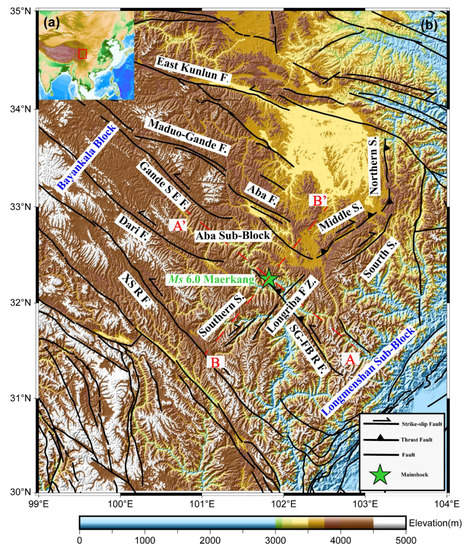
Figure 1.
Tectonic background of the study area. (a) represents the distribution of the study area in China. (b) represents the tectonic background area of the study area. (red dashed lines AA ‘and BB’ are the strike and vertical sections along the Maerkang earthquake sequence, respectively, faults data source: https://www.activefault-datacenter.cn, accessed on 9 November 2022).
3. Dataset and Methods
3.1. Dataset
The earthquake catalog and seismic phase reports used in the study are the Uniform Official Catalog and Official Observation Report provided by the Seismic Cataloging System of the China Earthquake Network Center. The data span from 1 January 2009 to 15 June 2022, and the starting and ending times correspond to the completion of the digital seismic network renovation in the “Fifteen Plan” of the China Seismic Network and the fifth day after the 2022 Sichuan Maerkang MS 6.0 earthquake, respectively. The seismic events with epicenter distance < 500 km and recorded by at least three stations at the same time were selected to ensure the quality of seismic data.
During the period from 1 January 2009 to 15 June 2022, a total of 9373 initially located seismic events meeting the above selection conditions in the seismic location and tomography study area (31°–34° N, 100°–103° E, hereafter referred to as the study area) with magnitudes ranging from ML-0.6 to MS 6.0. In order to make the seismic rays fully cover the study area, this paper takes the MS 6.0 Maerkang earthquake as the center and extends 1.5° outward as the tomography inversion area, using 119 regional fixed seismic stations in the range of 99°~104° E and 30°~35° N (Figure 2). Figure 2 shows the distribution of seismic stations and seismic rays. From the figure, the ray distribution shows that most of the coverage in the study area is intact, and the ray coverage is poor in the northwest Qinghai area due to the sparsity of seismic stations. The ray coverage is poor in the northwest Qinghai region due to the sparsity of seismic stations. The depth profile shows ray distribution rate above 30 km depth has a high coverage rate. It is worth mentioning that the ray paths are plotted as simple straight-line paths, which are somewhat different from the ray paths in the actual inhomogeneous crustal velocity model, and are only used for reference.
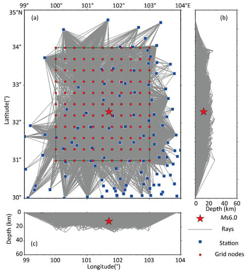
Figure 2.
Station and three-dimensional ray distribution used in this paper. (a) shows the distribution of ray nodes in the horizontal area. (b) shows the ray distribution at latitude and depth. (c) shows the ray distribution in longitude and depth. (red five-pointed star represents the location of MS 6.0 main shock, the blue box represents seismic station, red origin represents the set of grid nodes, and the green rectangle represents the study area).
3.2. Method Introduction
Seismic location and inversion of the crustal velocity structure are critical issues in understanding the mechanism of earthquake occurrence and locating the seismogenic faults [37]. The 1D crustal velocity structure is a critical factor in determining the accuracy of seismic localization. However, the spatial uniqueness of the subsurface medium leads to significant differences in the velocity structure in different regions, so it is necessary to develop a specific 1D velocity model to be used as the initial velocity model for location or tomography according to the study area [38,39]. Because the initial location of the seismic observation report uses a simple one-dimensional horizontal layered velocity model, and the reliability of the source depth using the simplex method is poor, we used two steps to obtain a relatively accurate seismic source location in the area of this occurrence: (1) The optimal 1D velocity model is inverted using the VELEST method [18], and the absolute locations of the earthquakes are improved based on the updated 1D velocity model; (2) based on the absolute locations of the earthquakes are improved by VELEST, the updated 1D velocity model, and the seismic phase data, the relative locations of these earthquakes are further determined using the double-difference tomography (TomoDD) method [22,23] for the relative location of these earthquakes.
3.2.1. One-Dimensional Velocity Model and Seismic Absolute Location Optimization
The VELEST algorithm uses the FORTRAN77 programming language and is used to obtain a one-dimensional velocity structure model that matches the geological structural characteristics of the study area. The resulting 1D velocity model can be used as a reference model to improve seismic location accuracy and for seismic tomography. The VELEST algorithm requires an initial velocity model to be selected, and the initial velocity model is continuously modified by correcting the station and source parameters [18]. The one-dimensional velocity model is solved as follows:
The velocity model m satisfies a nonlinear relationship with the seismic wave travel time tabs, station coordinates s, and source parameters h:
As with other time-location methods, seismic wave time data and station information are required to solve the velocity model based on both data. An appropriate 1D velocity structure model is introduced to solve the equation, and then the theoretical travel time tcal of seismic waves is calculated based on ray-tracing theory. By doing the first-order Taylor expansion of Equation (1), the linear relationship between the travel time residual tres and the velocity model correction and source correction can be obtained as follows:
where m is the velocity model parameter vector, h is the seismic source parameter vector, and e is the error vector. In the matrix, the parameter relations in the coupled seismic source parameter model can be written as:
When multiple events are retrieved and located at the same time, the accuracy of the results is evaluated by the root mean square residual(RMS residual) of travel time.
3.2.2. TomoDD Method Introduction
TomoDD is a recursive version of HypoDD [16] that simultaneously solves the 3D velocity structure and seismic event location. TomoDD uses absolute and differential seismic phase walk times to invert the velocity structure in layers of different sizes. The method generates the velocity structure by identifying the incident location closer to the source region, while the standard laminar imaging algorithm uses only absolute seismic phase walk times [22]. It is based on the HypoDD [16] code, which enables the joint inversion of the source location and velocity structure by using absolute and relative seismic phase data. This method determines a three-dimensional velocity model with absolute and relative event locations. This method has the advantage of including relative and absolute epoch travel times in the weights, thus simplifying assumptions about ray path geometry or path anomalies without losing valuable information, using absolute locations, but also modifying absolute positions with iterations [22]. The inversion is performed using an iterative damped least squares technique to solve the linearized, coupled seismic source velocity problem. For standard tomography, the event locations are uncertain and slightly scattered due to errors. TomoDD uses different seismic phase data between adjacent seismic pairs to largely eliminate path effects and thus better invert the velocity structure of the source area [22], so the velocity model obtained by the TomoDD method is, to some extent, superior to standard tomography.
The main principle of the TomoDD method is that the difference between the observed travel time and the theoretical travel time of the seismic rays generated by seismic event i reaching station k can be expressed as the following integral form:
The above equation denotes the seismic wave travel time of seismic event i recorded at station k. is the perturbation value of the source parameter of seismic event i in three different directions, is the perturbation at the moment of seismic i, and δu is the slow perturbation of seismic wave. In addition, the difference between the theoretical and observed travel times of adjacent earthquakes i and j can be expressed as:
The velocity structure of the small-scale range near the earthquake epicenter and the relative source location can be obtained according to Equation (5).
4. Inversion Process and Results
The accuracy of 3D velocity inversion mainly depends on the number of earthquakes and seismic phases, the size of the grid node settings, and the goodness of the initial velocity model [39]. Theoretically, the denser the nodes are, the higher the inversion accuracy is. However, in the case of insufficient data, the denser the nodes are, the lower the node ray coverage will be, and the inversion accuracy will be reduced. In careful consideration, the nodes in this paper are set every 0.3° horizontally, and the depth is set at −3, 0, 3, 6, 9, 12, 15, 20, 25, 30, 35, and 40 km. The speed values outside the nodes are interpolated linearly [40]. See Figure 2 for the horizontal grid nodes. In the seismic location calculation, we set the epicenter spacing of 30 km as the event pair selection threshold, and a single earthquake can form a pair with up to 10 earthquakes. In the selection of damping coefficients and smooth factors in this paper, the L-curve equilibrium curve method [41] is used to make the variance of the data small while ensuring that the amount of variation in the solution does not increase severely. And finally, 150 and 30 are chosen respectively. The initial 1D velocity model is selected as the best model obtained by VELEST optimization.
4.1. VELEST Relocation and One-Dimensional Velocity Optimization Based on EA (Evolutionary Algorithm)
Before setting the initial three-dimensional velocity model, it is often necessary to debug the one-dimensional velocity model. Here, we apply the traditional method VELEST to optimize the one-dimensional velocity model and relocate the earthquake. Traditional methods plus some machine learning optimization methods will achieve better results, which is of great significance in improving the efficiency of traditional methods and algorithms [42,43]. In order to quickly obtain the optimal one-dimensional velocity model, we use the initial velocity model for random perturbation and then use the EA Algorithm 1 to select the optimal one-dimensional velocity model with the minimum RMS calculation. We selected 400 seismic events above ML 2.5 from 9373 events. In the setting of the stochastic model, we refer to the previous research results of the one-dimensional velocity model in this area [44]. After 60 generations of searching for the optimal solution of VELEST, we obtained the optimal 1D velocity model. The results are shown in Table 1. We only need to fill in the required parameters of EA, then set the quality evaluation criteria of the optimal 1D velocity model as the objective function, and wait for the iterative search results. The pseudo-code for this procedure is as follows, and the corresponding source code is available at https://github.com/ECNU-Cross-Innovation-Lab/EA_VELEST, accessed on 9 November 2022.
| Algorithm 1: EA_VELEST |
| Input:vel set’s upper and lower limits, fitness function: VELEST method’s RMS resudial Parameter: Population size S, generation number N, crossover probability , mutation probability Output: the vel set of the target 1D velocity model randomly generate ’s individuals For to S do calculate each individual’s fitness For to N do select; crossover if ; mutation if ; For to S do vel = calculate fitness End for End for Return target model’s vel set |

Table 1.
Initial velocity model and optimal one-dimensional velocity model for absolute positioning using the Velest method and EA.
Our objective function is the minimum RMS residual of the VELEST method. Firstly, appropriate parameters are preset for EA, which are search algebra, N, population size, M, crossover probability, and mutation probability, . Among them, the search algebra is the optimal generation number, and population size is the number of parallel solutions for each generation. Then, the velocity parameters of the 1D velocity model are set as variables to be optimized, which are converted into chromosomes which are the coded representation of the individual in question in the form of a string. Then coded chromosomes to complete the initialization of the population . The parameters at different depths of each group of 1D velocity models correspond to an individual in the population and also to a . Then input the parameters corresponding to each chromosome in into the VELEST method, and calculate their RMS residual, which is also called target function . Next, calculate the probability of each chromosome being selected and choose them by roulette. For the selected chromosomes, they will be randomly paired and crossed at random points if and only if the random crossover probability is larger than . When and only when the probability of random variation is larger than , random variation occurs at the corresponding gene locus. After the above steps, a new generation of the population will be generated. Repeat the above process until the preset search algebra is reached. Finally, after iteration, the velocity corresponding to the minimum RMS residual value of the VELEST model output after model comparison corresponds to the best 1D velocity model found. Since it has been confirmed that excellent results can be obtained when searching the 60-generation population, Figure 3 shows the results of 4 runs of the 60-generation EA operation, which shows that the best 1D speed model obtained is robust. Specifically, Figure 3a shows four variation curves of the RMS residual change effect of 60 generations of EA iteration that can describe the average level of the model during the experiment. It can be seen from the figure that the RMS residual of the best 1D velocity model obtained by EA and VELEST methods are both around 0.1745, and the effect is robust. Moreover, Figure 3b shows the models’ P-velocity and S-velocity corresponding to the above four groups of parameters for comparison.
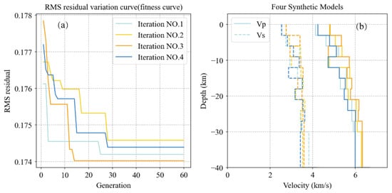
Figure 3.
The results of the four operations of EA_VELEST. (a) Four RMS residual variation curves (fitness curves) with 60 generation EA iteration. (b) 1D Velocity models corresponding to four groups of parameters. The solid line represents the P-wave velocity, and the dotted line represents the S-wave velocity. The lines with four different colors represent four groups of tests, which is consistent with (a).
From the results of the four operations, the models obtained from the four inversions at a depth of 6–15 km in the seismic concentration area are relatively close, indicating that the method proposed in this paper is relatively reliable in obtaining accurate one-dimensional velocity models. It is worth mentioning that, in the depth interval with less seismic distribution, the one-dimensional velocity model obtained by each attempt is relatively different. This paper will further optimize the inversion of the three-dimensional velocity model. Here we choose a set of parameters with an RMS residual of 0.174392, that is, the parameters corresponding to Iteration No. 4 in the figure, which can approximately represent the average level of model parameters after EA iteration. The parameters of the optimal 1D velocity model are shown in Table 1. Compared with the initial 1D velocity model, the overall VP/VS value of the 1D velocity model optimized by the VELEST method in this paper is lower, which is mainly because the initial velocity model is located in the area of southern Sichuan [44]. Wang et al. (2003) [45] proposed that the velocity structure of the adjacent Ganzi block in the study area of this paper has lower values, and the crust of the Tibetan Plateau has softer characteristics. Their study area is adjacent to and partially overlaps with the study area of this paper, which indicates that the inversion results are accurate and reliable. After obtaining the new model, we continued to relocate all 9373 seismic events using VELEST and kept only those with maximum station azimuth gaps within 160°. The 8649 seismic events after relocation were then used for TomoDD relocation and tomography analysis.
4.2. Checkerboard Test
In tomography inversion, a checkerboard test is usually relied upon to characterize the inversion effect [11,30]. The recovery of the checkerboard grid is determined mainly based on the shape recovery of each node. Nodes with good resolution have standard circular contours around the center. At the same time, poorer recovery shows that nodes (mainly those with less seismic ray coverage) tend to be trailed by neighboring nodes and show elongated contours. Neighboring nodes that are completely blended and indistinguishable are considered smear-like. Based on the above judgment, VP and VS both recovered well in the 6–20 km (Figure 4 and Figure 5). There is slight trailing in the 3 and 25 km depth layers (Figure 4 and Figure 5). At 0 and 30 km, the smearing is severe, and anomalies in the checkerboard are not expected to recover (Figure 4 and Figure 5). From the checkerboard results, the good or bad inversion effect is related to the spatial distribution of earthquakes and the path of seismic rays. The surface at 0 km is mainly affected by the topography. In addition, the seismic distribution in the study area is relatively shallow [46], concentrated within the depth of 20 km, so the inversion effect of a depth of more than 20 km becomes worse with the increase the depth.
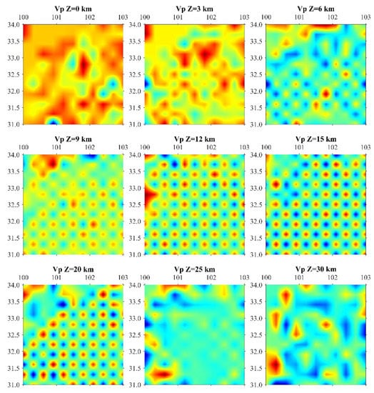
Figure 4.
The accuracy test of inversion in this paper uses the checkerboard test method. This is the checkerboard results of P-wave velocity at different depth levels(0.3° × 0.3°). It can be seen from this figure that VP recovered well in the 6–20 km. There is slight trailing in the 3 and 25 km depth layers. At 0 and 30 km, the smearing is severe, and anomalies in the checkerboard are not expected to recover.
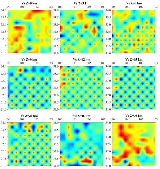
Figure 5.
Checkerboard results of S-wave velocity at different depth levels(0.3° × 0.3°). Similar to the chessboard test result of P-wave, it can be seen from this figure VS recovered well in the 6–20 km. There is also slight trailing in the 3 and 25 km depth layers. At 0 and 30 km, the smearing is severe, and anomalies in the checkerboard are not expected to recover.
4.3. Inversion Results
In our research, we obtained 6,764,713 pairs of P-wave seismic phases and 6,142,190 pairs of S-wave seismic phases after seismic matching using 8649 seismic events after VELEST relocation. After 14 iterations of inversion, we obtained the relocation results (average horizontal error of 183 m and vertical error of 335 m), 3D velocity, and VP/VS wave velocity ratio results for the 7177 seismic events of this Maerkang earthquake sequence.
The time-space distribution of earthquakes can well depict the nature of earthquake-generating fault movement [47,48]. The spatial locations of the three MS 5.0 or higher earthquakes were shown in the precise relocation results: 0:03 MS 5.8 Maerkang earthquake: 32.28° N, 101.81° E, depth 12.3 km; 1:28 MS 6.0 Maerkang earthquake: 32.28° N, 101.83° E, depth 18.8 km; 3:27 MS 5.2 aftershock: 32.26° N 101.86° E, depth 19.45 km. Combined with the relocation epicenter distribution of this earthquake sequence shown in Figure 6, it is evident that the whole sequence tends to migrate southeastward and deeper within 10 h after the earthquake.
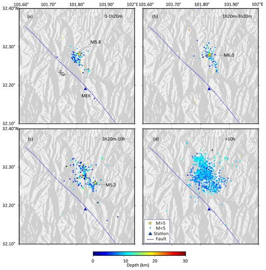
Figure 6.
Time and space distribution of Maerkang aftershock sequence (starting from the occurrence time of MS 5.8 main shock, (a–d)represent the aftershock sequence between 1 h 20 min, 1 h 20 min–3 h 20 min, 3 h 20 min–10 h and 10 h–15 June 2022 respectively).
5. Discussion
In order to discuss the characteristics of crustal velocity structure in the Maerkang area, detailed research has been carried out from one-dimensional velocity to precise seismic location and three-dimensional velocity inversion. The results can provide an important reference for seismic location and analysis of earthquake-generating mechanisms in this area.
From the relocation results, we found that the aftershock sequence of the Maerkang earthquake moved southeastward and deeper underground (Figure 6). According to the analysis of regional tectonic stress research results, this is mainly due to the influence of the enormous stress environment of the block extrusion on the Tibetan Plateau, Like most other earthquakes in the Qinghai Tibet Plateau [49,50]. When the crustal material of the Tibetan Plateau migrated eastward, it was obstructed by the hard Sichuan Basin in the east to generate stress accumulation. When the accumulation reached a certain degree, a large number of earthquakes were induced by fault destabilization [32]. This Maerkang earthquake sequence proves it. In addition, we can find that the aftershock sequence did not occur on the Songgang Fault but on a fault parallel to the Songgang Fault with its north-east direction of about 5 km and a strike of 300–310°, according to the epicenter distribution in Figure 6. Moreover, the distribution of the seismic sequence at depth (Figure 7 and Figure 8) also shows that the seismogenic fault is not the Songgang Fault. Therefore, we speculate that the seismogenic fault of this earthquake may be a secondary fault not mapped in the 5th generation active fault map, with a steeper fault dip and a slight southward dip.
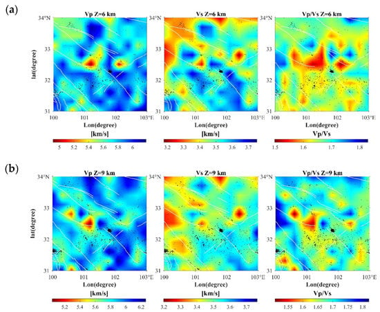
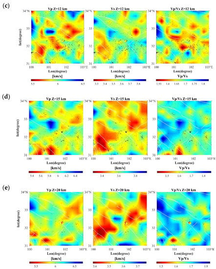
Figure 7.
Imaging results at different depth levels, based on the results of the checkerboard test, here we only show the imaging results in the depth range of 6–20 km. (Black dots in different depth velocity maps represent seismic events after relocation and select earthquakes with half the distance between the upper and lower layers).
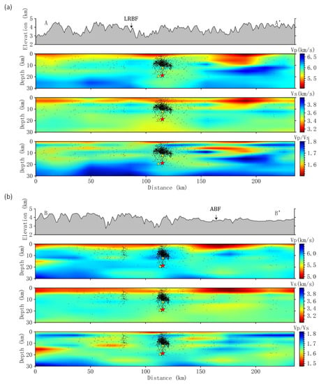
Figure 8.
Three-dimensional velocity and seismic distribution along seismic strike and vertical profile. (a) represents the vertical imaging results of profile AA’, and (b) represents the vertical imaging results of profile BB’. (Black dots are seismic events, and earthquakes within 6 km around the profile line are selected; LRBF: Longriba fault; ABF: Aba fault).
The physical properties of the rock (e.g., density, porosity, fluid content, etc.) influence the seismic velocities (VP and VS), with VP being more positively correlated with the density of the rock. In addition, VP and VS are sensitive to the presence or absence of fluids, so the VP, VS and VP/VS value models all provide information on the crustal composition, including possible partial melting [51]. Based on the results of the checkerboard test, only tomography results within 6–20 km are discussed in this paper. The seismic tomography and location results in this paper (Figure 7 and Figure 8) show that the two events with the largest magnitude in the Maerkang earthquake sequence, MS 5.8 and MS 6.0, occurred on the P and S wave high-velocity and low-velocity intermittent surfaces, where the location of the MS 6.0 earthquake is more to the side of the low-velocity anomaly, and there is a wide range of low-velocity anomalies in the surrounding area. Previous authors analyzed the existence of the low-velocity layer to make the seismogenic layer have a strong seismogenic capacity [52], which may be why the magnitude of the 1:28 MS 6.0 Maerkang earthquake exceeded that of the 0:03 MS 5.8. According to the seismic distribution after relocation (Figure 7 and Figure 8), a large number of earthquakes are distributed along high and low-velocity anomalies or high and low anomalies of VP/VS values, and these areas are usually the intersection of different media, which are more prone to earthquakes, and the distribution direction of earthquakes is consistent with the direction of high-velocity anomalies [53].
The wave velocity in the study area has significant lateral and longitudinal heterogeneity. The vertical distribution of both P and S waves shows significant undulation, which corresponds to the folded deformation of the strata in the study area [54]. In general, the tomography results of the P-wave and S-wave were relatively consistent. High-velocity anomalies dominate P-wave and S-wave at 6–9 km depth and low-velocity anomalies at 12 km–20 km depth. The significant low-velocity zone may be the range of fluid channels in the crust of the Qinghai-Tibet Plateau, and it is assumed that the material nature may be salt-bearing water fluid or local melt in the adjacent Ganzi area [55].
The maximum value of VP/VS calculated by the P-wave to S-wave velocity ratio is 1.86 at a depth of 15 km, and there are two places; one appears on the south side of the Xianshui River Fault in the southwest corner of the study area, and the other is located between the southern margin of the Gande Fault and the eastern end of the Dari Fault. The minimum value is 1.42 at a depth of 15 km, located at the site of the 1973 Luhuo MS 7.6 earthquake. The VP/VS values at 6 and 9 km depths exhibit multiple diamond-shaped masses, which may be related to the gravitational equilibrium in the local mountainous area. The location of the 12 km depth MS 5.8 Maerkang earthquake is surrounded by low VP/VS values and is located at the low-value boundary. The VP/VS values at 15–20 km depth are dominated by high values. Due to the low-speed characteristics of S wave propagation in the liquid, it is generally believed that high VP/VS values are related to saturated fluid [56,57,58,59]. In addition, the S-wave velocity at 15 km depth shows a wide range of S-wave anomalies combined with high VP/VS values that may exist in local melting [60].
The AA’ profile along the earthquake strike shows a clear segmentation of P wave-velocity, S wave-velocity, and VP/VS values at 50 km northwest of the Maerkang earthquake, which is characterized by low-rate subsidence and high-rate uplift, possibly responding to crustal shortening. The vertical profile BB’ shows a steeper dip of the seismic sequence with a slight southward dip. Wang et al. (2003) [45] found a large-scale low-velocity anomaly in the area near Maerkang based on artificial blast profiles. In this paper, BB’ shows similar results, and the profile shows a low-velocity anomaly of about 50 km length along the NE direction after passing through the Aba fault. The vertical distribution of VP/VS values is stepped and more complex, with high VP/VS values gradually extending towards the surface. The velocity anomalies obtained from the inversions described above may be related to the equilibrium response of density anomalies within these mountains.
6. Conclusions
The inversion of underground three-dimensional velocity structure is one of the important means to understand the factors of earthquake occurrence. In this paper, we have used the system operation processing from one-dimensional velocity optimization to three-dimensional velocity inversion to analyze the seismogenic mechanism of the Sichuan Maerkang earthquake swarm in 2022. We optimize the one-dimensional velocity structure using the EA_VELEST method and use the optimized velocity model as the initial velocity model to obtain the three-dimensional fine velocity structure and high-precision inversion and seismic source parameters of the area using the TomoDD method. The following main conclusions were obtained:
(1) We propose a method to quickly obtain the optimal one-dimensional velocity model EA_VELEST, which simplifies the process of one-dimensional velocity inversion and can make VELEST move steadily towards the direction of residual reduction. We believe that combining EA_VELEST and the 3D velocity inversion method is a shortcut to quickly grasp the tectonic environment of earthquake occurrence.
(2) We obtained the precise location result of the Maerkang earthquake case through TomoDD inversion. The distribution of aftershocks after the earthquake relocation along a secondary fault parallel to the Songgang Fault, which may be the seismogenic fault of this earthquake, with a steeper dip, slightly southward, towards 300–310°, and close to the Songgang Fault.
(3) The earthquakes in the study area are mainly concentrated within 5–15 km with a shallow distribution. The spatial and temporal distribution of the aftershock sequence shows that the seismic sequence extends to the southeast and deeper.
(4) The wave velocity in the study area has obvious lateral and vertical heterogeneity, and the S-wave velocity at 15 km depth shows a wide range of S-wave anomalies. Combined with high VP/VS values, it is speculated that local melting may exist. Most of the earthquakes are distributed along high and low-velocity anomalies or high and low anomalies of VP/VS values.
The aftershocks of the Maerkang earthquake sequence are still active, so the calculation results of this paper still need to be improved, but the velocity tomography obtained from this study is still more reliable according to the results of the checkerboard test, and further analysis will be done later with the further accumulation of seismic data. From the research results in this paper, we suggest that we should continue to pay attention to Markang and its surrounding areas and reveal the seismic risk of this area through three-dimensional velocity changes in different time periods.
Author Contributions
Conceptualization, X.Y. and F.L.; methodology, X.Y., F.L. and X.Z.; investigation, F.L., R.C. and H.W.; resources, R.C. and H.W.; software, X.Y., R.C. and X.Z.; data curation, R.C. and X.Z.; supervision, H.W. and F.L.; project administration, F.L. and H.W.; funding acquisition, X.Y. and H.W. All authors have read and agreed to the published version of the manuscript.
Funding
This work is supported by the Basic Research Project of Institute of Earthquake Forecasting, China Earthquake Administration [2021IESLZ4]; The Gansu Earthquake Administration innovation team special fund under grant agreement number [2019TD-01-02]; The National Natural Science Foundation of China under grant agreement number [41601479]; The Gansu Province Science and Technology Program under grant agreement number [21JR7RA795, 21YF5FA031, 22JR5RA822] and the Key Talent Project of Gansu Province under grant agreement number [11276679015] are jointly funded.
Institutional Review Board Statement
Not applicable.
Informed Consent Statement
Not applicable.
Data Availability Statement
Not applicable.
Acknowledgments
We thank Haijiang Zhang of the University of Science and Technology of China for providing the TomoDD program and the seismic phase report information provided by the seismic station networks in Sichuan, Gansu, and Qinghai, and we also use GMT mapping software [61] to make the maps in this paper, which is greatly appreciated. Thanks to the deep learning technology team of the Cross-Innovation Laboratory of East China Normal University for their full support. We also thank the reviewers for their valuable time.
Conflicts of Interest
The funders had no role in the design of the study; in the collection, analyses, or interpretation of data; in the writing of the manuscript, or in the decision to publish the results.
References
- Zhang, H.B.; Tao, Z.G. Evaluating China’s paired-assistance policy (PAP) in response to the Wenchuan earthquake: A sustainability perspective. Sustainability 2018, 10, 3732. [Google Scholar] [CrossRef]
- Mavrodieva, A.V.; Daramita RI, F.; Arsono, A.Y.; Yawen, L.; Shaw, R. Role of civil society in sustainable urban renewal (Machizukuri) after the Kobe Earthquake. Sustainability 2019, 11, 335. [Google Scholar] [CrossRef]
- Fernández, P.; Ceacero-Moreno, M. Urban sustainability and natural hazards management; designs using simulations. Sustainability 2021, 13, 649. [Google Scholar] [CrossRef]
- Guo, L.; Qian, J.; Zhang, S.; Zhou, Y.; Wang, X. Seismicity and velocity structure of the 2020 MS 5.1 Tangshan earthquake. J. Seismol. 2022, 26, 359–371. [Google Scholar] [CrossRef]
- Feng, T.; Zhang, M.; Xu, L.; Wu, J.; Fang, L. Machine learning-based earthquake catalog and tomography characterize the middle-northern section of the Xiaojiang fault zone. Seismol. Soc. Am. 2022, 93, 2484–2497. [Google Scholar] [CrossRef]
- Bannister, S.; Bertrand, E.A.; Heimann, S.; Bourguignon, S.; Asher, C.; Shanks, J.; Harvison, A. Imaging sub-caldera structure with local seismicity, Okataina Volcanic Centre, Taupo Volcanic Zone, using double-difference seismic tomograph. J. Volcanol. Geotherm. Res. 2022, 431, 107653. [Google Scholar] [CrossRef]
- Zhang, Z.; Deng, Y.; Qiu, H.; Peng, Z.; Liu-Zeng, J. High-Resolution Imaging of Fault Zone Structure Along the Creeping Section of the Haiyuan Fault, NE Tibet, from Data Recorded by Dense Seismic Arrays. J. Geophys. Res. Solid Earth 2022, 127, e2022JB024468. [Google Scholar] [CrossRef]
- Sun, Q.; Pei, S.; Cui, Z.; Chen, Y.J.; Liu, Y.; Xue, X.; Li, J.; Li, L.; Zuo, H. Structure-controlled asperities of the 1920 Haiyuan M8. 5 and 1927 Gulang M8 earthquakes, NE Tibet, China, revealed by high-resolution seismic tomography. Sci. Rep. 2021, 11, 1–8. [Google Scholar]
- Jia, J.; Wu, Q.; Wang, F. Three-dimensional crustal P-wave velocity structure in the Yangbi and Eryuan earthquake regions, Yunnan, China. Earthq. Sci. 2021, 34, 358–366. [Google Scholar] [CrossRef]
- Guo, H.; Thurber, C. Temporal Changes in Seismic Velocity and Attenuation at The Geysers Geothermal Field, California, From Double-Difference Tomography. J. Geophys. Res. Solid Earth 2022, 127, e2021JB022938. [Google Scholar] [CrossRef]
- Long, F.; Yi, G.; Wang, S.; Qi, Y.; Zhao, M. Geometry and tectonic deformation of the seismogenic structure for the 8 August 2017 MS 7.0 Jiuzhaigou earthquake sequence, northern Sichuan, China. Earth Planet. Phys. 2019, 3, 253–267. [Google Scholar] [CrossRef]
- Merrill, R.; Bostock, M.G.; Peacock, S.M.; Calvert, A.J.; Christensen, N.I. A double difference tomography study of the Washington forearc: Does Siletzia control crustal seismicity? J. Geophys. Res. Solid Earth 2020, 125, e2020JB019750. [Google Scholar] [CrossRef]
- Menichelli, I.; De Gori, P.; Lucente, F.P.; Improta, L.; Valoroso, L.; Baccheschi, P.; Bagh, S.; Montuori, C.; Chiarabba, C. Minimum 1D VP and VP/VS Models and Hypocentral Determinations in the Central Mediterranean Area. Seismol. Res. Lett. 2022, 93, 2670–2685. [Google Scholar] [CrossRef]
- Zhang, X.; Song, X.; Li, J. A comparative study of seismic tomography models of the Chinese continental lithosphere. Earthq. Sci. 2022, 35, 161–185. [Google Scholar] [CrossRef]
- Ruppert, N.A.; Nayak, A.; Thurber, C.; Richards, C. Aftershock analysis of the 2018 Mw 7.1 Anchorage, Alaska, earthquake: Relocations and regional moment tensors. Seismol. Res. Lett. 2020, 91, 114–125. [Google Scholar] [CrossRef]
- Waldhauser, F.; Ellsworth, W. A Double-Difference earthquake location algorithm: Method and application to the northern Hayward fault, California. Bull. Seismol. Soc. Am. 2000, 90, 1353–1368. [Google Scholar] [CrossRef]
- Matrullo, E.; De Matteis, R.; Satriano, C.; Amoroso, O.; Zollo, A. An improved 1-D seismic velocity model for seismological studies in the Campania–Lucania region (Southern Italy). Geophys. J. Int. 2013, 195, 460–473. [Google Scholar] [CrossRef]
- Kissling, E.; Ellsworth, W.L.; Eberhart-Phillips, D.; Kradolfer, U. Initial reference models in local earthquake tomography. J. Geophys. Res. Solid Earth 1994, 99, 19635–19646. [Google Scholar] [CrossRef]
- Antunes, V.; Planès, T.; Zahradník, J.; Obermann, A.; Alvizuri, C.; Carrier, A.; Lupi, M. Seismotectonics and 1-D velocity model of the Greater Geneva Basin, France–Switzerland. Geophys. J. Int. 2020, 221, 2026–2047. [Google Scholar] [CrossRef]
- Büyükakpınar, P.; Cesca, S.; Hainzl, S.; Jamalreyhani, M.; Heimann, S.; Dahm, T. Reservoir-triggered earthquakes around the Atatürk Dam (Southeastern Turkey). Front. Earth Sci. 2021, 353, 663385. [Google Scholar] [CrossRef]
- Meier, M.; Schlindwein, V.; Scholz, J.R.; Geils, J.; Schmidt-Aursch, M.C.; Krüger, F.; Czuba, W.; Janik, T. Segment-scale seismicity of the ultraslow spreading Knipovich Ridge. Geochem. Geophys. Geosystems 2021, 22, e2020GC009375. [Google Scholar] [CrossRef]
- Zhang, H.J.; Thurber, C.H. Double-difference tomography: The method and its application to the Hayward fault, California. Bull. Seismol. Soc. Am. 2003, 93, 1875–1889. [Google Scholar] [CrossRef]
- Zhang, H.J.; Thurber, C. Development and applications of Double-Difference seismic tomography. Pure Appl. Geophys. 2006, 163, 373–403. [Google Scholar] [CrossRef]
- Liu, J.; Zhang, X.; Wu, W.; Chen, C.; Wang, M.; Yang, M.; Guo, Y.; Wang, J. The Seismo-Ionospheric Disturbances before the 9 June 2022 Maerkang MS 6.0 Earthquake Swarm. Atmosphere 2022, 13, 1745. [Google Scholar] [CrossRef]
- Shao, X.; Xu, C.; Wang, P.; Li, L.; He, X.; Chen, Z.; Huang, Y.; Xu, X. Two public inventories of landslides induced by the 10 June 2022 Maerkang Earthquake swarm, China and ancient landslides in the affected area. Nat. Hazards Res. 2022. [Google Scholar] [CrossRef]
- Kulhánek, O. The Structure and Interpretation of Seismograms; Academic Press: Cambridge, MA, USA, 2002; pp. 333–348. [Google Scholar]
- Zhu, H.; Long, F. Application of single station amplitude—Ratio method to the judgment of Maerkang MS 4.7earthquake sequence. Seismol. Geomagn. Obs. Res. 2005, 4, 29–35. (In Chinese) [Google Scholar]
- Zhang, Y.J.; Peng, L.G.; Cheng, W.Z. Study on Source Parameters of the Maerkang Earthquake Sequence. Earthq. Res. China 2006, 85–93. (In Chinese) [Google Scholar]
- Zhu, Y.Q.; Wen, X.Z.; Sun, H.P.; Guo, S.S.; Zhao, Y.F. Gravity changes before the Lushan, Sichuan, MS 7. 0 Earthquake of 2013. Chin. J. Geophys. 2013, 56, 1887–1894. (In Chinese) [Google Scholar] [CrossRef]
- Yin, X.; Jiang, C.; Cai, R.; Guo, X.; Jiang, C.; Wang, Z.; Zou, X. Study of crustal tomography and precise earthquake location in Yangbi area, Yunnan province. Seismol. Egology 2021, 43, 864–880. (In Chinese) [Google Scholar]
- Su, J.; Liu, M.; Zhang, Y.; Wang, W.; Li, H.; Yang, J.; Li, X.; Zhang, M. High resolution earthquake catalog building for the 21 May 2021 Yangbi, Yunnan, MS 6.4 earthquake sequence using deep-learning phase picker. Chin. J. Geophys. 2021, 64, 2647–2656. (In Chinese) [Google Scholar] [CrossRef]
- Xu, X.-W.; Zhang, P.-Z.; Wen, X.-Z.; Qin, Z.-L.; Chen, G.-H.; Zhu, A.-L. Features of active tectonics and recurrence behaviors of strong earthquakes in the western Sichuan province and its adjacent regions. Seismol. Geol. 2005, 27, 446–461. (In Chinese) [Google Scholar]
- Cui, B. Geological Tectonic Features and Activity Analysis of Aba Fault in West Sichuan. Master’s Thesis, Chengdu University of Technology, Chengdu, China, 2020. (In Chinese). [Google Scholar] [CrossRef]
- Ren, J.; Xu, X.; Yeats, R.S.; Zhang, S. Latest Quaternary paleoseismology and slip rates of the Longriba fault zone, eastern Tibet: Implications for fault behavior and strain partitioning. Tectonics 2013, 32, 216–238. [Google Scholar] [CrossRef]
- Sun, D.; Wang, D.; Wu, D.; Zhao, D.; Chen, H. Activity and effect of main faults in near field of Bala Hydropower station in Maerkang. J. Eng. Geol. 2003, 18, 940–949. (In Chinese) [Google Scholar]
- Liu, W.L. Regional Crustal Stability of the Jinchuan Hydropower Station Region on the Dadu River. Master’s Thesis, Chengdu University of Technology, Chengdu, China, 2006. (In Chinese). [Google Scholar]
- Zuo, K.Z.; Chen, J.F. 3D body-wave velocity structure of crust and relocation of earthquakes in the Menyuan area. Chin. J. Geophys. 2018, 61, 2788–2801. (In Chinese) [Google Scholar]
- Li, S.H.; Wang, Y.B.; Liang, Z.B.; He, S.L.; Zeng, W.H. Crustal structure in southeastern Gansu from regional seismic waveform inversion. Chin. J. Geophys. 2012, 55, 1186–1197. (In Chinese) [Google Scholar] [CrossRef]
- Yin, X.; Yang, L.; Chen, J.; Wang, Z.; Gao, Y. Study on the One Dimensional Velocity Model in Gansu Area. China Earthq. Eng. J. 2017, 39, 154–159. (In Chinese) [Google Scholar]
- Cai, S.Z.; Yang, M.; Lei, Y.J. Numerical Methods, 2nd ed.; National Defense Industry Press: Beijing, China, 2016. (In Chinese) [Google Scholar]
- Hansen, P.C.; Oleary, D.P. The use of the L-curve in the regularization of discrete ill-posed problems. SIAM J. Sci. Comput. 1993, 14, 1487–1503. [Google Scholar] [CrossRef]
- Yin, X.; Liu, F.; Cai, R.; Yang, X.; Zhang, X.; Ning, M.; Shen, S. Research on Seismic Signal Analysis Based on Machine Learning. Appl. Sci. 2022, 12, 8389. [Google Scholar] [CrossRef]
- Liu, F.; Wang, H.; Zhang, J.; Fu, Z.; Zhou, A.; Qi, J.; Li, Z. EvoGAN: An evolutionary computation assisted GAN. Neurocomputing 2022, 469, 81–90. [Google Scholar] [CrossRef]
- Lei, X.; Huang, D.; Su, J.; Jiang, G.; Wang, X.; Wang, H.; Guo, X.; Fu, H. Fault reactivation and earthquakes with magnitudes of up to MW 4.7 induced by shale-gas hydraulic fracturing in Sichuan Basin, China. Sci. Rep. 2017, 7, 1–12. [Google Scholar]
- Wang, C.Y.; Han, W.B.; Wu, J.P.; Lou, H.; Bai, Z.M. Crustal structure beneath the Songpan—Garze orogenic belt. Acta Seismol. Sin. 2003, 16, 229–241+342. (In Chinese) [Google Scholar] [CrossRef]
- Du, M.F. Location of Small Seismic Essence in Aba Area and Its Active Structural Significance. Master’s Thesis, Chengdu University of Technology, Chengdu, China, 2020. (In Chinese). [Google Scholar]
- McGregor, R.F.D.; Illsley-Kemp, F.; Townend, J. The 2001 Taupō Fault Belt seismicity as evidence of magma-tectonic interaction at Taupō volcano. Geochem. Geophys. Geosystems 2022, 23, e2022GC010625. [Google Scholar] [CrossRef]
- Zhou, Y.; Xu, L.; Wu, J.; Li, C.; Fang, L.; Pan, Z. Seismicity of the repeating earthquake clusters in the northern Xiaojiang fault zone and its implications. Front. Earth Sci. 2022, 10, 917635. [Google Scholar] [CrossRef]
- Gao, Z.; Li, Y.; Shan, X.; Zhu, C. Earthquake magnitude estimation from high-rate GNSS data: A case study of the 2021 Mw 7.3 Maduo earthquake. Remote Sens. 2021, 13, 4478. [Google Scholar] [CrossRef]
- Peng, C.; Jiang, P.; Ma, Q.; Su, J.; Cai, Y.; Zheng, Y. Chinese Nationwide Earthquake Early Warning System and Its Performance in the 2022 Lushan M6. 1 Earthquake. Remote Sens. 2022, 14, 4269. [Google Scholar] [CrossRef]
- Lin, G.; Huerfano, V.A.; Fan, W. Crustal Architecture of Puerto Rico Using Body-Wave Seismic Tomography and High-Resolution Earthquake Relocation. Seismol. Soc. Am. 2022, 93, 555–566. [Google Scholar] [CrossRef]
- Wang, X.-N.; Deng, Z.-H.; Ye, X.-W.; Wang, L.-W. The study of crustal velocity structure and seismicity in Yangjiang area of Guangdong province. Seismol. Geol. 2020, 42, 1153–1171. (In Chinese) [Google Scholar]
- Zhang, Y.; Wang, W.; Yang, W.; Liu, M.; Su, J.; Li, X.; Yang, J. Three-dimensional velocity structure around the focal area of the 2021 MS 6.4 YangBi earthquake. Earthq. Sci. 2021, 34, 399–412. [Google Scholar] [CrossRef]
- Zhang, X.Y.; Gao, R.; Bai, Z.M.; Xu, T.; Li, Q.S. Crustal structure beneath the Longmenshan area in eastern Tibet:new constrains from reprocessing wide-angle seismic data of the Aba-Longmenshan-Suining profile. Chin. J. Geophys. 2017, 60, 2200–2212. (In Chinese) [Google Scholar] [CrossRef]
- Liu, Z.Q. Study on Electrical Structure in the Southern and Surrounding Areas of Songpan-Ganzi Block. Master’s Thesis, China University of Geosciences, Beijing, China, 2019. [Google Scholar]
- Wang, X.Q.; Schubnel, A.; Fortin, J.; David, E.C.; Guéguen, Y.; Ge, H.K. High Vp/Vs ratio: Saturated cracks or anisotropy effects? Geophys. Res. Lett. 2012, 39, 11. [Google Scholar] [CrossRef]
- Hamada, G.M. Reservoir fluids identification using Vp/Vs ratio? Oil Gas Sci. Technol. 2004, 59, 649–654. [Google Scholar] [CrossRef]
- Brantut, N.; David, E.C. Influence of fluids on VP/VS ratio: Increase or decrease? Geophys. J. Int. 2019, 216, 2037–2043. [Google Scholar] [CrossRef]
- Ding, P.; Wang, D.; Di, G.; Li, X. Investigation of the effects of fracture orientation and saturation on the Vp/Vs ratio and their implications. Rock Mech. Rock Eng. 2019, 52, 3293–3304. [Google Scholar] [CrossRef]
- Ding, Y.Y.; Di, X.L.; Yuan, Z.X.; Xue, G.Y. Three-dimensional shear wave velocity structure and distribution image of VP/VS beneath the Weihe Fault depression. Chin. J. Geophys. 2000, 43, 194–202. (In Chinese) [Google Scholar] [CrossRef]
- Wessel, P.; Luis, J.F.; Uieda, L.; Scharroo, R.; Wobbe, F.; Smith, W.H.F.; Tian, D. The generic mapping tools version 6. Geochem. Geophys. Geosystems 2019, 20, 5556–5564. [Google Scholar] [CrossRef]
Publisher’s Note: MDPI stays neutral with regard to jurisdictional claims in published maps and institutional affiliations. |
© 2022 by the authors. Licensee MDPI, Basel, Switzerland. This article is an open access article distributed under the terms and conditions of the Creative Commons Attribution (CC BY) license (https://creativecommons.org/licenses/by/4.0/).