
Predicting Effluent Quality in Full-Scale Wastewater Treatment Plants Using Shallow and Deep Artificial Neural Networks


Abstract
1. Introduction
2. Theoretical Background
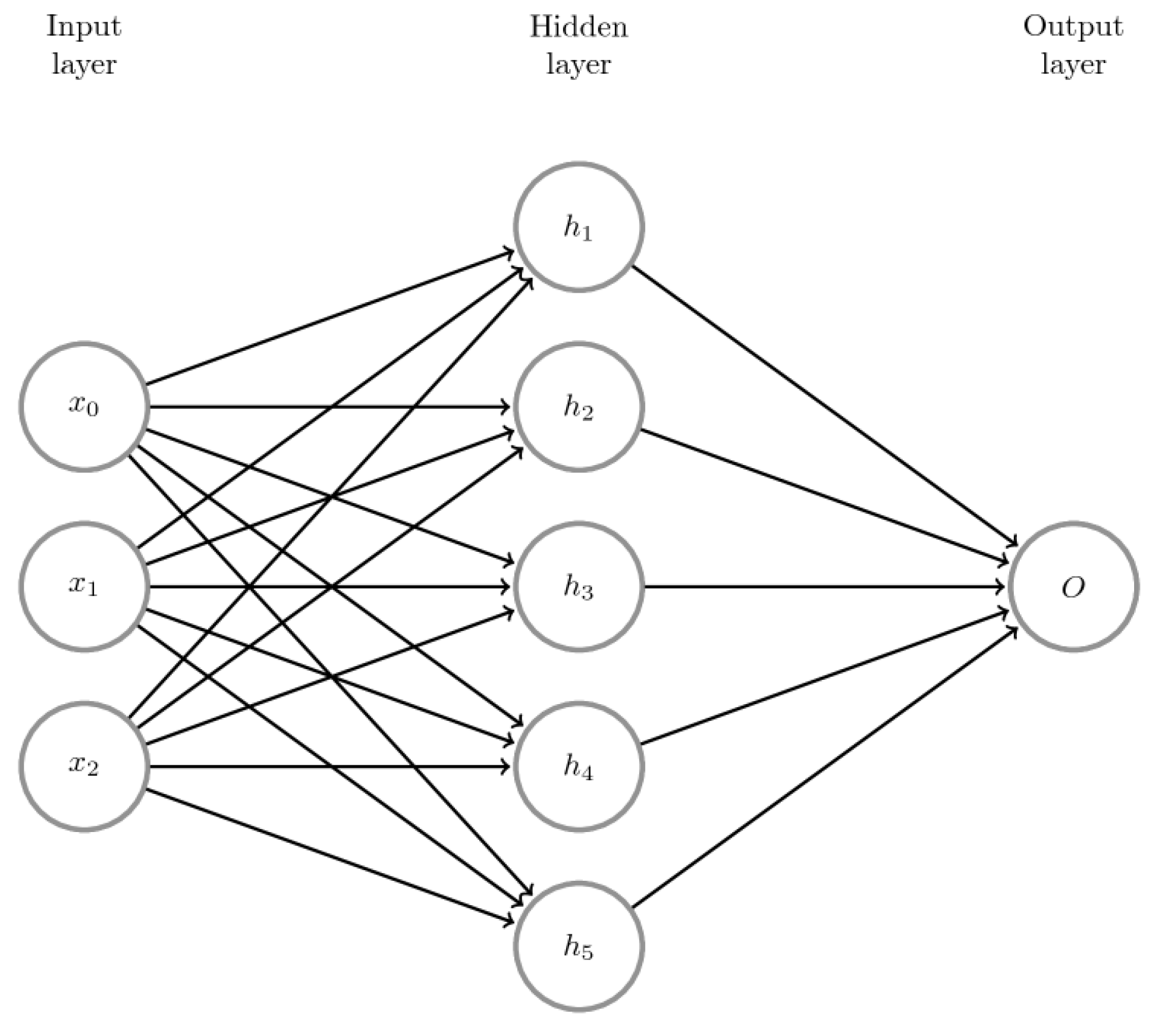
2.1. Artificial Neural Networks Theory
2.2. Deep Neural Networks DNN
3. Materials and Methods
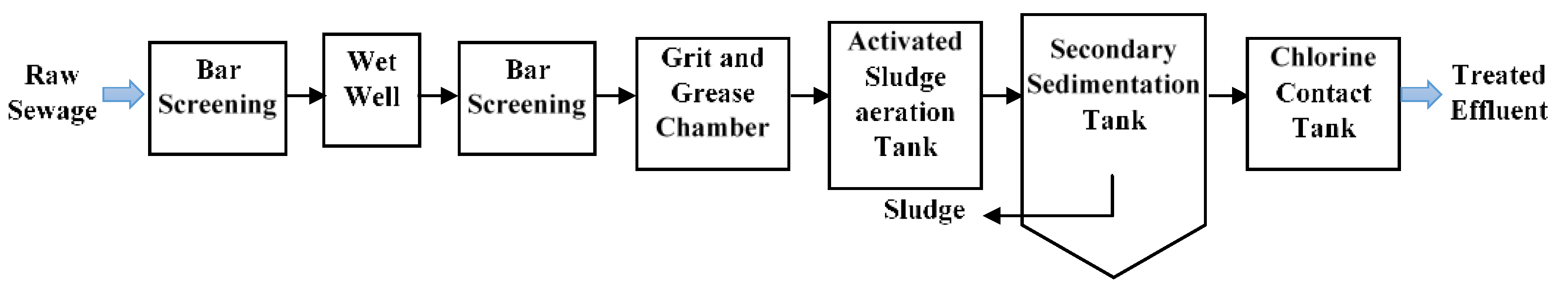
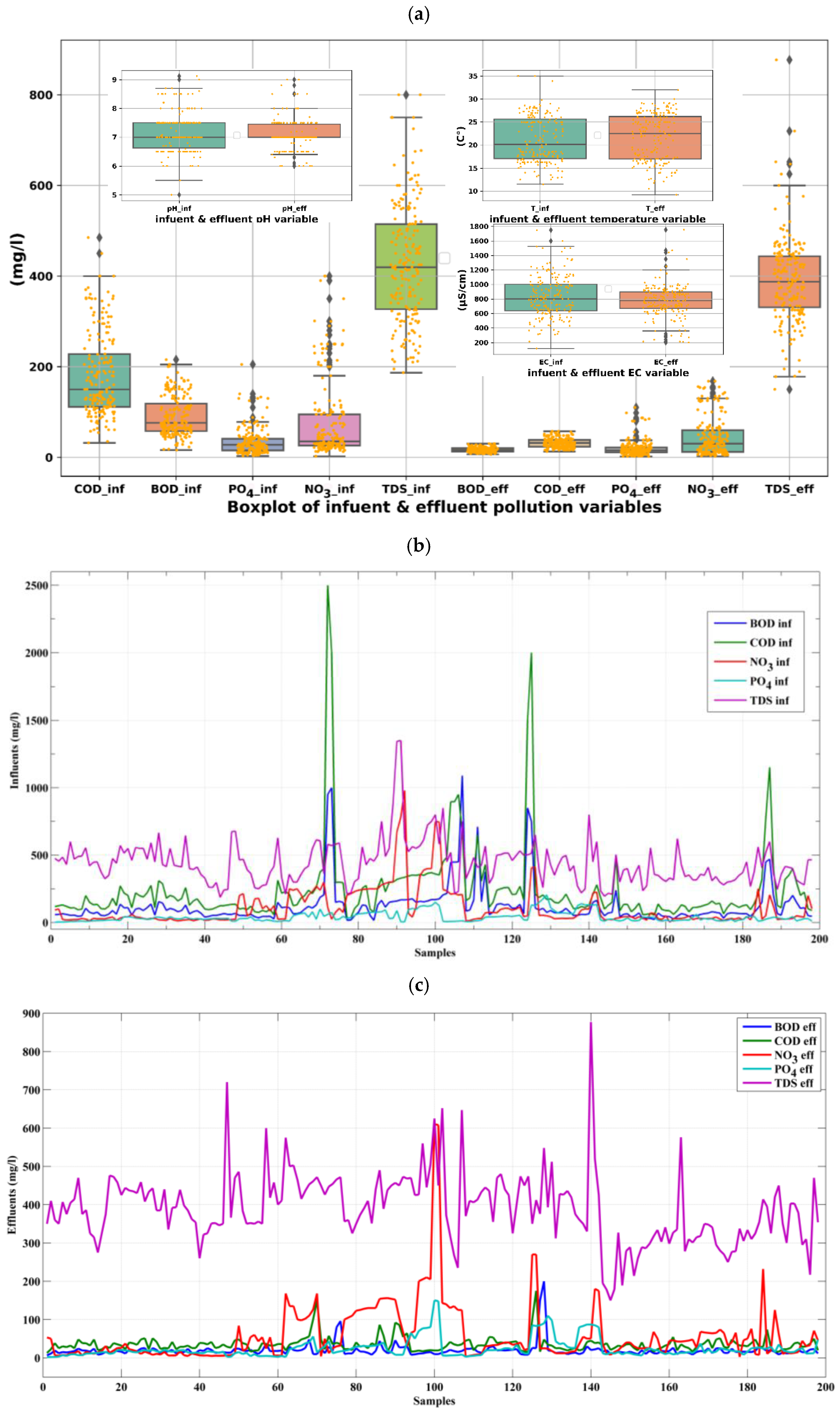
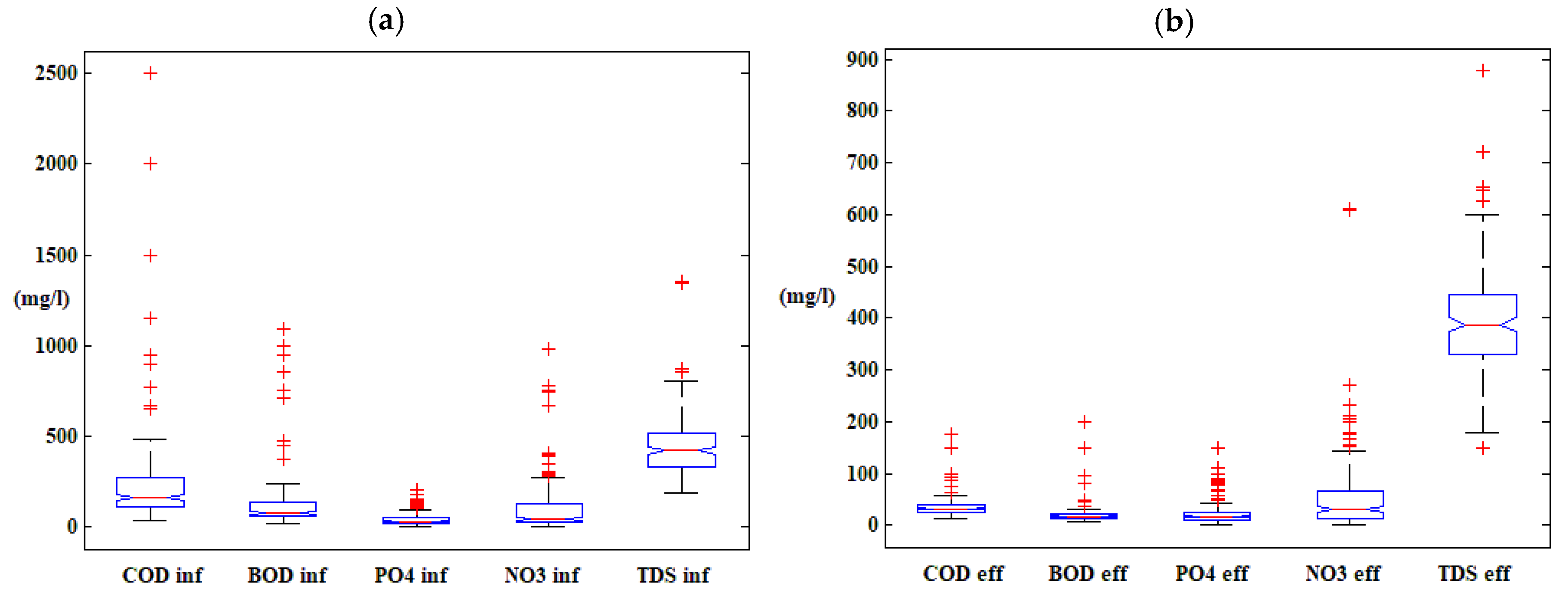
3.1. Plant Description and Data Used
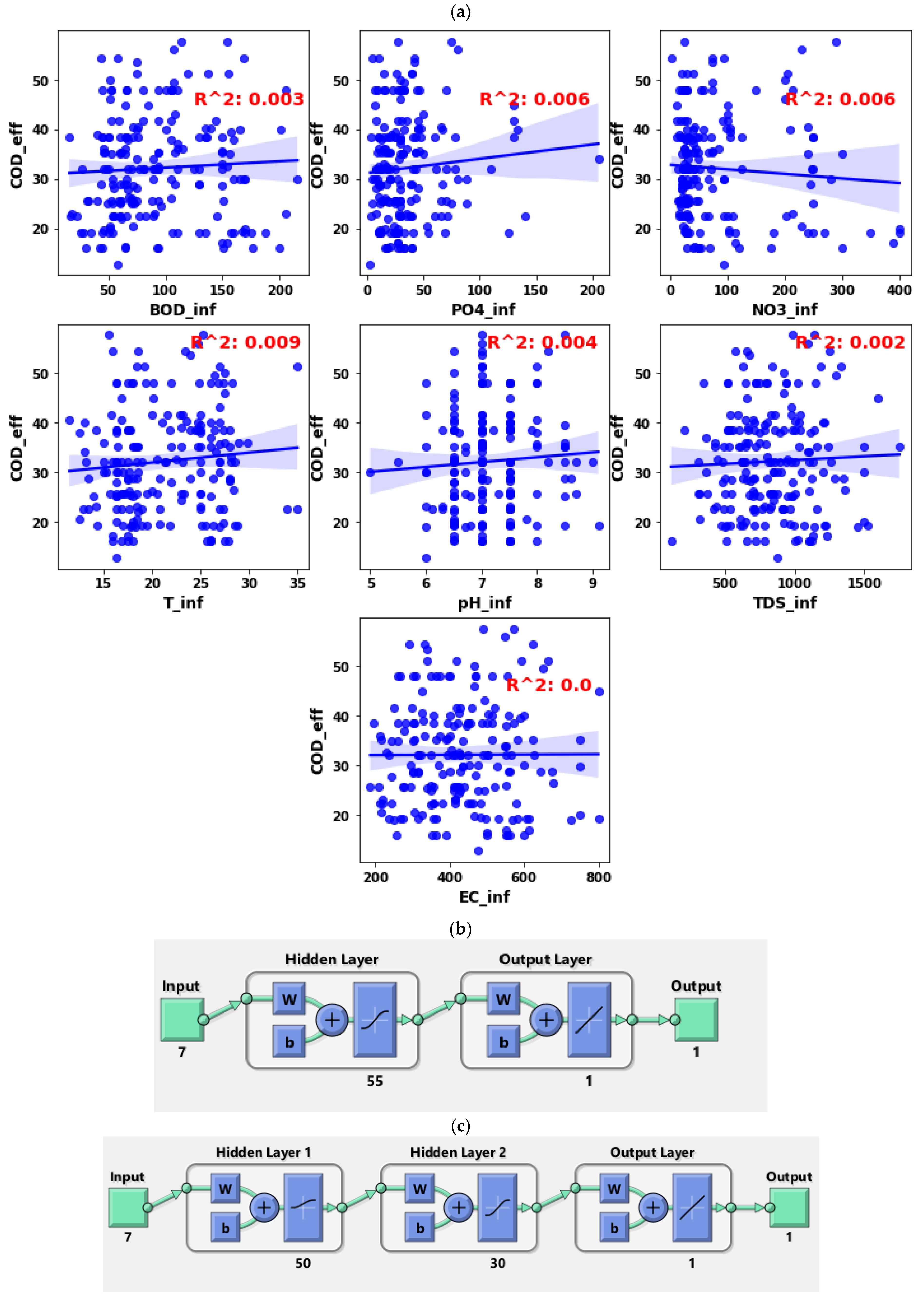
3.2. Models Development
4. Results and Discussion
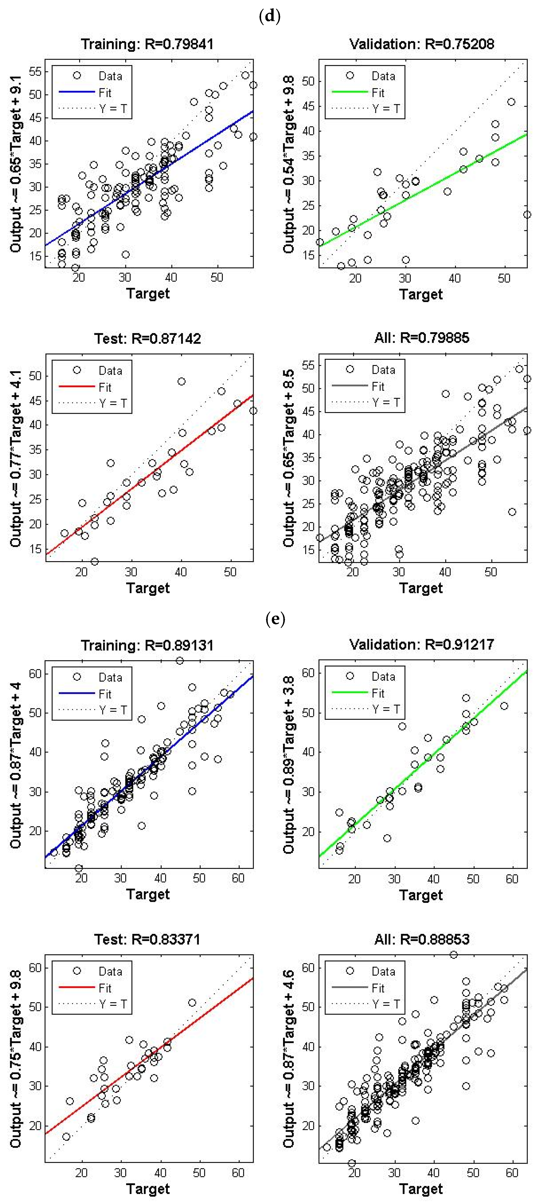
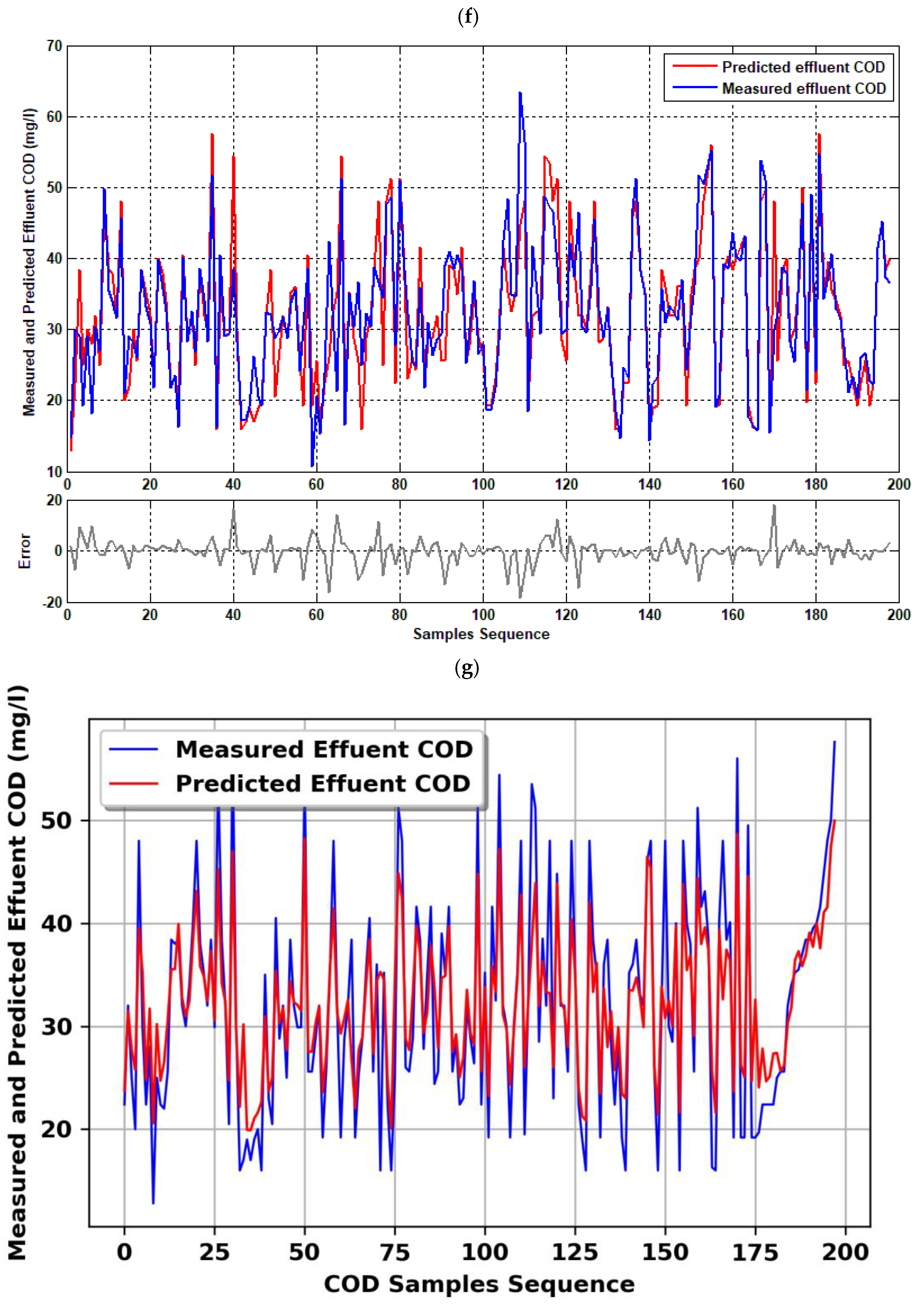
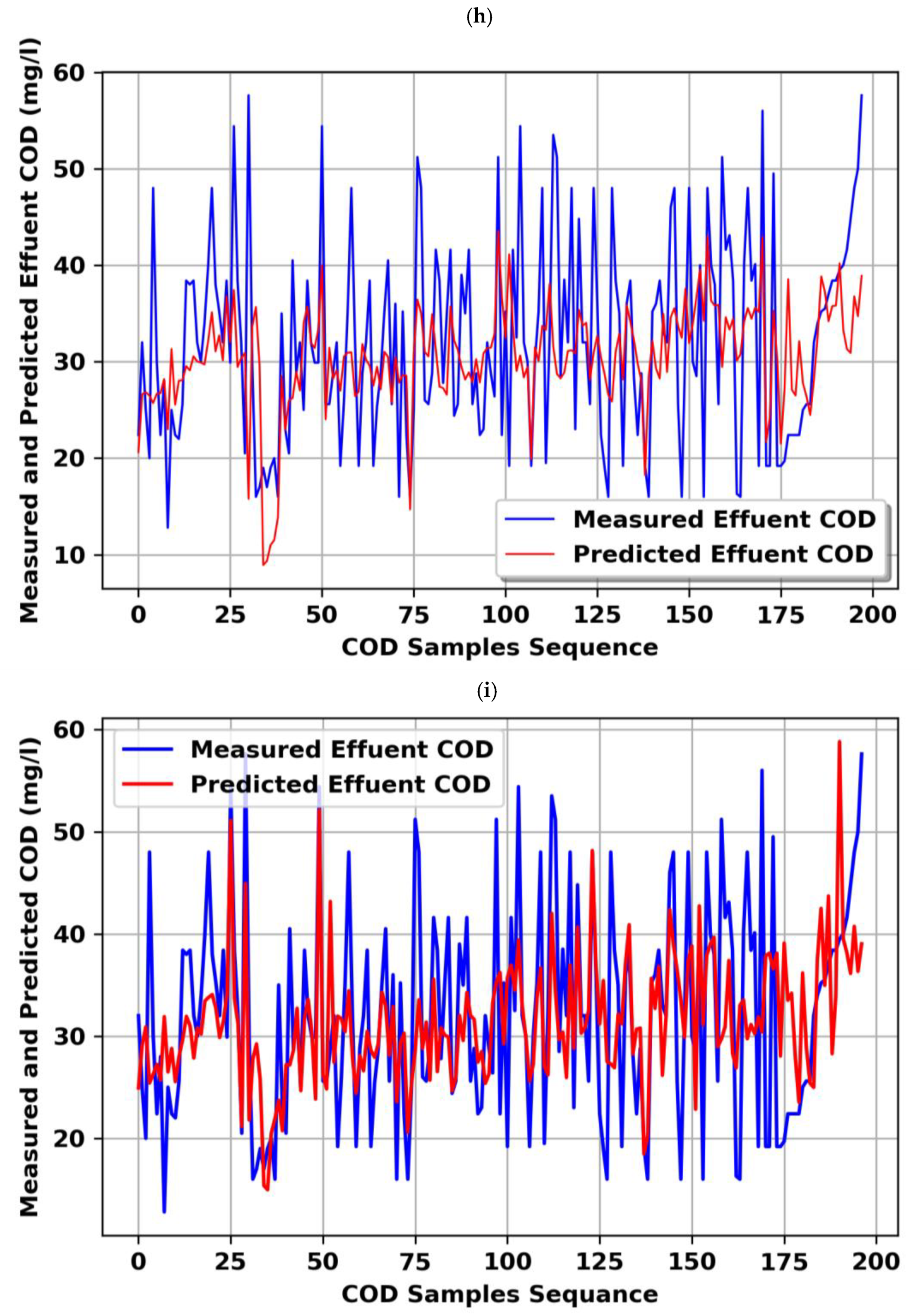
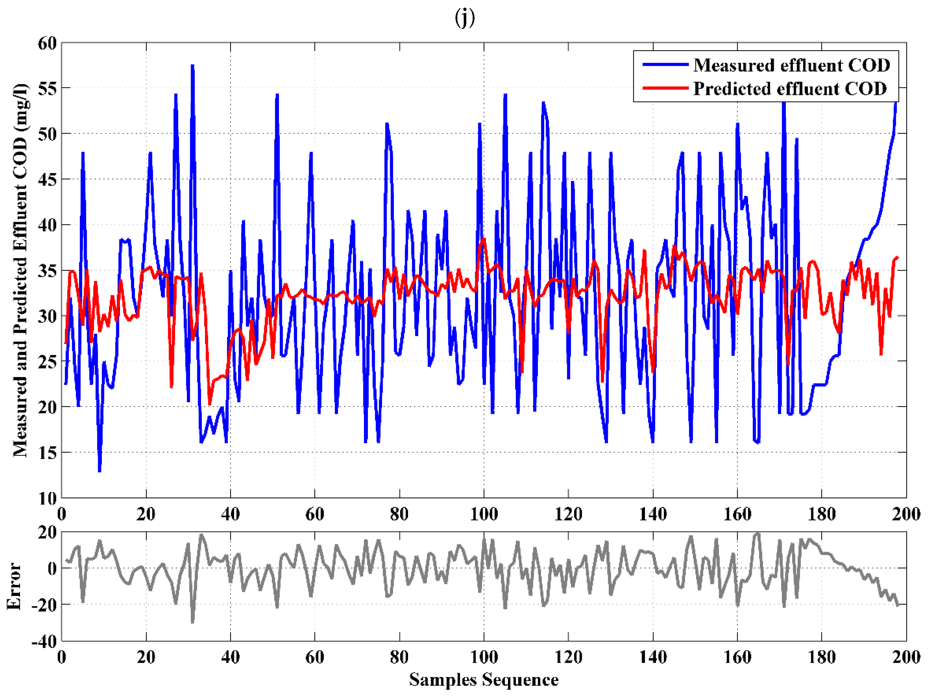
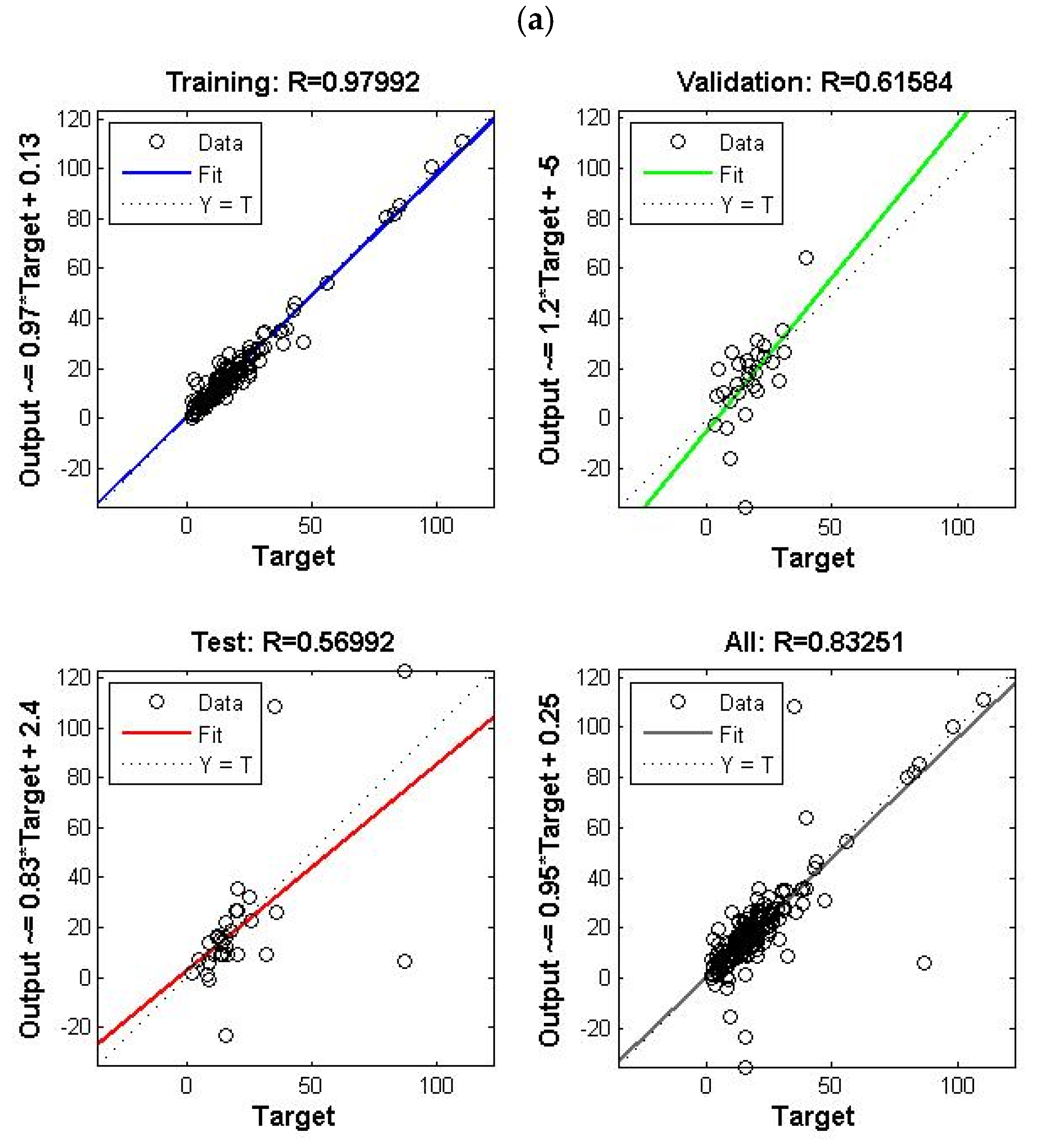
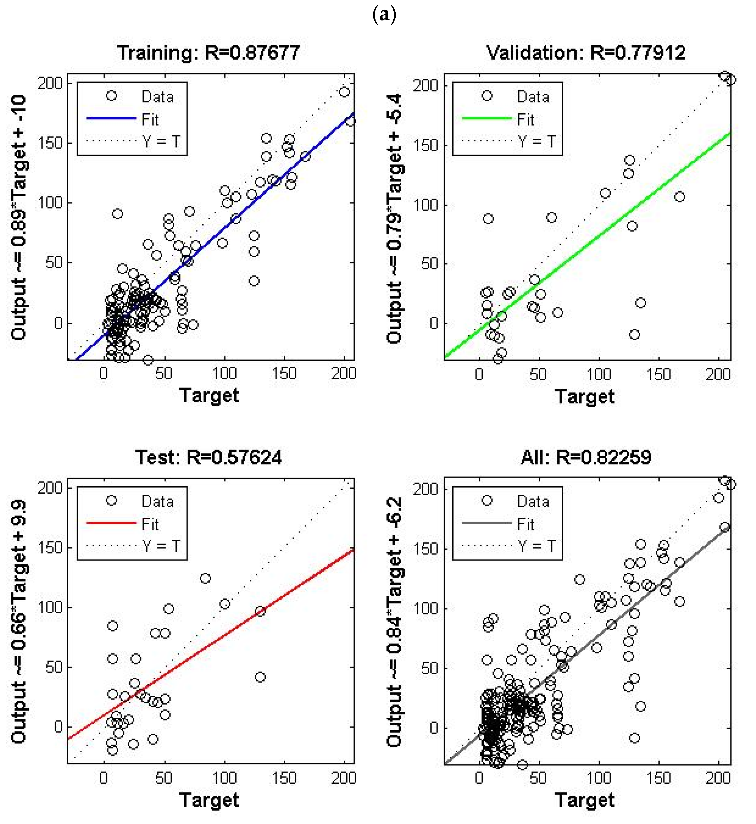
4.1. Single Model (COD Effluent)
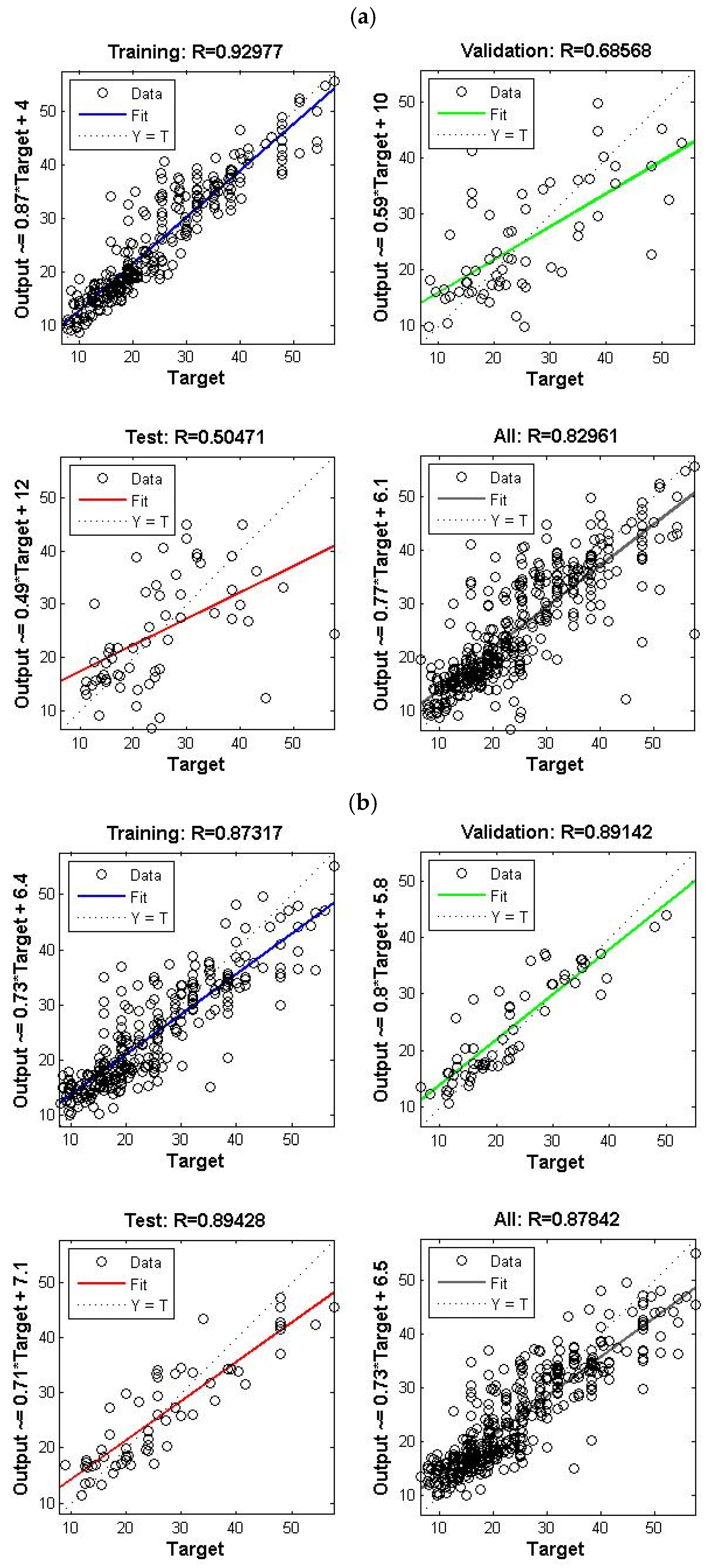
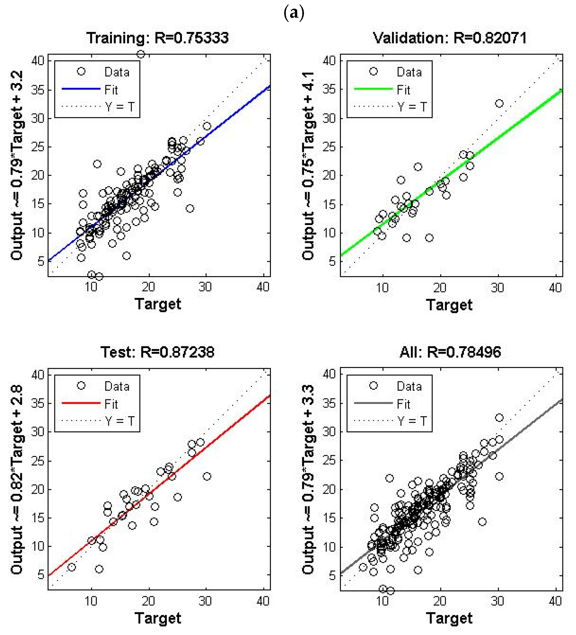
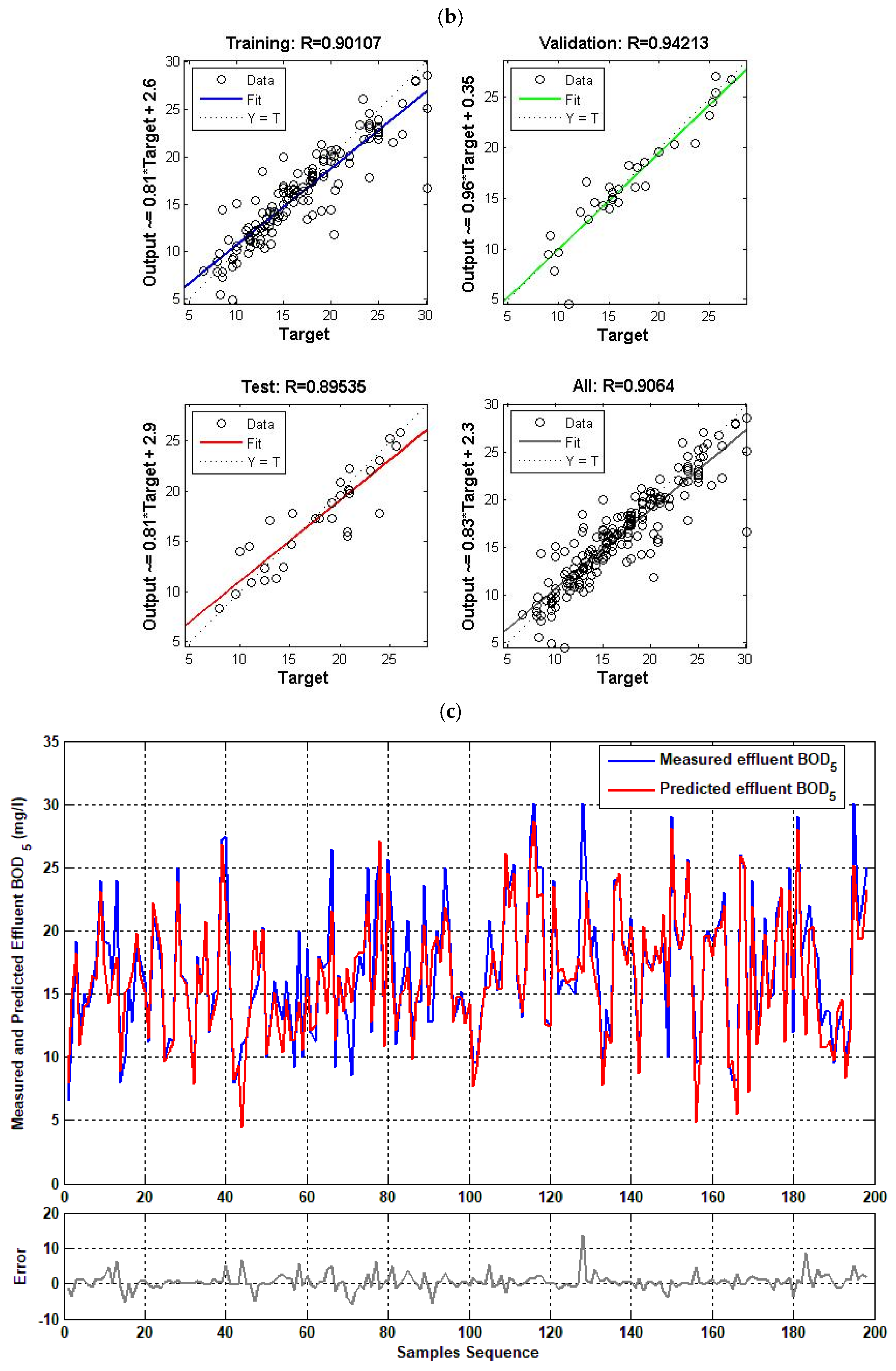
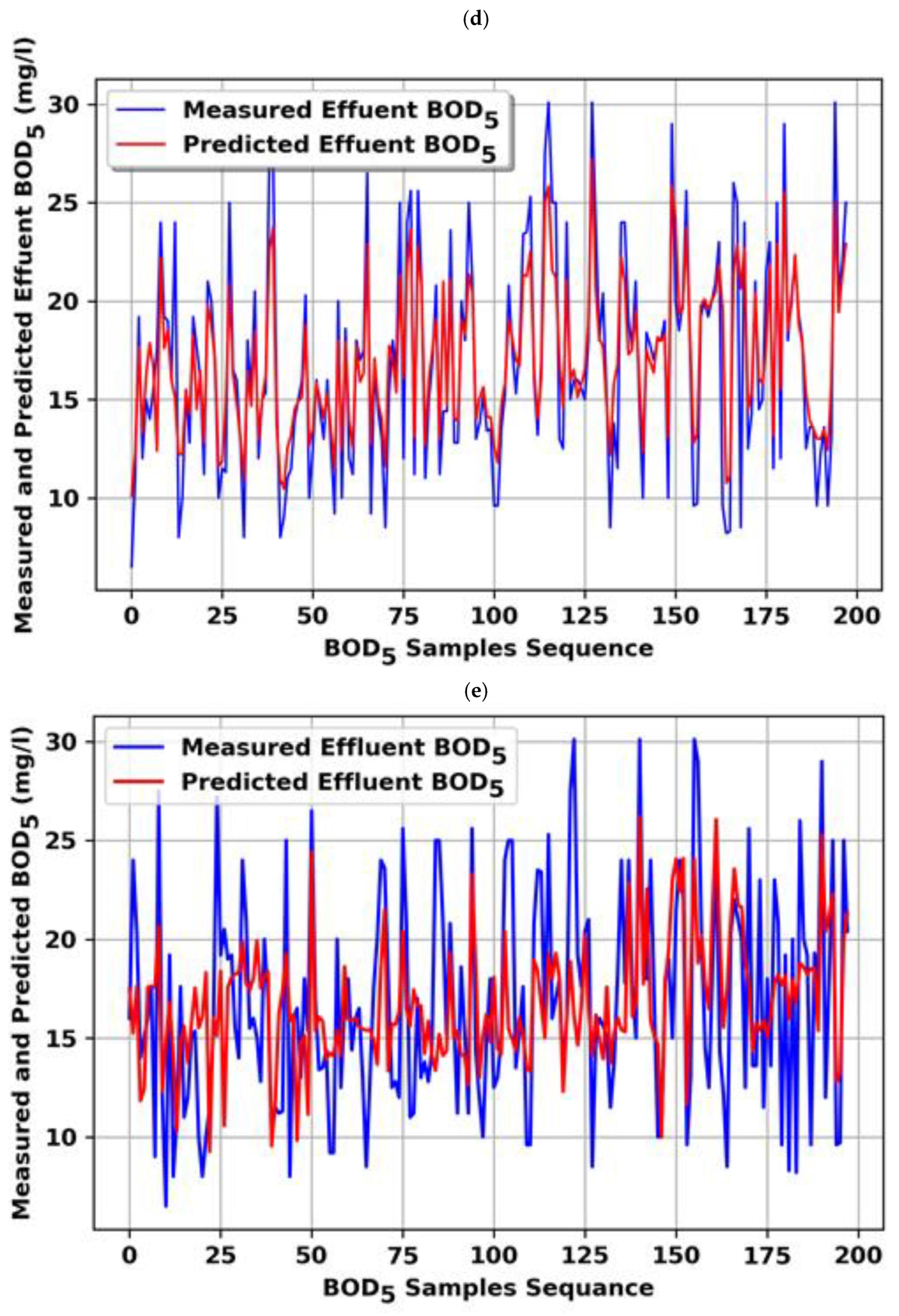
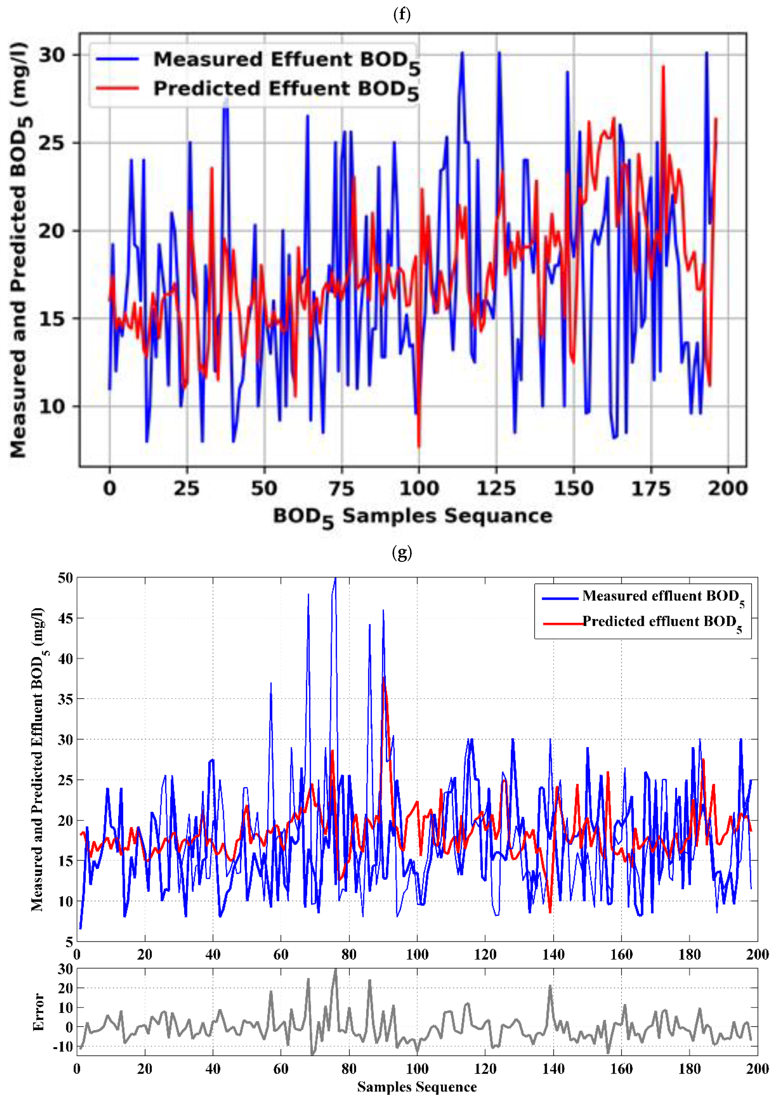
4.2. Single Model (BOD5 Effluent)
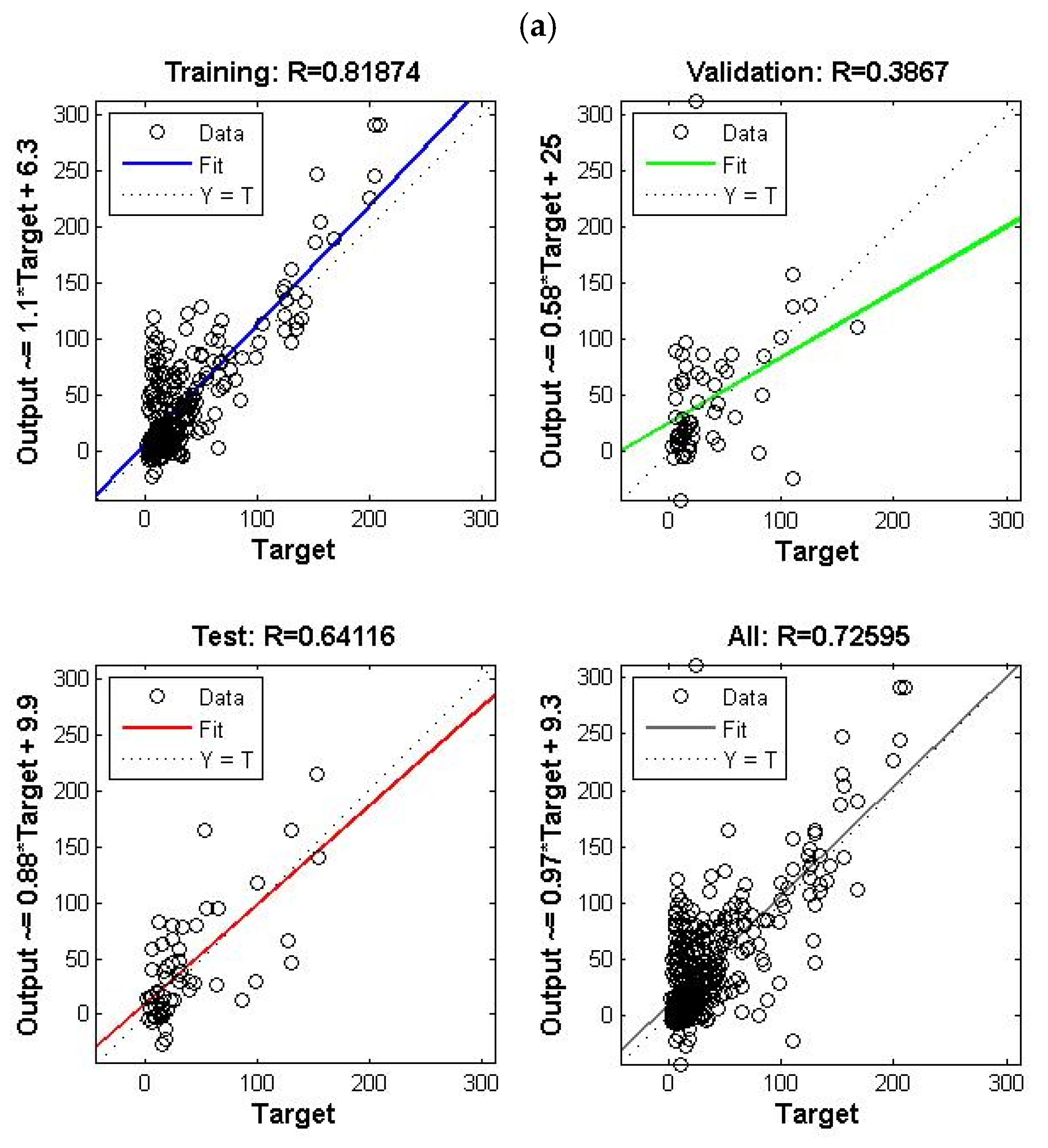
4.3. Single Model ( Effluent)
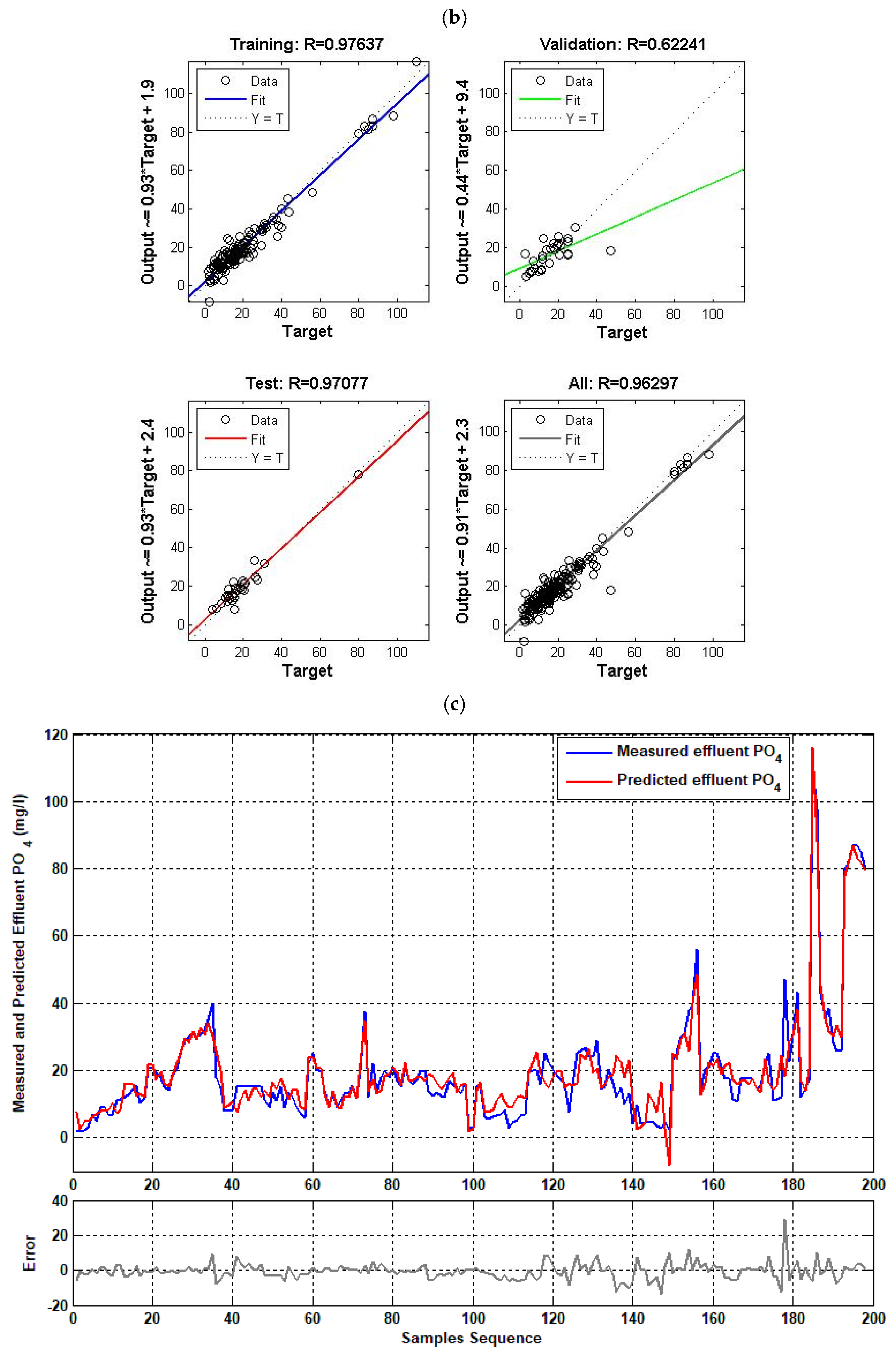
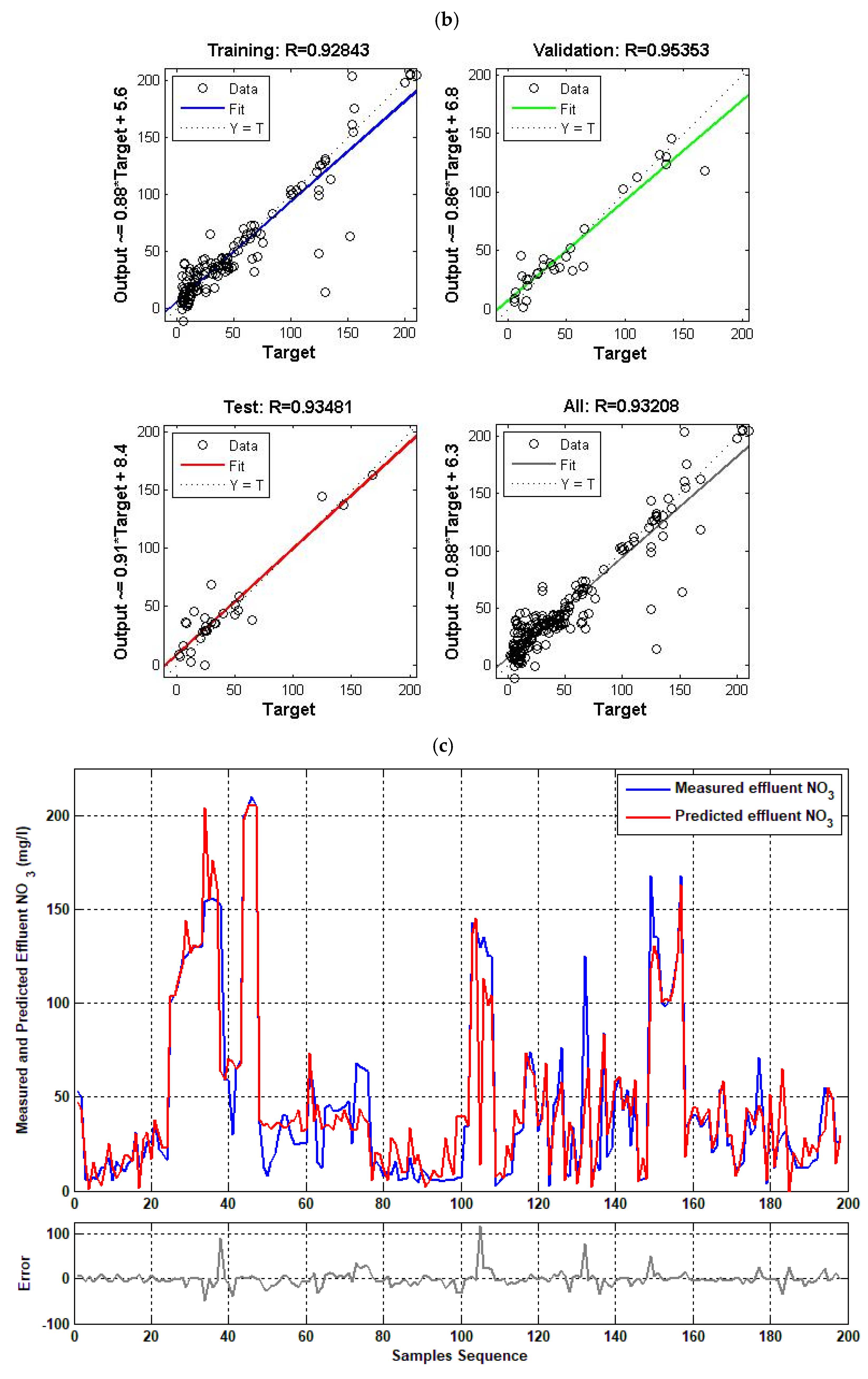
4.4. Single Model ( Effluent)
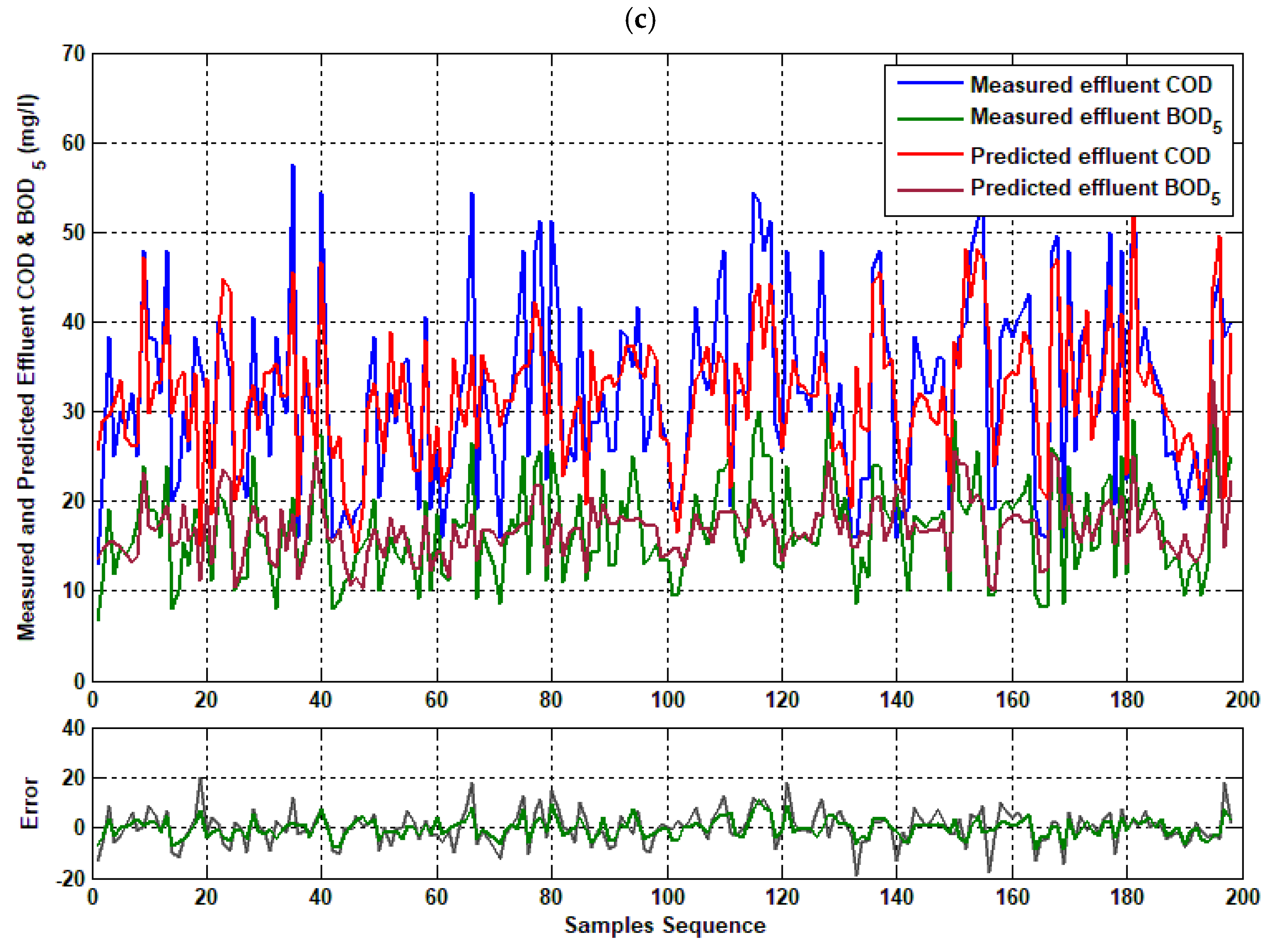
4.5. Ensemble Model (COD and BOD5 Effluent)
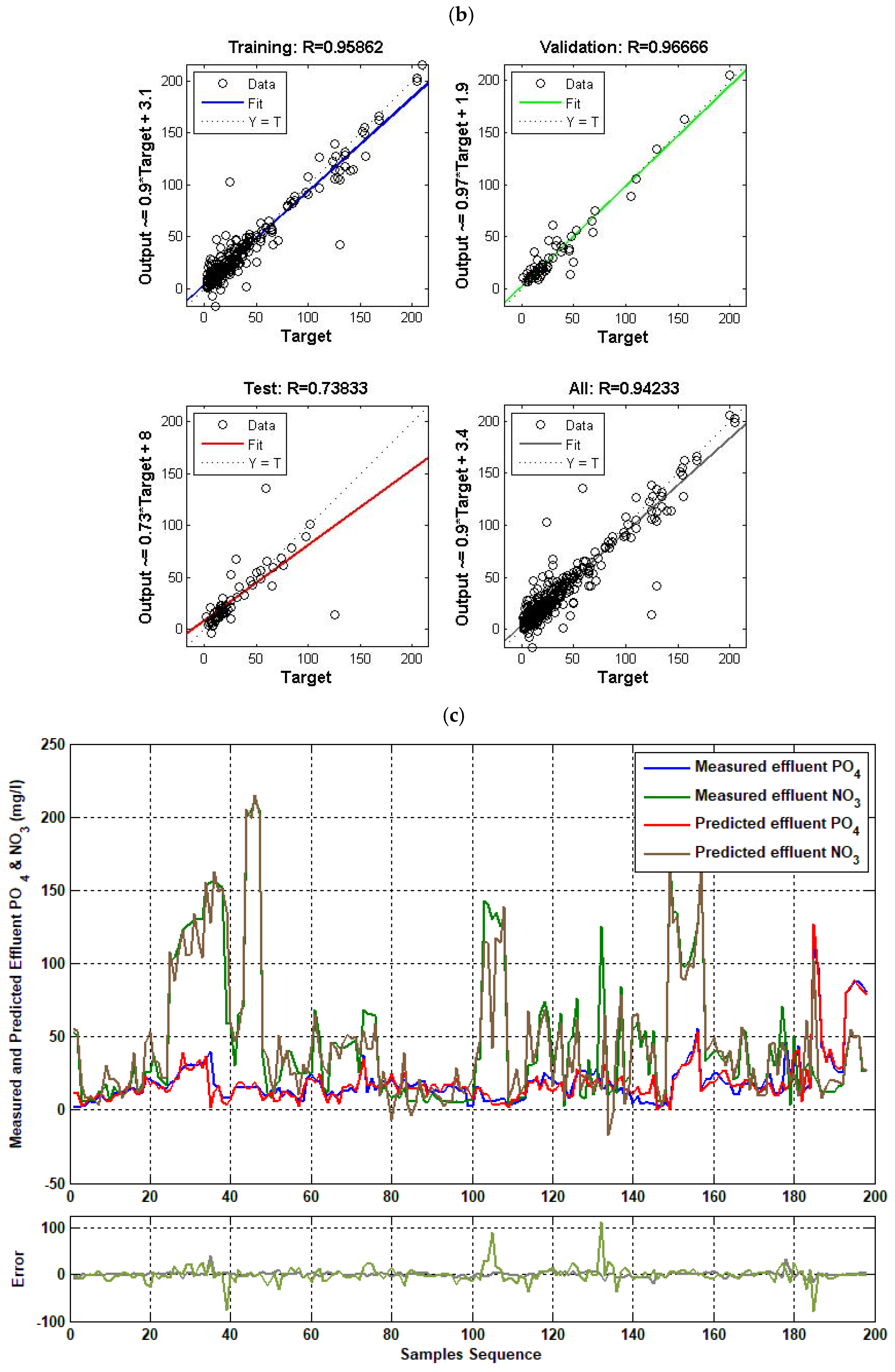
4.6. Ensemble Model ( and Effluent)
4.7. Ensemble Model (COD, BOD5, and Effluent)
5. Conclusions
Author Contributions
Funding
Data Availability Statement
Conflicts of Interest
Appendix A


| Model No. | Model Input Variables | Model Output Variable(S) | Training (Correlation Coefficient) | Validation (Correlation Coefficient) | Testing (Correlation Coefficient) | All Data (Correlation Coefficient) | No. Neurons in Hidden Layers | MSE |
|---|---|---|---|---|---|---|---|---|
| M6-S1 | Tinf, pHinf, ECinf, TDSinf | BOD5eff | 0.515 | 0.774 | 0.564 | 0.541 | 67 | 13.964 |
| M6-S2 | 0.685 | 0.361 | 0.825 | 0.681 | 40–60 | 18.28 | ||
| M7-S1 | Tinf, pHinf, ECinf, TDSinf, inf | BOD5eff | 0.69 | 0.69 | 0.624 | 0.68 | 65 | 10.926 |
| M7-S2 | 0.675 | 0.520 | 0.820 | 0.678 | 30–55 | 18.51 | ||
| M8-S1 | Tinf, pHinf, ECinf, TDSinf, inf, inf | BOD5eff | 0.534 | 0.596 | 0.687 | 0.557 | 65 | 19.223 |
| M8-S2 | 0.704 | 0.648 | 0.825 | 0.715 | 40–60 | 11.10 | ||
| M9-S1 | Tinf, pHinf, ECinf, TDSinf, inf, inf, BOD5inf | BOD5eff | 0.753 | 0.82 | 0.87 | 0.78 | 55 | 10.09 |
| M9-S2 | 0.901 | 0.942 | 0.895 | 0.906 | 30–50 | 2.14 | ||
| M10-S1 | Tinf, pHinf, ECinf, TDSinf, inf, inf, BOD5inf, CODinf | BOD5eff | 0.674 | 0.775 | 0.51 | 0.651 | 60 | 20.224 |
| M10-S2 | 0.890 | 0.935 | 0.898 | 0.898 | 30–50 | 6.55 |


| Model No. | Network Input | Network Output | Training (Correlation Coefficient) | Validation (Correlation Coefficient) | Testing (Correlation Coefficient) | All Data (Correlation Coefficient) | No. Neurons in Hidden Layers | MSE |
|---|---|---|---|---|---|---|---|---|
| M16-S1 | Tinf, pHinf, ECinf, TDSinf | 0.606 | 0.273 | 0.245 | 0.489 | 67 | 4135.91 | |
| M16-S2 | 0.83 | 0.485 | 0.209 | 0.607 | 40–60 | 1915 | ||
| M17-S1 | in | 0.907 | 0.448 | 0.505 | 0.715 | 65 | 5015.33 | |
| M17-S2 | 0.901 | 0.988 | 0.809 | 0.912 | 30–55 | 223.42 | ||
| M18-S1 | inf | 0.972 | 0.598 | 0.661 | 0.789 | 65 | 2054.71 | |
| M18-S2 | 0.90 | 0.975 | 0.864 | 0.909 | 40–60 | 188.87 | ||
| M19-S1 | inf, BOD5inf | 0.969 | 0.698 | 0.581 | 0.793 | 55 | 2520.53 | |
| M19-S2 | 0.905 | 0.844 | 0.914 | 0.9 | 30–50 | 406.11 | ||
| M20-S1 | inf, BOD5inf, CODinf | 0.876 | 0.779 | 0.576 | 0.822 | 60 | 2038.57 | |
| M20-S2 | 0.928 | 0.953 | 0.934 | 0.932 | 30–50 | 65.94 |


| Model No. | Network Input | Network Output | Training (Correlation Coefficient) | Validation (Correlation Coefficient) | Testing (Correlation Coefficient) | All Data (Correlation Coefficient) | No. Neurons in Hidden Layers | MSE |
|---|---|---|---|---|---|---|---|---|
| M31-S1 | Tin, pHin, ECin, TDSin | CODeff & BOD5eff & & | 0.872 | 0.30 | 0.62 | 0.682 | 67 | 1707.26 |
| M31-S2 | 0.803 | 0.490 | 0.603 | 0.732 | 40–60 | 665.98 | ||
| M32-S1 | Tinf, pHinf, ECinf, TDSinf, inf | CODeff & BOD5eff & & | 0.848 | 0.487 | 0.604 | 0.75 | 65 | 870.369 |
| M32-S2 | 0.932 | 0.852 | 0.755 | 0.872 | 30–55 | 185.41 | ||
| M33-S1 | Tinf, pHinf, ECinf, TDSinf, inf, inf | CODeff & BOD5eff & & | 0.829 | 0.418 | 0.352 | 0.671 | 65 | 748.01 |
| M33-S2 | 0.938 | 0.931 | 0.858 | 0.625 | 40–60 | 78.93 | ||
| M34-S1 | Tinf, pHinf, ECinf, TDSinf, inf, inf, BOD5inf | CODeff & BOD5eff & & | 0.793 | 0.641 | 0.497 | 0.706 | 55 | 711.238 |
| M34-S2 | 0.909 | 0.965 | 0.973 | 0.928 | 30–50 | 69.71 | ||
| M35-S1 | Tinf, pHinf, ECinf, TDSinf, inf, inf, BOD5inf, CODinf | CODeff & BOD5eff & & | 0.946 | 0.571 | 0.339 | 0.757 | 60 | 621.78 |
| M35-S2 | 0.925 | 0.952 | 0.972 | 0.936 | 30–50 | 51.05 |


References
- Vanrolleghem, P.; Verstraete, W. Simultaneous biokinetic characterization of heterotrophic and nitrifying populations of activated sludge with an on-line respirographic biosensor. Water Sci. Technol. 1993, 28, 377–387. [Google Scholar] [CrossRef]
- Vassos, T.D. Future directions in instrumentation, control and automation in the water and wastewater industry. Water Sci. Technol. 1993, 28, 9–14. [Google Scholar] [CrossRef]
- Harremoë, P.; Capodaglio, A.G.; Hellström, B.G.; Henze, M.; Jensen, K.N.; Lynggaard-Jensen, A.; Otterpohl, R.; Søeberg, H. Wastewater treatment plants under transient loading-Performance, modelling and control. Water Sci. Technol. 1993, 27, 71. [Google Scholar] [CrossRef]
- Mjalli, F.S.; Al-Asheh, S.; Alfadala, H. Use of artificial neural network black-box modeling for the prediction of wastewater treatment plants performance. J. Environ. Manag. 2007, 83, 329–338. [Google Scholar] [CrossRef]
- Hamoda, M.F.; Al-Ghusain, I.A.; Hassan, A.H. Integrated wastewater treatment plant performance evaluation using artificial neural networks. Water Sci. Technol. 1999, 40, 55–65. [Google Scholar] [CrossRef]
- Nasr, M.S.; Moustafa, M.A.E.; Seif, H.A.E.; El Kobrosy, G. Application of Artificial Neural Network (ANN) for the prediction of EL-AGAMY wastewater treatment plant performance-EGYPT. Alex. Eng. J. 2012, 51, 37–43. [Google Scholar] [CrossRef]
- Hong, Y.-S.T.; Rosen, M.R.; Bhamidimarri, R. Analysis of a municipal wastewater treatment plant using a neural network-based pattern analysis. Water Res. 2003, 37, 1608–1618. [Google Scholar] [CrossRef] [PubMed]
- Lee, D.S.; Park, J.M. Neural network modeling for on-line estimation of nutrient dynamics in a sequentially-operated batch reactor. J. Biotechnol. 1999, 75, 229–239. [Google Scholar] [CrossRef]
- Côte, M.; Grandjean, B.P.A.; Lessard, P.; Thibault, J. Dynamic modelling of the activated sludge process: Improving prediction using neural networks. Water Res. 1995, 29, 995–1004. [Google Scholar] [CrossRef]
- Hamed, M.M.; Khalafallah, M.G.; Hassanien, E.A. Prediction of wastewater treatment plant performance using artificial neural networks. Environ. Model. Softw. 2004, 19, 919–928. [Google Scholar] [CrossRef]
- Maier, H.R.; Dandy, G.C. Neural networks for the prediction and forecasting of water resources variables: A review of modelling issues and applications. Environ. Model. Softw. 2000, 15, 101–124. [Google Scholar] [CrossRef]
- Blaesi, J.; Jensen, B. Can Neural Networks Compete with Process Calculations. InTech 1992, 39. Available online: https://www.osti.gov/biblio/6370708 (accessed on 2 October 2022).
- Rene, E.R.; Saidutta, M. Prediction of BOD and COD of a refinery wastewater using multilayer artificial neural networks. J. Urban Environ. Eng. 2008, 2, 1–7. [Google Scholar] [CrossRef]
- Vyas, M.; Modhera, B.; Vyas, V.; Sharma, A. Performance forecasting of common effluent treatment plant parameters by artificial neural network. ARPN J. Eng. Appl. Sci. 2011, 6, 38–42. [Google Scholar]
- Jami, M.S.; Husain, I.; Kabbashi, N.A.; Abdullah, N. Multiple inputs artificial neural network model for the prediction of wastewater treatment plant performance. Aust. J. Basic Appl. Sci. 2012, 6, 62–69. [Google Scholar]
- Pakrou, S.; Mehrdadi, N.; Baghvand, A. Artificial neural networks modeling for predicting treatment efficiency and considering effects of input parameters in prediction accuracy: A case study in tabriz treatment plant. Indian J. Fundam. Appl. Life Sci. 2014, 4, 2231–6345. [Google Scholar]
- Nourani, V.; Elkiran, G.; Abba, S. Wastewater treatment plant performance analysis using artificial intelligence—An ensemble approach. Water Sci. Technol. 2018, 78, 2064–2076. [Google Scholar] [CrossRef]
- Wang, D.; Thunéll, S.; Lindberg, U.; Jiang, L.; Trygg, J.; Tysklind, M.; Souihi, N.A. machine learning framework to improve effluent quality control in wastewater treatment plants. Sci. Total Environ. 2021, 784, 147138. [Google Scholar] [CrossRef]
- Zhu, X.; Xu, Z.; You, S.; Komárek, M.; Alessi, D.S.; Yuan, X.; Palansooriya, K.N.; Ok, Y.S.; Tsang, D.C.W. Machine learning exploration of the direct and indirect roles of Fe impregnation on Cr (VI) removal by engineered biochar. Chem. Eng. J. 2022, 428, 131967. [Google Scholar] [CrossRef]
- Zhu, X.; Wan, Z.; Tsang, D.C.W.; He, M.; Hou, D.; Su, Z.; Shang, J. Machine learning for the selection of carbon-based materials for tetracycline and sulfamethoxazole adsorption. Chem. Eng. J. 2021, 406, 126782. [Google Scholar] [CrossRef]
- Alsulaili, A.; Refaie, A. Artificial neural network modeling approach for the prediction of five-day biological oxygen demand and wastewater treatment plant performance. Water Supply 2021, 21, 1861–1877. [Google Scholar] [CrossRef]
- Wu, X.; Yang, Y.; Wu, G.; Mao, J.; Zhou, T. Simulation and optimization of a coking wastewater biological treatment process by activated sludge models (ASM). J. Environ. Manag. 2016, 165, 235–242. [Google Scholar] [CrossRef]
- Henze, M.; Gujer, W.; Mino, T.; Matsuo, T.; Wentzel, M.C.; Marais, G.V.R.; van Loosdrecht, M.C.M. Activated sludge model no. 2d, ASM2d. Water Sci. Technol. 1999, 39, 165–182. [Google Scholar] [CrossRef]
- Müller, A.C.; Guido, S. Introduction to Machine Learning with Python: A Guide for Data Scientists; O’Reilly Media, Inc.: Sebastopol, CA, USA, 2016. [Google Scholar]
- Delgrange, N.; Cabassud, C.; Cabassud, M.; Durand-Bourlier, L.; Lainé, J.M. Neural networks for prediction of ultrafiltration transmembrane pressure–application to drinking water production. J. Membr. Sci. 1998, 150, 111–123. [Google Scholar] [CrossRef]
- Eslamian, S.; Gohari, A.; Biabanaki, M.; Malekian, R. Estimation of monthly pan evaporation using artificial neural networks and support vector machines. J. Appl. Sci. 2008, 8, 3497–3502. [Google Scholar] [CrossRef]
- Taylor, J.G. Neural Networks and Their Applications; John Wiley and Sons: Hoboken, NJ, USA, 1996; p. 322. [Google Scholar]
- José, C.; Principe, N.R.E.; Lefebvre, W.C. Neural and Adaptive Systems: Fundamentals through Simulations; John Wiley and Sons: Hoboken, NJ, USA, 1999. [Google Scholar]
- Das, H.S.; Roy, P. A Deep Dive into Deep Learning Techniques for Solving Spoken Language Identification Problems. In Intelligent Speech Signal Processing; Elsevier: Amsterdam, The Netherlands, 2019; pp. 81–100. [Google Scholar]
- Feng, S.; Zhou, H.; Dong, H. Using deep neural network with small dataset to predict material defects. Mater. Des. 2018, 162, 300–310. [Google Scholar] [CrossRef]
- LeCun, Y.; Bengio, Y.; Hinton, G. Deep learning. Nature 2015, 521, 436–444. [Google Scholar] [CrossRef]
- Ward, L.; Agrawal, A.; Choudhary, A.; Wolverton, C. A general-purpose machine learning framework for predicting properties of inorganic materials. NPJ Comput. Mater. 2016, 2, 16028. [Google Scholar] [CrossRef]
- Hagan, M.T.; Demuth, H.B.; Beale, M.H.; De Jesus, O. Neural Network Design; Martin Hagan: Stillwater, OK, USA, 2014. [Google Scholar]
- Nourani, V.; Baghanam, A.H.; Gebremichael, M. Investigating the Ability of Artificial Neural Network (ANN) Models to Estimate Missing Rain-gauge Data. J. Environ. Inform. 2012, 19, 38–50. [Google Scholar] [CrossRef]
- Nourani, V.; Hakimzadeh, H.; Amini, A.B. Implementation of artificial neural network technique in the simulation of dam breach hydrograph. J. Hydroinform. 2012, 14, 478–496. [Google Scholar] [CrossRef]
- Breiman, L.; Friedman, J.; Stone, C.J.; Olshen, R.A. Classification and Regression Trees; Routledge: Milton Park, Abingdon-on-Thames, UK, 2017. [Google Scholar]
- Li, Z.; Liu, F.; Yang, W.; Peng, S.; Zhou, J. A survey of convolutional neural networks: Analysis, applications, and prospects. IEEE Trans. Neural Netw. Learn. Syst. 2021, 1–21. [Google Scholar] [CrossRef] [PubMed]
- Wu, J. Introduction to Convolutional Neural Networks; National Key Lab for Novel Software Technology, Nanjing University: Nanjing, China, 2017; Volume 5, p. 23. [Google Scholar]
- Apaydin, H.; Feizi, H.; Sattari, M.T.; Colak, M.S.; Shamshirband, S.; Chau, K.-W. Comparative analysis of recurrent neural network architectures for reservoir inflow forecasting. Water 2020, 12, 1500. [Google Scholar] [CrossRef]
- Li, L.; Jiang, P.; Xu, H.; Lin, G.; Guo, D.; Wu, H. Water quality prediction based on recurrent neural network and improved evidence theory: A case study of Qiantang River, China. Environ. Sci. Pollut. Res. 2019, 26, 19879–19896. [Google Scholar] [CrossRef] [PubMed]


| Parameters | COD_inf | BOD_inf | PO4_inf | NO3_inf | T_inf | pH_inf | EC_inf | TDS_inf | COD_eff | BOD_eff | PO4_eff | NO3_eff | T_eff | pH_eff | EC_eff | TDS_eff |
|---|---|---|---|---|---|---|---|---|---|---|---|---|---|---|---|---|
| COD_inf | 1 | |||||||||||||||
| BOD_inf | 0.901 ** | 1 | ||||||||||||||
| PO4_inf | 0.130 | 0.069 | 1 | |||||||||||||
| NO3_inf | 0.194 ** | 0.169 * | 0.346 ** | 1 | ||||||||||||
| T_inf | 0.142 * | 0.128 | −0.180 * | −0.232 ** | 1 | |||||||||||
| pH_inf | 0.031 | −0.005 | −0.080 | −0.259 ** | −0.130 | 1 | ||||||||||
| EC_inf | 0.251 ** | 0.270 ** | 0.235 ** | 0.536 ** | −0.030 | −0.316 ** | 1 | |||||||||
| TDS_inf | 0.248 ** | 0.269 ** | 0.205 ** | 0.527 ** | −0.055 | −0.260 ** | 0.952 ** | 1 | ||||||||
| COD_eff | 0.128 | 0.105 | 0.167 * | 0.287 ** | 0.040 | −0.070 | 0.296 ** | 0.295 ** | 1 | |||||||
| BOD_eff | 0.016 | 0.015 | 0.306 ** | 0.030 | 0.120 | 0.034 | 0.010 | 0.020 | 0.187 ** | 1 | ||||||
| PO4_eff | 0.130 | 0.076 | 0.888 ** | 0.396 ** | −0.138 | −0.052 | 0.214 ** | 0.180 * | 0.087 | 0.207 ** | 1 | |||||
| NO3_eff | 0.196 ** | 0.168 * | 0.457 ** | 0.774 ** | −0.231 ** | −0.138 | 0.350 ** | 0.344 ** | 0.174 * | −0.050 | 0.599 ** | 1 | ||||
| T_eff | 0.102 | 0.099 | −0.162 * | −0.203 ** | 0.892 ** | −0.178 * | −0.059 | −0.095 | 0.072 | 0.151 * | −0.129 | −0.220 ** | 1 | |||
| pH_eff | 0.053 | 0.004 | 0.047 | 0.002 | −0.037 | 0.635 ** | −0.012 | 0.013 | 0.114 | 0.129 | 0.029 | 0.008 | −0.048 | 1 | ||
| EC_eff | 0.139 | 0.217 ** | 0.329 ** | 0.332 ** | 0.141 * | −0.284 ** | 0.631 ** | 0.575 ** | 0.123 | 0.148 * | 0.299 ** | 0.266 ** | 0.148 * | 0.008 | 1 | |
| TDS_eff | 0.137 | 0.203 ** | 0.314 ** | 0.327 ** | 0.146 * | −0.268 ** | 0.616 ** | 0.581 ** | 0.124 | 0.161 * | 0.287 ** | 0.260 ** | 0.157 * | −0.010 | 0.949 ** | 1 |
| Model No. | Model Input Variables | Model Output Variable(S) | Training (Correlation Coefficient) | Validation (Correlation Coefficient) | Testing (Correlation Coefficient) | All Data (Correlation Coefficient) | No. Neurons in Hidden Layers | MSE |
|---|---|---|---|---|---|---|---|---|
| M1-S1 | Tinf, pHinf, ECinf, TDSinf | CODeff | 0.557 | 0.37 | 0.49 | 0.504 | 67 | 137.42 |
| M1-S2 | 0.6637 | 0.317 | 0.6104 | 0.605 | 60-40 | 121.26 | ||
| M2-S1 | Tinf, pHinf, ECinf, TDSinf, inf | CODeff | 0.65 | 0.703 | 0.806 | 0.676 | 65 | 39.57 |
| M2-S2 | 0.6859 | 0.6838 | 0.6023 | 0.671 | 55-30 | 67.34 | ||
| M3-S1 | Tinf, pHinf, ECinf, TDSinf, inf inf, inf | CODeff | 0.605 | 0.71 | 0.393 | 0.59 | 65 | 169.21 |
| M3-S2 | 0.696 | 0.804 | 0.769 | 0.719 | 60-40 | 46.61 | ||
| M4-S1 | Tinf, pHinf, ECinf, TDSinf, inf, inf, BOD5inf | CODeff | 0.79 | 0.752 | 0.872 | 0.798 | 55 | 48.937 |
| M4-S2 | 0.891 | 0.912 | 0.833 | 0.888 | 50-30 | 8.5135 | ||
| M5-S1 | Tinf, pHinf, ECinf, TDSinf, inf, inf, BOD5inf, CODinf | CODeff | 0.79 | 0.67 | 0.658 | 0.754 | 60 | 44.963 |
| M5-S2 | 0.826 | 0.78 | 0.895 | 0.841 | 50-30 | 40.09 |
| Model No. | Network Input | Network Output | Training (Correlation Coefficient) | Validation (Correlation Coefficient) | Testing (Correlation Coefficient) | All Data (Correlation Coefficient) | No. Neurons in Hidden Layers | MSE |
|---|---|---|---|---|---|---|---|---|
| M11-S1 | Tinf, pHinf, ECinf, TDSinf | eff | 0.676 | 0.027 | 0.021 | 0.223 | 67 | 2999.55 |
| M11-S2 | 0.681 | 0.948 | 90.89 | 0.930 | 0.81 | 40–60 | ||
| M12-S1 | Tinf, pHinf, ECinf, TDSinf, inf | eff | 0.968 | 0.136 | 0.0526 | 0.391 | 65 | 2833.67 |
| M12-S2 | 0.572 | 0.670 | 0.625 | 0.58 | 30–55 | 59.22 | ||
| M13-S1 | Tinf, pHinf, ECinf, TDSinf, inf inf, inf | eff | 0.97 | 0.658 | 0.569 | 0.832 | 65 | 186.127 |
| M13-S2 | 0.976 | 0.622 | 0.97 | 0.963 | 40–60 | 10.26 | ||
| M14-S1 | Tinf, pHinf, ECinf, TDSinf, inf, inf, BOD5inf | eff | 0.869 | 0.162 | 0.0836 | 0.65 | 55 | 278.46 |
| M14-S2 | 0.953 | 0.939 | 0.989 | 0.958 | 30–50 | 48.34 | ||
| M15-S1 | Tinf, pHinf, ECinf, TDSinf, inf, inf, BOD5inf, CODinf | eff | 0.904 | 0.789 | 0.23 | 0.76 | 60 | 256.2 |
| M15-S2 | 0.933 | 0.959 | 0.937 | 0.936 | 30–50 | 25.53 |
| Model No. | Network Input | Network Output | Training (Correlation Coefficient) | Validation (Correlation Coefficient) | Testing (Correlation Coefficient) | All Data (Correlation Coefficient) | No. Neurons in Hidden Layers | MSE |
|---|---|---|---|---|---|---|---|---|
| M21-S1 | Tinf,pHinf,ECinf,TDSinf | CODeff & BOD5eff | 0.806 | 0.351 | 0.411 | 0.62 | 67 | 242.09 |
| M21-S2 | 0.804 | 0.850 | 0.833 | 0.811 | 40–60 | 34.22 | ||
| M22-S1 | Tinf,pHinf,ECinf,TDSinf,inf | CODeff & BOD5eff | 0.53 | 0.34 | 0.52 | 0.5 | 65 | 212.37 |
| M22-S2 | 0.74 | 0.756 | 0.837 | 0.756 | 30–55 | 46.54 | ||
| M23-S1 | Tinf,pHinf,ECinf,TDSinf,inf,inf | CODeff & BOD5eff | 0.866 | 0.46 | 0.57 | 0.57 | 65 | 138.95 |
| M23-S2 | 0.749 | 0.772 | 0.828 | 0.761 | 40–60 | 60.04 | ||
| M24-S1 | Tinf,pHinf,ECinf,TDSinf,inf,inf, BOD5inf | CODeff & BOD5eff | 0.921 | 0.432 | 0.446 | 0.75 | 55 | 126.998 |
| M24-S2 | 0.818 | 0.891 | 0.87 | 0.834 | 30–50 | 22.59 | ||
| M25-S1 | Tinf,pHinf,ECinf,TDSinf,inf,inf, BOD5inf,CODinf | CODeff & BOD5eff | 0.929 | 0.685 | 0.504 | 0.829 | 60 | 75 |
| M25-S2 | 0.873 | 0.891 | 0.894 | 0.878 | 30–50 | 34.34 |
| Model No. | Network Input | Network Output | Training (Correlation Coefficient) | Validation (Correlation Coefficient) | Testing (Correlation Coefficient) | All Data (Correlation Coefficient) | No. Neurons in Hidden layers | MSE |
|---|---|---|---|---|---|---|---|---|
| M26-S1 | Tinf, pHinf, ECinf, TDSinf | & | 0.631 | 0.376 | 0.223 | 0.496 | 67 | 2025.37 |
| M26-S2 | 0.786 | 0.625 | 0.761 | 0.764 | 40–60 | 606.61 | ||
| M27-S1 | Tinf, pHinf, ECinf, TDSinf, inf | & | 0.753 | 0.488 | 0.617 | 0.685 | 65 | 1653.70 |
| M27-S2 | 0.862 | 0.870 | 0.8 | 0.854 | 30–55 | 391.07 | ||
| M28-S1 | Tinf, pHinf, ECinf, TDSinf, inf, inf | & | 0.923 | 0.14 | 0.48 | 0.58 | 65 | 5828.85 |
| M28-S2 | 0.939 | 0.938 | 0.85 | 0.929 | 40–60 | 179.08 | ||
| M29-S1 | Tinf, pHinf, ECinf, TDSinf, inf, inf, BOD5inf | & | 0.818 | 0.386 | 0.64 | 0.725 | 55 | 2850.58 |
| M29-S2 | 0.958 | 0.966 | 0.738 | 0.942 | 30–50 | 56.94 | ||
| M30-S1 | Tinf, pHinf, ECinf, TDSinf, inf, in, BOD5inf, CODinf | & | 0.639 | 0.296 | 0.442 | 0.513 | 60 | 3318.54 |
| M30-S2 | 0.962 | 0.931 | 0.957 | 0.957 | 30–50 | 198.4 |
Publisher’s Note: MDPI stays neutral with regard to jurisdictional claims in published maps and institutional affiliations. |
© 2022 by the authors. Licensee MDPI, Basel, Switzerland. This article is an open access article distributed under the terms and conditions of the Creative Commons Attribution (CC BY) license (https://creativecommons.org/licenses/by/4.0/).
Share and Cite
Jafar, R.; Awad, A.; Jafar, K.; Shahrour, I. Predicting Effluent Quality in Full-Scale Wastewater Treatment Plants Using Shallow and Deep Artificial Neural Networks. Sustainability 2022, 14, 15598. https://doi.org/10.3390/su142315598
Jafar R, Awad A, Jafar K, Shahrour I. Predicting Effluent Quality in Full-Scale Wastewater Treatment Plants Using Shallow and Deep Artificial Neural Networks. Sustainability. 2022; 14(23):15598. https://doi.org/10.3390/su142315598
Chicago/Turabian StyleJafar, Raed, Adel Awad, Kamel Jafar, and Isam Shahrour. 2022. "Predicting Effluent Quality in Full-Scale Wastewater Treatment Plants Using Shallow and Deep Artificial Neural Networks" Sustainability 14, no. 23: 15598. https://doi.org/10.3390/su142315598
APA StyleJafar, R., Awad, A., Jafar, K., & Shahrour, I. (2022). Predicting Effluent Quality in Full-Scale Wastewater Treatment Plants Using Shallow and Deep Artificial Neural Networks. Sustainability, 14(23), 15598. https://doi.org/10.3390/su142315598