The New Prediction Methodology for CO₂ Emission to Ensure Energy Sustainability with the Hybrid Artificial Neural Network Approach

Abstract

Energy is one of the most fundamental elements of today’s economy. It is becoming more important day by day with technological developments. In order to plan the energy policies of the countries and to prevent the climate change crisis, CO₂ emissions must be under control. For this reason, the estimation of CO₂ emissions has become an important factor for researchers and scientists. In this study, a new hybrid method was developed using optimization methods. The Shuffled Frog-Leaping Algorithm (SFLA) algorithm has recently become the preferred method for solving many optimization problems. SFLA, a swarm-based heuristic method, was developed in this study using the Levy flight method. Thus, the speed of reaching the optimum result of the algorithm has been improved. This method, which was developed later, was used in a hybrid structure of the Firefly Algorithm (FA). In the next step, a new Artificial Neural Network (ANN)-based estimation method is proposed using the hybrid optimization method. The method was used to estimate the amount of CO₂ emissions in Türkiye. The proposed hybrid model had the RMSE error 5.1107 and the R2 0.9904 for a testing dataset, respectively. In the last stage, Türkiye’s future CO₂ emission estimation is examined in three different scenarios. The obtained results show that the proposed estimation method can be successfully applied in areas requiring future estimation.

1. Introduction

Ensuring environmental sustainability is among the important elements of the millennium development goals, which are created at the beginning of the concept of sustainability and entering the third millennium. Since 1972, the European Union (EU) has conducted numerous studies as part of its efforts to tackle climate change by including this subject in its environmental and energy policy. In addition to the policy arrangements made on this subject, various scientific researchs have also been carried out. In another study conducted in 1991, the effect of global warming on CO₂, originating from the soil, was investigated [1]. While examining the relationship between energy consumption, CO₂ emissions and economic growth in Europe in 2010 [2], the effect of urbanization on CO₂ emissions was examined in 2013 [3]. In the study conducted in 2006, the empirical relationship between CO₂ emissions and economic development was investigated [4]. In these years, regional CO₂ emission estimation studies were also carried out. Many studies have been done on CO₂ emissions in China [5], Türkiye [6], the Middle East, North Africa [7] and many more regions. In the following years, the regulations made by the European Union, especially by emphasizing the concept of sustainability, continued until the 2000s. Since 2010, the EU has started to adopt the green economy model in its environmental and energy policies [8]. Measures for the green environment were expanded with the Kyoto Protocol after the first step taken with the United Nations Framework Convention on Climate Change and took its final shape with the Paris Climate Agreement. In our country, the Ministry of Trade of the Republic of Türkiye has been prepared by considering these issues in 2021 [9]. The Paris Agreement (Paris Agreement) is signed in December 2015 and the efforts made until this year were unsuccessful and the dangers of this are explained, and then in 2019, the European Green Deal was announced and became law [10,11,12].

Sustainability aims to maintain its continuity in the future while continuing a process. When we look at it from this point of view, while the existing economic growth, greenhouse gas effect and environmental conditions are provided, the needs of future generations should not be compromised. The world, which is under the effect of greenhouse gases, is a big problem for sustainability. As human activities cause climate change, they are not sustainable. Emissions from human activities are one of the main causes of the greenhouse gas effect and these effects need to be planned and mitigated. To this end, carbon emission forecasting models play an important role.

The European Union aims for a sustainable green transition to maintain the habitability of the planet. Therefore, other countries are requested to make arrangements for this purpose. It has taken a step towards a green planet by making various arrangements for the countries it trades with. Türkiye is one of the leading countries in terms of trade volume. Türkiye, which has one of the sectors that are highly related to greenhouse gas emissions such as the European Union and especially the electricity sector, is greatly affected by the carbon footprint regulation at the border. Therefore, this study has an important place in terms of sustainability, as it successfully predicts carbon emissions.

The essential element is the spread of a new economic model, that started in Europe, to the world. The first of the three most important elements of this model is zeroing by reducing emissions, the second is clean, reliable energy that people can buy for purchasing power, and the other is sustainable transportation. “Fit For 55” was announced on 14 July 2021. The EU’s goal of lowering net greenhouse gas emissions by at least 55 percent by 2030 is referred to as “Fit for 55”. According to this program, which was first implemented by the European Green Deal, it was stated that emissions should be reduced by 55% by 2030 [13,14]. Many researchers argue that this ratio is not enough, and the main target should be a reduction of 1.5 degrees. However, for a reduction of 1.5 degrees, there must be a 65% reduction in emissions [15].

With the increase in industrialization and technological developments in Türkiye, CO₂ emissions have increased significantly. When the results of the greenhouse gas inventory are examined, it is seen that, overall, greenhouse gas emissions in 2019 are 506.1 million tons (Mt) CO₂ equivalent, down 3.1 percent from the previous year. The total greenhouse gas emission per capita was 4 tons of CO₂ equivalent in 1990, 6.4 tons of CO₂ equivalent in 2018 and 6.1 tons of CO₂ equivalent in 2019 [16]. When greenhouse gas emission rates are examined according to gases in 2019, it is observed that CO₂ gas has the highest rate with a rate of approximately 79%.

Many countries in the world are developing forecasting models for the future in order to control the CO₂ emission and to minimize the emission and continue to study towards this goal. Today, it is emerging that the estimation of carbon emissions with high accuracy is a very important issue for societies from an economic and environmental point of view. An effective carbon emission forecasting method is a guide to lead countries’ attempts to lower carbon emission levels. Ye et al. [17], in order to minimize the negative effects of lag factors on forecast accuracy, suggested a new carbon emission forecasting model with the time-lag driving term and the linear correction term be developed. Radojević et al. [18] have created a new forecasting model by improving the existing gray model in order to observe the carbon dioxide emissions of Russia, Brazil, South, Africa, China and India. According to the estimation results carried out using the carbon emission data of these countries, it has been revealed that the emissions in Brazil and Russia have a decreasing trend. Moreover, it has been observed that the carbon dioxide emissions of other countries have an increasing trend. Bakay and Ağbulut [19] have realized a greenhouse gas emission estimation based on the artificial neural network, support vector machine and deep learning algorithms from machine learning algorithms by using data from the electricity generation sector in Türkiye between 1990–2018. Five statistical performance evaluation criteria are calculated to compare the effectiveness of the prediction models used in the GHG emission estimation results. Antanasijević et al. [20] have performed greenhouse gas emissions forecasting based on artificial neural networks by using the current economic and industrial indicators as input data for 28 European countries between 2004 and 2010. Multiple statistical performance indicators are calculated to present the performances of the proposed artificial neural network models. It has been observed that the greenhouse gas estimation model for 2011 has a MAPE value of 3.60%. Reviewing the related literature shows that, in the estimation of greenhouse gas/CO₂ emissions, artificial neural networks are frequently used [21,22,23,24,25].

In many studies, it aims to improve the accuracy of the estimation by using ANN-based methods together with different optimization methods. Heydari et al. [26] worked on the integration of more renewable energy sources into microgrids to minimize carbon dioxide emissions. Long-term carbon dioxide emission forecasting in Iran, Canada and Italy is carried out by using the Generalized Regression Neural Network and Gray Wolf Optimization. When the results obtained are compared in detail, the superiority of the proposed method is presented. Zhou et al. [27] used a new model to estimate carbon dioxide emissions in China. The proposed model performed well compared to other models, showing the accuracy of the CO₂ emission estimation and the potential for improvement. For carbon dioxide emission forecasting, a weighted Adaboost-ENN Model is developed. At the end of the study, the success of the method is shown by giving the error results with different error criteria. Qiao et al. [22] developed a hybrid algorithm consisting of a lion swarm optimizer and a genetic algorithm by using carbon dioxide emission data of countries with different development levels between 1965 and 2017. The performance of eight different algorithms is compared to reveal the performance superiority of the proposed hybrid algorithm. Thanks to the hybrid model, it is observed that the mean absolute percentage error decreased by 0.726–1.788%. Ren and Long [21] proposed a hybrid Fast Learning Network–Chicken Swarm Optimization (CSO–FLN) model to predict the carbon emissions of the Guangdong province between 2020–2060. The superiority of the developed carbon emission estimation model over other estimation models has been examined in terms of three different error indicators such as MAE, MAPE and RMSE. European Union countries carry out many research and development studies to reduce greenhouse gas emissions.

With the adoption of the Paris Agreement in 2015, the European Union drew attention to two problems. These are the effects of global warming and climate change. It is an order in which greenhouse gas emissions that need to be done against the negative effects of climate change are reduced. In order to carry out these studies, a sustainable economic understanding has to be established. As stated in the Kyoto protocol, the main greenhouse gas with a greenhouse effect is CO₂. The main contribution of this study is to estimate the amount of carbon emissions in Türkiye with the least error. Within the scope of the study, a new optimization method is first proposed. In the next step, a new forecasting model is developed using the proposed optimization method. With this estimation method, Türkiye’s CO₂ emission amount has been estimated.

When the literature is examined, it is seen that many estimation method studies have been carried out in order to ensure sustainability by making an accurate estimation of the amount of carbon emissions. The literature review is given in detail in

Table 1. A comprehensive review of previous research on the different forecasting model for greenhouse gases.

Refs.	Proposed Model	Location	Error Criteria
[17]	Dynamic time-delay discrete grey forecasting model	China	MAPE < 1.5% RMSE 0.011
[22]	Improved lion swarm optimizer	China, India, Canada, Brazil, Iran, United States, South Africa, Japan, German, Türkiye and Saudi Arabia	MAPE decreased by 0.726–1.878%
[19]	Deep learning, support vector machine and artificial neural network	Türkiye	R2 varies from 0.861 to 0.998 rRMSE values < 10%.
[21]	Optimized Fast Learning Network, Chicken Swarm Optimization	Guangdong in China	RMSE 27.755 MAPE 1.656% MAE 11.609
[20]	Optimized artificial neural network	28 European countries	MAPE 3.6%
[28]	Artificial Neural Networks	Serbia	R2 0.9125
[29]	Artificial neural networks	Kuwait, Iran, Saudi Arabia, United Arab Emirates and Qatar	Average absolute relative error 2.3% R2 0.9998
[30]	A novel grey forecasting model	China and India	MAPE < 11.24% RMSE < 299.9
[18]	Exponential cumulative grey model	Brazil, Russia, India, China and South Africa	MAPE < 18.44% MAE < 0.384 RMSE < 0.479
[31]	Gray model optimized by the Firefly Algorithm	China	MAPE 0.0499
[32]	New information priority generalized accumulative gray model	Russia Kazakhstan, Kyrgyzstan, Tajikistan, Uzbekistan, Pakistan, India	MAPE < 6.36
[33]	Optimized metabolic gray model and optimized nonlinear metabolic gray model	Türkiye	MAPE 5.19
[34]	Multi-objective tangent search algorithm	America and China	MAPE (Dataset1) 1.1102% MAPE (Dataset2) 1.1382%
[35]	Artificial Neural Networks	Iran	R2 0.99
[36]	General regression neural network	26 European countries	MAPE 6.4%
[37]	Artificial neural Network	Australia, Brazil, China, India and USA	R2 < 0.99
[38]	Autoregressive Integrated Moving Average linear model	Shanghai in China	RMSE 63.612 MAE 18.610 MAPE 2.634
[26]	Generalized Regression Neural Network and Grey Wolf Optimization	Iran, Canada and Italy	RMSE 0.0111 MAE 0.0094 MAPE 2.2194 (The best values)
[23]	Autoregressive Integrated Moving Average, Holt-Winters Exponential Smoothing and Artificial Neural Network	Saudi Arabia’s	RMSE 1.44 MAE 1.12 MAPE 0.08 (The best values)
[39]	Grey Models	Vietnam	Mean relative error 1.21% (Model 1) Mean relative error 4.83% (Model 2)

.

The European Green Deal process, which started on 11 December 2019, is formed as a result of many stages and regulations. When the “Fit For 55” package is examined, it is seen that the first stage is emission zero until 2050. As a first step towards this, the EU set the 2030 target and aimed to reduce carbon emissions by 55 percent until this date, and bring the carbon border adjustment mechanism to the forefront. The studies on “sustainable development” carried out to date reveal how important the issue is. These studies cover two main issues. These are sustainability and pollution. When evaluated on the basis of sustainability, it is seen that one aspect of this concept is actually related to economic development. In the Official Gazette of the Republic of Türkiye regarding the Green Deal, it is aimed to ensure the adaptation of Türkiye’s policies to combat climate change, which has gained momentum on international trade in recent years. In addition, the Green Deal Action Plan, which is a roadmap that will strengthen Türkiye’s competitiveness in exports, has been published. In order to ensure sustainability, take measures and make future plans, it is of great importance to determine the emission amounts and make the best estimates. The main contribution of this study is to estimate the amount of carbon emissions in Türkiye with the least error. Within the scope of the study, a new optimization method has first been proposed. In the next step, a new forecasting model is developed using the proposed optimization method. With this estimation method, Türkiye’s CO₂ emission amount has been successfully estimated.

Before the Paris Agreement, awareness of climate change and greenhouse gas problems started in many different countries. Researchers have conducted many studies on greenhouse gas emission estimation in parallel with these issues. With the suggestion of new optimization and estimation methods, new studies have been carried out to reduce the error in the estimation step. In 2016, a study was conducted to estimate carbon emissions in Türkiye. In our study, using the data from the article in 2016, the results were compared and the success of the method was demonstrated. The improvement of the forecast result is based on the nature of the proposed method and the improvements applied.

It is possible to become familiar with the ANN-based hybrid models used for the prediction of CO₂ emissions by reading previous studies. In the literature review, it is seen that the optimization method used in estimation methods is effective in the success of the method. Therefore, in this study, a new optimization method is proposed in hybrid structures. Later, this proposed optimization method was used in the creation of ANN-based forecasting methods. At the end of the study, using the new estimation method obtained, the CO₂ emissions in Türkiye were estimated with the least error. The flow of the work is as follows:

-

First of all, the data set to be used was created by discussing the studies in the literature and the relevant sector representatives. Unlike many other studies, data on the use of renewable energy are also considered in this study.

-

A hybrid method was obtained by using SFLA and FA methods together.

-

This hybrid method has been improved by using the Levy flight method and a new optimization method has been proposed.

-

A new hybrid estimation method is proposed by using the proposed optimization method together with ANN.

-

In the last step, the CO₂ emission estimation in Türkiye was made with the proposed estimation method.

The remainder of the paper is organized as follows: in Section 2, the proposed estimation method is presented. In Section 3, Türkiye’s CO₂ emission estimation results are given in detail. A discussion of the results is given in Section 4, and, finally, in Section 5, the concluding remarks and key findings of this investigation are cited.

2. Proposed Estimation Method

2.1. Hybrid Optimization Algorithm

The Shuffled Frog-Leaping Algorithm (SFLA) is first used in 2003 by Eusuff and Lansey to optimize the water distribution network problem [40]. This is a memetic algorithm that seeks to mathematically model the behavior of swarming frogs, such as reaching for food and escaping danger. The main purpose of the SFLA algorithm is to search for food in groups with minimal movement and share their food-related information with each other.

The basis of this algorithm is the meme known as the cultural transmission unit. This structure is similar to the gene in genetics. Traits belonging to an individual are passed on to the next generation through genes. By using the same way of thinking, the skills and behaviors of the individual in social life are transferred to the next generation through memes. Just as the gene that is better among individuals in the genetic algorithm is transferred to the next generation, a better behavior in the SFLA algorithm is transferred to the next generation [41].

In the first step of the SFLA algorithm, the population is created with random individuals. Each frog represents a solution to the problem. The population is formed by the combination of frogs. The fitness value of each individual is expressed by the distance from the food. After that, the fitness values of these individuals are calculated and this fitness value represents the degree of proximity of each individual to the food. Then, all individuals in the population are ranked according to their fitness values and divided into memeplexes according to a certain rule. After that, each memeplex is evaluated on its own. The next step is to assess each memeplex separately. Individuals in each memeplex go through memetic evolution in order to improve the quality of their memes. The goal in memetic evolution is to bring each individual closer to food. At this stage, the individual with the best position on the basis of memeplex (local best) or the best position on the basis of population (global best) is used. After these stages are completed in all memeplexes, all individuals belonging to the population are reassembled to provide information sharing globally. According to these new results, the population is divided into new groups. Thus, the memetic knowledge of frogs is shared globally with the contribution of frogs in different locations, and it aims to reach the optimum solution in the fastest way possible. The algorithm consists of five steps.

Step 1. Parameter setting and population initialization

In this step, firstly, the parameters of the algorithm are determined and then the initial values are assigned. Afterwards, the first population (P) is created by generating random individuals in line with the determined limits.

Step 2. Creating memeplexes

In this step, the individuals in the population are first sorted according to their fitness values and divided into m memeplexes according to a certain rule (n individuals in each memeplex so P = mxn). In the process of dividing the population into memeplexes, the first frog goes to the first memeplex. The second frog goes to the second memeplex and the third to the third memeplex. After frog m goes to mth memeplex, frog (m + 1) goes to first one, and so forth. The steps for the division of the population into memeplexes are illustrated in Figure 1. In the next step, each memeplex is evaluated on its own.

Step 3. Creating sub-memeplexes

In this step, the sub-memeplex is first created. With the triangular probability distribution, higher selection rates are given to individuals with high fitness values in the memeplex, increasing their chances of entering the sub-memeplex. In addition, frogs with low fitness values are not ignored and they are given a chance to be selected in proportion to their low fitness values.

The triangular probability distribution formula is:

$$O_i=\frac{2\times \left(n+1-i\right)}{n\times \left(n+1\right)}$$

(1)

where n is the number of individuals in the memeplex and $O_i$ is the probability that the ith individual will be selected.

Step 4. Memetic evolution

After that, it is hoped that the individual with the worst fitness value in the sub-memeplex will jump to a better solution point. At this point, the individual with the best and worst positions on the basis of memeplex (local best–$X_{best}$, local worst–$X_{worst}$) and the best position on the basis of population (global best–$X_{gbest}$) is used. First, the local best individual will be used for the location update. If the desired conditions are not met, the location update will be tried according to the global best individual. If the result obtained is still not a suitable value, the position of this individual will be updated randomly.

As S is specified as the individual’s location update amount, step size and a new position is calculated according to the local best as follows:

$$S=rand\times \left(X_{best}-X_{worst}\right)$$

(2)

$$X_{worst}^{\prime }=X_{worst}+S,\hspace{1em}{S}_{min}\le S\le S_{max}$$

(3)

where S is the step size and $rand$ is a uniformly distributed random number in (0, 1). $S_{min}$ and $S_{max}$ minimum and maximum values of step sizes allowed to frog, respectively. $X_{worst}^{\prime }$ is the updated position of the individual with the worst fitness value.

If the $X_{worst}^{\prime }$ position is not better than the previous position, the update is made based on the global best individual. In this case, the location update formulas are as follows:

$$S=rand\times \left(X_{gbest}-X_{worst}\right)$$

(4)

$$X_{worst}^{\prime }=X_{worst}+S,\hspace{1em}{S}_{min}\le S\le S_{max}$$

(5)

here, $X_{gbest}$ is the location of the global best individual.

If this new location information is not better for the individual with the worst fitness value, a new individual is created randomly and replaced with the worst individual. Interaction between subgroups continues until these processes are done in all subgroups. Then, it is proceeded to the next step.

Step 5. Global interaction

In this step, all frogs in the population are brought together. The population is again ranked according to fitness values. Then, it is divided into memeplexes and the local operations specified in the previous steps are performed. These processes continue until the termination criterion is met. The pseudo-code of the SFLA algorithm is given in Algorithm 1.

Algorithm 1: The pseudo-code of the SFLA algorithm

1. Begin  define the fitness function f(x)  set the initial value of the parameters  generate the initial population P = (1, 2, …, p)  calculate the fitness value of each frog  2. while (t < maximum_generation_number)   Creating memeplexes   for (i = 1:m) % for all memeplexes     for (j = 1: z) % defined iteration number for local search          Creating sub-memeplexes          Determine the Xb, Xw and Xg          Update new position with Equations (2)–(5)     end for j   end for i   combine all memeplexes and rank the population according to their fitness value   end_while  3. find the frog with the highest fitness and display it as optimal solution

The Firefly Algorithm (FA) is one of the metaheuristic optimization methods that mimics the swarm behavior of animal/insect species. This algorithm is developed by modeling the behavior of fireflies and their communication by glowing. This is a swarm-based heuristic optimization algorithm developed by Xin-She Yang in 2008 [42]. There are three basic rules in the firefly algorithm method:

• All fireflies can communicate with each other regardless of sex;
• The attraction of any firefly is proportional to the glow brighter. Therefore, the one that emits lighter than the two fireflies attracts more attention and tends towards it;
• The brightness of the firefly is determined by the nature of the objective function.

Each firefly is attracted by the one with a brighter glow from among the neighboring fireflies. As the distance between two fireflies increases, the amount of attraction decreases. If there is no brighter firefly around the firefly, this firefly will move randomly. The two most important parameters in the Firefly Algorithm (FA) method are the variation of light intensity and the attractiveness of the firefly ($\beta$). The attraction of the firefly is proportional to the light it emits. As the light intensity decreases, the attractiveness of the firefly decreases.

There are two important terms in this algorithm: light intensity and attractiveness.

Light intensity: In the Firefly Algorithm, the light intensity of each firefly is the distance of that firefly from the food. In other words, the light intensity value of each firefly is the fitness value of that firefly and it is defined as:

$$I_i=f\left(x_i\right)$$

(6)

where $f\left(x\right)$, is the fitness function of the problem. $I_i$ is the light intensity of the ith firefly [42,43].

Attractiveness: Fireflies move towards fireflies, which are among their neighbors and are brighter than themselves. If there is no individual brighter than themselves, they move randomly. The attractiveness value, which affects the movement of fireflies, is associated with neighboring fireflies. In FA, the attractiveness value of each individual is proportional to the light intensity. The distance between two fireflies ($r_{ij}$) at points i and j is calculated as:

$$r_{ij}=\Vert x_i-x_j\Vert$$

(7)

here, $x_i$ and $x_j$ are positions of the ith and jth fireflies, respectively. The attractiveness value ($\beta$) of the firefly is calculated as follows:

$$\beta \left(r\right)={\beta }_0\times e^{-\gamma \times r^2}$$

(8)

here, $\gamma$ is the light absorption coefficient. $\beta \left(r\right)$ is the attractiveness at $r$ and ${\beta }_0$ is the attractiveness at r = 0. The movement of firefly $i$ towards the more attractive firefly $j$ is calculated as:

$$x_i\left(t+1\right)=x_i\left(t\right)+{\beta }_0\times e^{-\gamma \times r^2}\left(x_j-x_i\right)+\mathsf{\alpha }\times \left(rand-0.5\right)$$

(9)

where $\alpha$ is the randomization parameter. The first part of this equation provides the effect of the current position of the individual on the next generation. The second part provides attraction between individuals, while the third part provides randomization. In general, the Firefly Algorithm can be examined in four steps.

Step 1. Initialization

Parameters and limitations of the algorithm are determined. Initial value assignments are made to the parameters. The locations of the fireflies are randomly specified at the boundaries of the search space.

Step 2. Determining light intensity

In this step, a fitness function is determined to be suitable for the problem structure. This fitness function is used to determine the light intensity of each firefly.

Step 3. Movement of fireflies in search space

Fireflies move depending on the attractiveness of their neighbors and the distance between them and their neighbors. In line with this movement, they navigate the search space. In each fitness evaluation, they move towards the more attractive individual and approach the optimum solution. The attractiveness value of individuals is calculated with the fitness function.

Step 4. Checking termination condition

In this step, the termination criterion specified at the beginning is checked. If the criterion is not met, go to Step 3. The algorithm will continue to run and search for the optimum result in the search space until the termination criterion is met. The pseudo-code of the algorithm is given in Algorithm 2.

Algorithm 2: The pseudo-code of the FA algorithm

1. Begin   set the initial value of the parameters   generate the initial population of the fireflies   define the fitness function f(x)   define the light intensity (Ii) associated with the fitness function  2. while (t < maximum_generation_number)   for (I = 1: n) % for all fireflies     for (j = 1: n) % for all fireflies      if (f(xj) < f(xi))       move firefly i towards j     end if     update the attractiveness     evaluate the new solutions and update the light intensity     end for j   end for i   rank the population according to their fitness value and find the current optimal solution   end_while  3. find the firefly with the highest fitness and display it as optimal solution

As the movements of animals in nature are examined, randomness draws attention. Therefore, in optimization methods, this randomness is of great importance. In the literature, it is shown that the use of Levy flight in optimization methods affects the results positively. It is seen that Levy flight has been added as an improvement to the nature-inspired optimization methods that are frequently used today. Yang and Deb used the Cuckoo Search algorithm together with the Levy flight method. At the end of the study, it is tested and the results are compared with the Particle Swarm Optimization (PSO) and Genetic Algorithm (GA) [44]. Senthilnath et al. used the Cuckoo Search with the Levy flight method for clustering [45]. Baskan used the Cuckoo Search algorithm together with the Levy flight method for determining optimal link capacity expansions in road networks [46]. Levy flight is also used in the proposed PSO algorithm by simulating the movement of birds in nature. Levy flight is preferred in the PSO method used in the parameter adjustment step of the study for heart disease and breast cancer detection [47]. Hariya et al. examined the Levy flight on PSO in detail in their work. At the end of the study, they supported the proposed method with numerical simulations [48]. While Hassanzadeh et al. integrated the Levy flight method into the Firefly Algorithm for maximum entropy-based image segmentation [49], Liu and Yang used the Levy flight with the Firefly Algorithm for multilevel thresholding image segmentation [50].

The reason the SFLA algorithm is inefficient during the search is the absence of acceleration terms in the position update equation [51]. In traditional SFLA, the position equation of the $X_{best}$(local best), $X_{gbest}$(global best) and $X_{worst}$(local worst) frogs is updated by using the rand value, which is not sufficient to escape from the local minimum. The Levy flight function is used to enhance the search capability of the SFLA method. There are two rules used for searching in the SFLA; local search and global search [52]. In both rules, the Levy flight function is used to improve search capability.

In general, Levy flight is a random search method with a step length selected from the Levy distribution which has a long-tailed probability distribution for the step length. In this method, short-distance steps enable individuals to search in their close surroundings, while long-distance steps enable individuals to search for places by jumping in the search space. The mathematical formula for the Levy distribution is as follows [53]:

$$Levy\left(s\right)~{\left|s\right|}^{-\left(1+\beta \right)},0<\beta \le 2$$

(10)

where $\mathrm{s}$ is the step size and $\mathsf{\beta }$ is an index of stability. Mantegna’s algorithm can be used to compute the step length s for a random walk.

$$\mathrm{s}=\frac{\mathrm{u}}{{\left|\mathrm{v}\right|}^{\raisebox{1ex}{$1$}\!\left/ \!\raisebox{-1ex}{$\mathsf{\beta }$}\right.}}$$

(11)

where $\mathrm{u}$ and $\mathrm{v}$ are drawn from normal distributions with an average of 0 and a standard deviation of 1. $\mathrm{u}$ and $\mathrm{v}$ are defined as:

$$\mathrm{u}~\mathrm{N}\left(0,{\mathsf{\sigma }}_{\mathrm{u}}^2\right)$$

(12)

$$\mathrm{v}~\mathrm{N}\left(0,{\mathsf{\sigma }}_{\mathrm{v}}^2\right)$$

(13)

where

$${\mathsf{\sigma }}_{\mathrm{u}}={\left\{\frac{\mathsf{\Gamma }\left(1+\mathsf{\beta }\right)\times \sin \left(\raisebox{1ex}{$\mathsf{\pi }\mathsf{\beta }$}\!\left/ \!\raisebox{-1ex}{$2$}\right.\right)}{\mathsf{\Gamma }\left[\raisebox{1ex}{$\left(1+\mathsf{\beta }\right)$}\!\left/ \!\raisebox{-1ex}{$2$}\right.\right]\times \mathsf{\beta }\times 2^{\raisebox{1ex}{$\left(\mathsf{\beta }-1\right)$}\!\left/ \!\raisebox{-1ex}{$2$}\right.}}\right\}}^{\raisebox{1ex}{$1$}\!\left/ \!\raisebox{-1ex}{$\mathsf{\beta }$}\right.}$$

(14)

$${\mathsf{\sigma }}_{\mathrm{v}}=1$$

(15)

and in the last step s is calculated as

$$\mathrm{s}=0.01\times \mathrm{s}$$

(16)

One of the main aims of this study is to propose a new metaheuristic approach. While creating this method, the efficiency of the SFLA method in the search space is first developed with the Levy Flight method. Then, a new estimation method is developed by using the SFLA method and the FA method in a hybrid structure. The purpose of developing a hybrid method is to avoid the disadvantages while using the advantages of the methods together. Another goal to propose a hybrid method is to find better results in a shorter time.

In the proposed method, the Levy flight distribution strategy is integrated into the Shuffled Frog-Leaping Algorithm method (LSFLA) to improve global search. By modifying the local and global search equations of the SFLA, the new individual produced with the Levy flight distribution strategy is replaced with the worst individual as follows:

$${\mathrm{X}}_{\mathrm{worst}}^{\prime }=\mathsf{\tau }\times \mathrm{Levy}\oplus \left({\mathrm{X}}_{\mathrm{best}}-{\mathrm{X}}_{\mathrm{worst}}\right)$$

(17)

here, the operator $\oplus$ denotes the entrywise multiplication. $\tau$ is a random number. ${\mathrm{X}}_{\mathrm{best}}$ and ${\mathrm{X}}_{\mathrm{worst}}$ are the individual with the best and worst positions on the basis of memeplex, respectively.

If the position of the ${\mathrm{X}}_{\mathrm{worst}}^{\prime }$ is not better than the previous one, the update is based on the global best individual. The following are the location-updating formulas in this case:

$${\mathrm{X}}_{\mathrm{worst}}^{\prime }=\mathsf{\tau }\times \mathrm{Levy}\oplus \left({\mathrm{X}}_{\mathrm{gbest}}-{\mathrm{X}}_{\mathrm{worst}}\right)$$

(18)

here, ${\mathrm{X}}_{\mathrm{gbest}}$ is the best position on the basis of population. If there is still no improvement for the individual with the worst fitness value, a new individual is randomly generated and replaced with the worst individual.

The use of different optimization methods in the hybrid structure provides an effective and successful approach to finding the optimum result. At this step of the study, a new hybrid metaheuristic optimization algorithm is proposed. In the proposed algorithm, the improved LSFLA(ILSFLA) and FA methods are used together in the hybrid structure (ILSFLAFA). This proposed hybrid algorithm can find the global solution with fast search feature without trapping into the local optimum by balancing the SFLA and FA methods appropriately. A common population is used in this hybrid system.

The detailed flow diagram of the proposed method is shown in Figure 2.

As seen in the detailed flow diagram given Figure 2, two improvements are applied to the algorithm. The first improvement is the Levy flight function, which is applied to the SFLA algorithm in order to reduce the probability of trapping into the local minimum. The second improvement is the use of the FA algorithm in a hybrid structure in order to integrate the advantage of the fast solution directly into the proposed method. Individuals in the last one-third of the memeplexes in the ranking are sent to the FA algorithm. Later, individuals from the FA algorithm are reintegrated into the population and the population is ranked according to their fitness values.

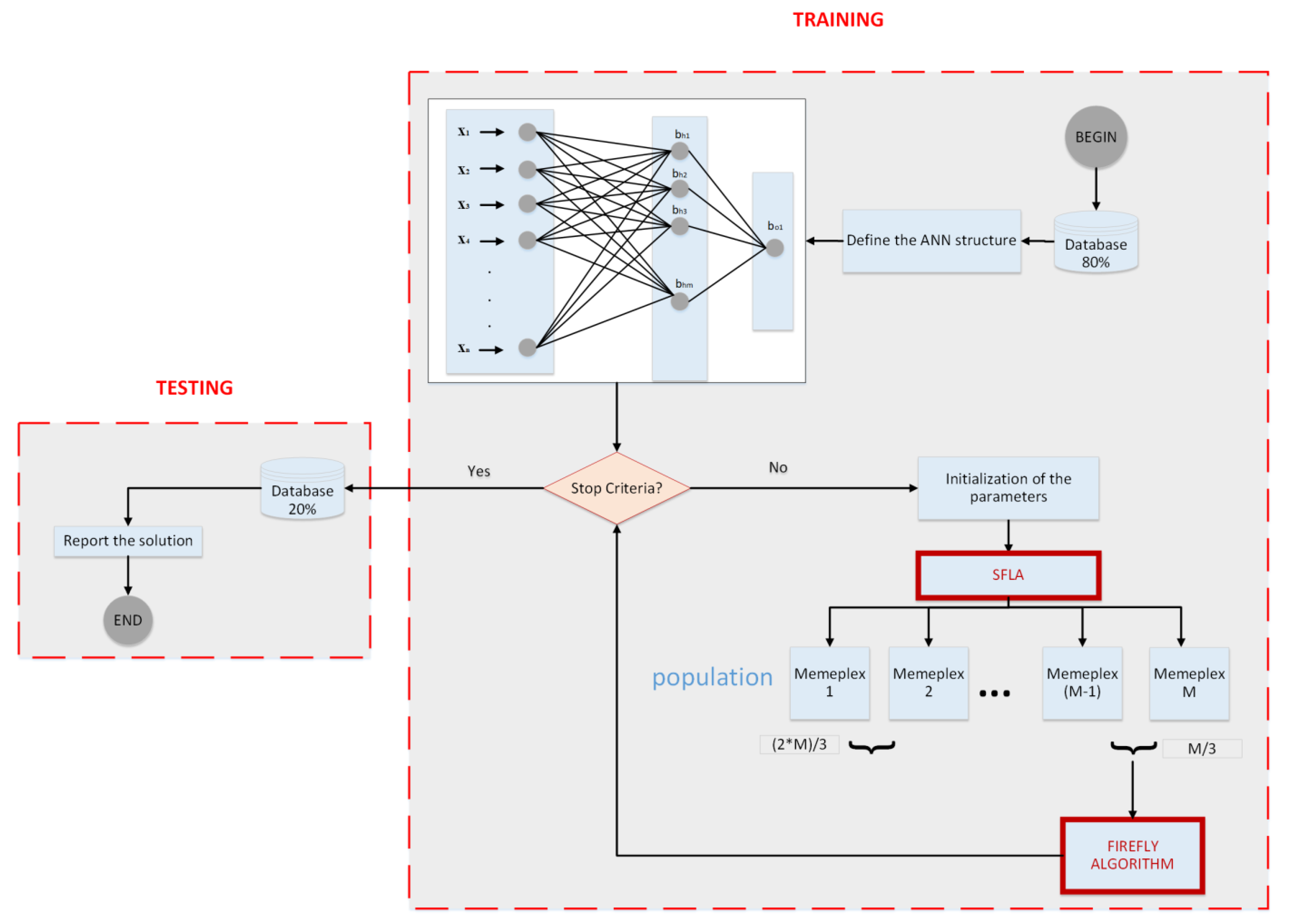
2.2. Design of Proposed Estimation Method

The main purpose of this study is to forecast the CO₂ emission in Türkiye with the minimum error. For this purpose, a new estimation method is proposed in this study and it is developed by optimizing artificial neural networks using metaheuristic optimization algorithms. In order to get the best result from an artificial neural network, the network coefficients should be optimally adjusted. In the proposed estimation method, the coefficients (weights and biases) of the artificial neural network are adjusted with an improved Levy Flight Shuffled Frog-Leaping Algorithm based on the Firefly Algorithm (ILSFLAFA), which is a method developed by using metaheuristics optimization algorithms in a hybrid structure.

In the estimation step, a multilayer feedforward neural network is used. The training of the network coefficients is provided by the proposed hybrid optimization method. Metaheuristic methods in a hybrid structure are used to:

• Improve forecasting performance;
• Increase the ability to train;
• Improve the speed of convergence;
• Find the optimum result in the search space.

Heuristic methods are utilized in the decision-making phase to optimize the bias and weight values of the feedforward multilayer neural network. Each individual in the heuristic methods consists of the weight and bias values of the network structure. Initially, each individual in the search space is created. The fitness value of each individual in the search space is the error value of the network structure obtained by using the values held by that individual in the network. In this step, Normalized Mean Squared Error (NMSE) is used as the error criterion. MSE is calculated as:

$$\mathrm{MSE}=\frac{{{\displaystyle \sum }}_{\mathrm{i}=1}^{\mathrm{n}}{\left({\mathrm{x}}_{\mathrm{actual}}-{\mathrm{x}}_{\mathrm{predicted}}\right)}^2}{\mathrm{n}}$$

(19)

here, ${\mathrm{x}}_{\mathrm{actual}}$ and ${\mathrm{x}}_{\mathrm{predicted}}$ are represents the measured and predicted output values, respectively. $\mathrm{n}$ is the number of samples. The NMSE is obtained by dividing the MSE by the mean-variance of the target rows. A detailed flowchart of the proposed Hybrid Swarm-Based MLNN (HSBNN) as a new estimation method in this work is presented in Figure 3.

3. Results

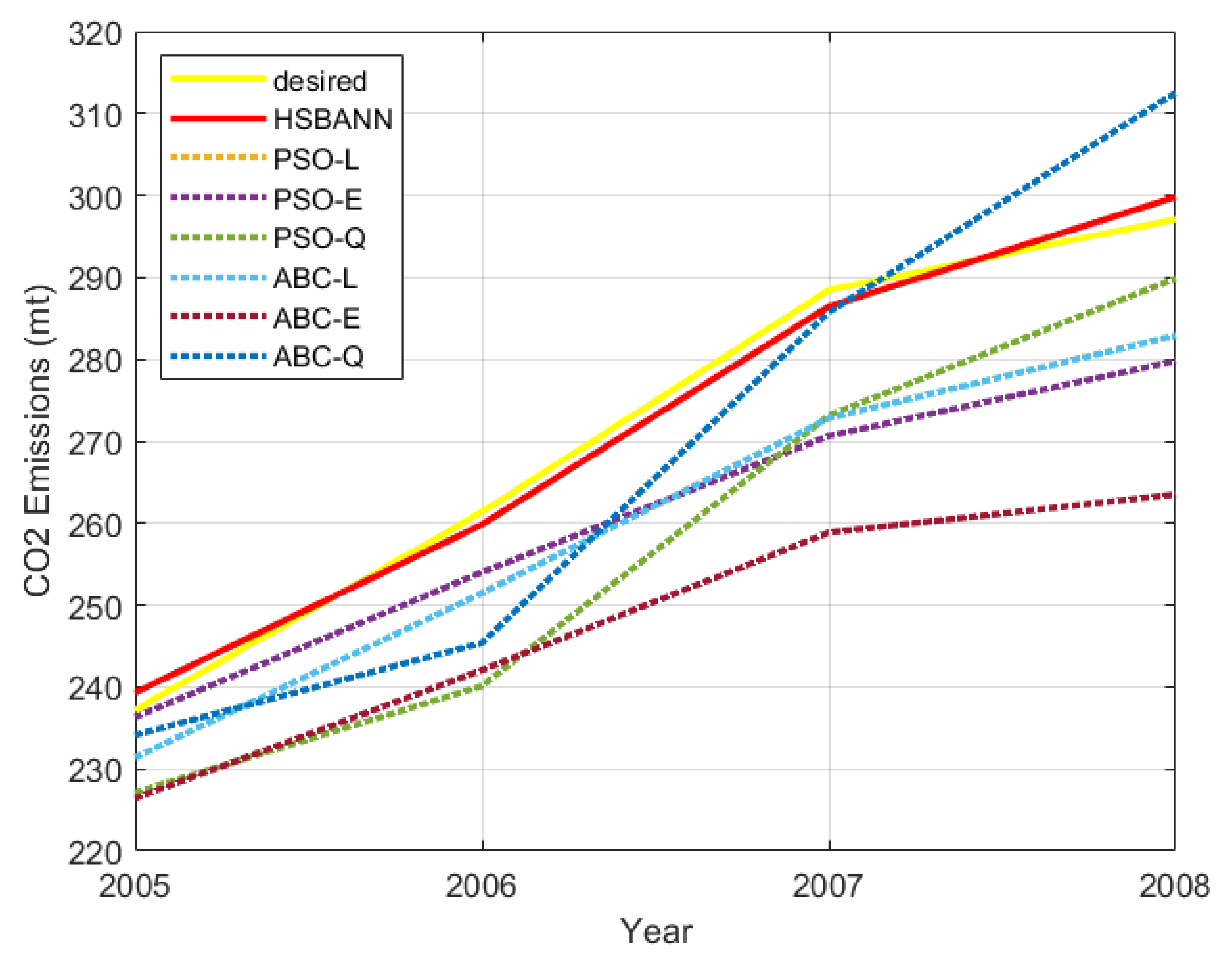
3.1. Comparison of the Proposed Estimation Method

In this work, the training of the Artificial Neural Network (ANN) structure was done with the proposed optimization method. Thanks to the improvement in the optimization method, more successful results are obtained in convergence speed and forecasting performance. The following section has been added to the article to show the improvement in the convergence speed in the proposed optimization method. In this section, the convergence speed and computation time information of the methods are given.

Today, optimization methods in different structures are proposed to solve many real-life engineering problems. Benchmark Functions are used to test the convergence rate, parameter sensitivity and robustness of these methods against uncertainties. Benchmark Functions are test functions with different properties that are used to test the performance of optimization methods from different aspects. These functions are generally accepted in terms of comparison of optimization methods. In this work, benchmark functions are used to show the success and convergence speed of the proposed method as in most optimization studies in the literature. Here, the most frequently used four Benchmark Functions are preferred and the equation, limit values and optimum value information of the functions are given in

Table 2. Benchmark Functions.

Func.	Benchmark Problem	Formulation	Search Range	Initial Range	Global Min.
F1	Sphere	$f\left(x\right)={\displaystyle {\displaystyle \sum }_{i=1}^n}{x}_i^2$	[–100, 100]	[–100, 50]	0
F2	Schwefel 2.22	$f\left(x\right)={\displaystyle {\displaystyle \sum }_{i=1}^n}\left|x_i\right|+{\displaystyle {\displaystyle \prod }_{i=1}^n}\left|x_i\right|$	[–10, 10]	[–10, 5]	0
F3	Sum Square	$f\left(x\right)={\displaystyle {\displaystyle \sum }_{i=1}^n}i{x}_i^2$	[–10, 10]	[–10, 10]	0
F4	Cigar	$f\left(x\right)=x_i^2+{10}^6{\displaystyle {\displaystyle \sum }_{i=2}^n}{x}_i^2$	[–100, 100]	[–100, 100]	0

.

The proposed optimization method (ILSFLAFA) in this work is obtained by hybridizing the Firefly Algorithm (FA) and the Shuffled Frog-Leaping Algorithm (SFLA) and additionally making some improvements. Therefore, in order to demonstrate the success of the proposed method, the results obtained using the Benchmark functions are compared with the results obtained by the FA and SFLA methods. The parameters of the optimization methods are given in

Table 3. Optimization parameters for the optimization algorithms.

Parameters	FA	SFLA	ILSFLAFA
Population size	24	24	24
Fitness evaluations	400	400	400 (100 × 4)
Number of decision variables	30	30	30
Light absorption coefficient	2.0	-	2.0
Attraction coefficient	1.8	-	1.8
Number of Memeplexes	-	6	6
Memeplex Size	-	4	4
Number of Fitness evaluations for local search	-	4	4
Levy index	-	-	2.0

.

In

Table 4. Comparison of the FA, SFLA and ILSFLAFA on unimodal and multimodal Benchmark functions.

		FA	SFLA	ILSFLAFA
F1	best	5.37 × 10−18	8.38 × 10−9	0
	worst	3.30 × 100	8.06 × 10−4	0
	std	7.37 × 10−1	2.93 × 10−4	0
Computation time		1.5791 × 10−13	13.064510	83.375757
F2	best	2.74 × 10−16	2.44 × 10−5	0
	worst	7.50 × 10−3	7.03 × 10−2	0
	std	2.27 × 10−3	2.14 × 10−2	0
Computation time		3.024902	13.188631	87.217499
F3	best	5.42 × 10−201	3.11 × 10−282	0
	worst	1.64 × 10−198	1.69 × 10−274	0
	std	0	0	0
Computation time		2.898312	13.158265	80.099749
F6	best	2.85 × 10−203	3.90 × 10−280	0
	worst	6.87 × 10−199	5.41 × 10−267	0
	std	0	0	0
Computation time		2.877054	13.436169	81.848208

, the results obtained with 400 fitness evaluations for 30-dimensional Benchmark Functions are given. The best optimum values, mean values and standard deviations of the results obtained over 20 runs obtained with the FA, SFLA and the proposed hybrid optimization method are given in Table 4. In each function, the best results are indicated by boldface.

As the results obtained from the benchmark functions are examined, it is seen that the proposed method is generally successful compared to the other two methods. In optimization methods, the convergence speed of that method to find the optimal solution is also important. The convergence speed is of great importance in performance comparison. Convergence graphs are shown in Figure 4, Figure 5, Figure 6 and Figure 7 to compare the convergence rates of the FA, SFLA and proposed method. The results are also given by zooming in order to see the convergence more clearly.

As the numerical results obtained as a result of the application of the FA, SFLA and ILSFLAFA methods to four different Benchmark Functions are examined, the success of the proposed method is clearly seen. In addition, when the graphs in Figure 4, Figure 5, Figure 6 and Figure 7 are examined to compare the converge speeds of the optimization methods, it is seen that the proposed method reaches the optimum solution in the first 100 fitness evaluations.

This work aims to contribute to the studies on this subject by developing an estimation method for Türkiye’s CO₂ emissions in the future. There are different studies carried out to date for the estimation of CO₂ emissions in Türkiye. One of these studies is carried out by Özceylan in 2016 [54]. The CO₂ estimation method is modelled by Özceylan using the linear, exponential and quadratic equation forms. Particle Swarm Optimization (PSO) and Artificial Bee Colony (ABC) approaches are employed in the development of these models. Energy consumption, population, gross domestic product (GDP) and the number of motor vehicles data of Türkiye’s for the years 1980–2008 are used in this estimation model as socioeconomic indicators.

In this work, an artificial neural network-based prediction method has been developed for the estimation of CO₂ emissions. In this developed method, a multilayer feedforward artificial neural network is used. The proposed prediction method is first applied to the data of Özceylan’s article and the results are compared. The data set in Özceylan’s paper is as given in article [54]. The first 25 years of data (1980–2004) are used to validate the models and set the weighting parameters, while the last five years of data (2005–2008) are used to test the models. At the end of the study, relative error is used as the error criterion. The equation for the relative error criterion is as follows:

$$\mathrm{Relative}\mathrm{Error}=\frac{\mathrm{absolute}\mathrm{error}}{\mathrm{actual}\mathrm{value}}=\frac{\left({\mathrm{x}}_{\mathrm{predicted}}-{\mathrm{x}}_{\mathrm{actual}}\right)}{{\mathrm{x}}_{\mathrm{actual}}}$$

(20)

here, ${\mathrm{x}}_{\mathrm{actual}}$ and ${\mathrm{x}}_{\mathrm{predicted}}$ represent the measured and predicted output values, respectively. Özceylan used 40 individuals in the search spaces of swarm-based methods, and the methods ran 10,000 fitness evaluations during the creation of the models.

The feedforward artificial neural network utilized in the study for this data set has four neurons in the input layer, four neurons in the hidden layer and one neuron in the output layer, according to the method provided in the study. The results given at the end of Özceylan’s article, the results obtained with the proposed Hybrid Swarm-Based MLNN (HSBNN) method and the relative errors are as shown in

Table 5. The results obtained with the HSBNN method and the relative errors [54].

	2005	2006	2007	2008
Actual data [55]	237.174	261.357	288.445	297.120
HSBNN	239.3081	259.8382	286.4580	299.8035
Relative Error %	0.8998	−0.5811	−0.6889	0.9032
PSOCO2 linear (PSO-L)	231.399	251.480	272.824	282.906
Relative Error %	−2.435	−3.779	−5.416	−4.784
PSOCO2 exponential (PSO-E)	236.319	254.021	270.648	279.787
Relative Error %	−0.361	−2.807	−6.170	−5.834
PSOCO2 quadratic (PSO-Q)	227.135	240.122	273.136	289.881
Relative Error %	−4.233	−8.125	−5.307	−2.436
ABCCO2 linear (ABC-L)	231.399	251.468	272.806	282.888
Relative Error %	−2.435	−3.784	−5.422	−4.790
ABCCO2 exponential (ABC- E)	226.430	242.060	258.865	263.508
Relative Error %	−4.530	−7.383	−10.255	−11.313
ABCCO2 quadratic (ABC-Q)	234.139	245.389	285.749	312.542
Relative Error %	−1.280	−6.110	−0.935	5.191

.

In the HSBNN method, 40 individuals are used in the study and the training of the network is performed in 1000 fitness evaluations. The optimization parameters of the HSBNN method are given in

Table 6. Optimization parameters of the proposed prediction model.

Parameters	Value	Parameters	Value
Number of input neurons	4	Memeplex Size	4
Number of hidden neurons	6	Number of Fitness evaluations for local search	5
Number of output neurons	1	Levy index	2.0
Population size	24	Light absorption coefficient	1.0
Number of Memeplexes	6	Attraction coefficient	2.0

.

In the test phase, data from 2005 to 2008 are used. The average relative errors of the proposed models are as shown in

Table 7. Average relative errors of proposed models [54].

Prediction Models	Average Relative Errors
HSBNN	0.7682
PSOCO2 linear	4.104
PSOCO2 exponential	3.793
PSOCO2 quadratic	5.025
ABCCO2 linear	4.108
ABCCO2 exponential	8.37
ABCCO2 quadratic	3.379

.

By examining Table 5, it can be seen that the estimation results achieved using various methods are closer to the real values in some cases. The mean relative errors of the results are given in Table 7 so that the method successes may be seen more clearly. The comparison of the results obtained with the HSBNN and methods used in the article is graphically shown in Figure 8.

In the reviewed article, CO₂ estimation is made with six different methods. The HSBNN method proposed in this work is also applied to the same data set. The desired CO₂ emission values and the results obtained from these methods are given in Table 5 and Table 7 and Figure 8. In the estimation results for the years 2005–2008, the ABC^CO2 quadratic model obtained the best result from the methods used in the article. While the average relative error of the prediction result obtained with this model is 3.379, the average relative error value obtained with the HSBNN is 0.7682. When these results are examined in detail, it is clear that the proposed HSBNN method produces more successful and effective results.

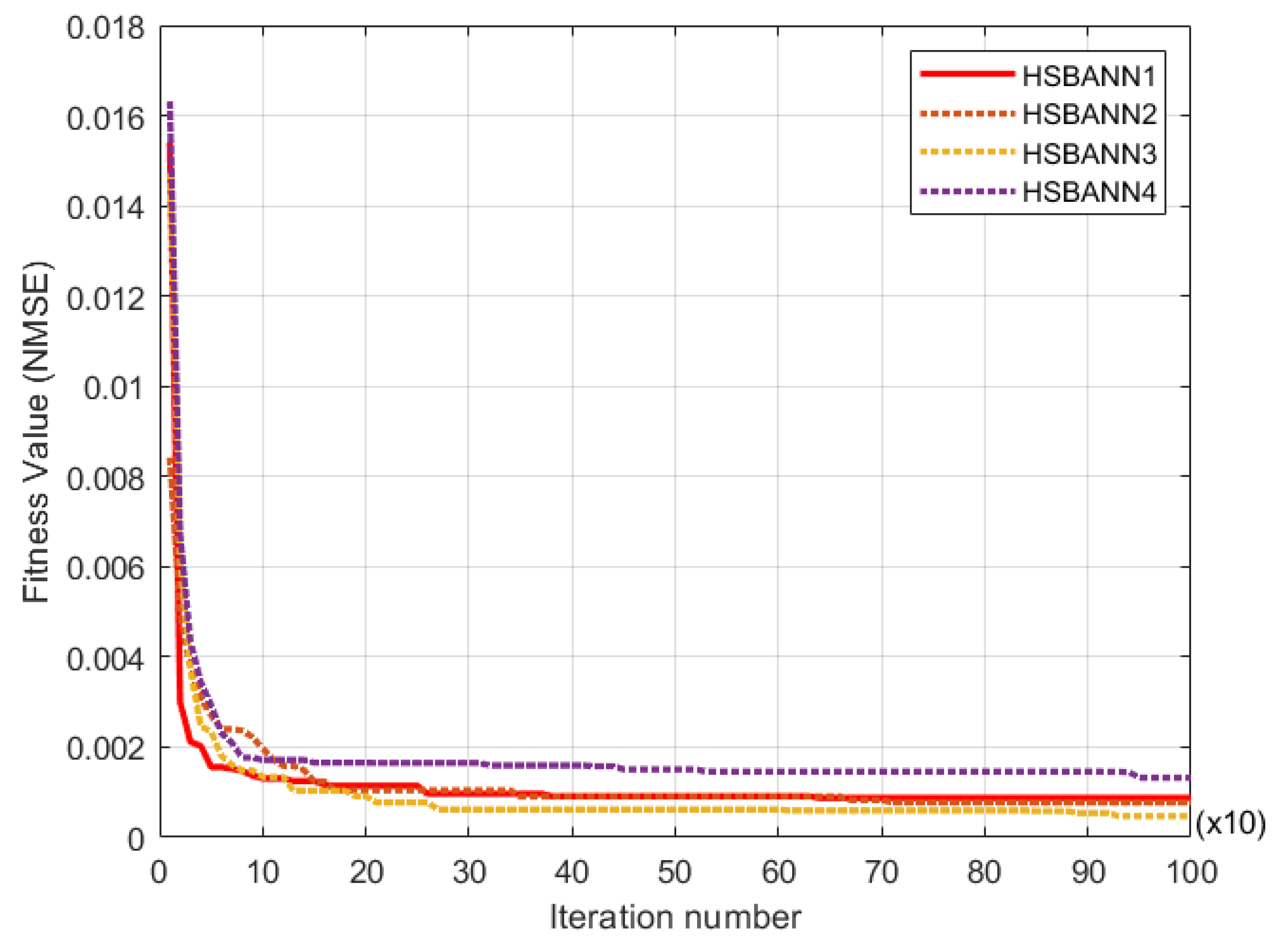
3.2. Prediction of CO₂ Emissions

3.2.1. Dataset

According to the literature, it is seen that socioeconomic factors are used for the estimation of CO₂ emissions. In addition, in this study, the renewable energy factor is also used to estimate the amount of emissions. The data set used in the study was created as follows:

• Year;
• R&D investments [56];
• Renewable energy ratio of total final energy consumption [57];
• Population [58];
• Urbanization [59];
• Number of motor vehicles [60];
• Energy consumption [61];
• GDP [62];
• Amount of CO₂ emissions [63].

The data set is obtained from different institutions. The historical values for the data titles that are desired to be used are limited. The provided data covers the years 1990 to 2018.

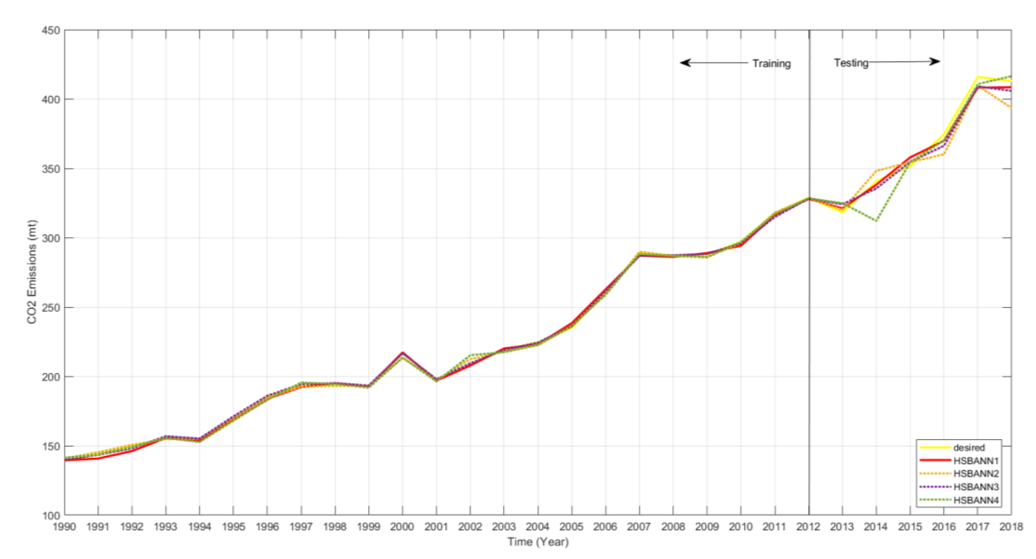
3.2.2. Prediction of the Türkiye’s CO₂ Emissions

In this work, the hybrid swarm-based metaheuristic optimization method is used in four different structures and is used in the training phase of the multilayer feedforward neural network. The number of neurons in the input layer is determined by the data set used in studies using artificial neural network-based approaches. The number of neurons in the output layer is determined by the problem structure. In this study, the number of neurons in the input layer and output layer is determined as 8 and 1, respectively. The input parameters of the network are year, R&D investments, renewable energy ratio of total final energy consumption, population, urbanization, number of motor vehicles, energy consumption and GDP. The output layer of the network is the CO₂ emission amount. At the beginning of the study, the data is divided into two separate subsets. The first set, which involves data from 1990 to 2012, is used for training the proposed forecasting model, while the second set, which involves data from 2013–2018, is employed to test the accuracy of the forecasting model. To estimate the CO₂ emission amount, the ANN structure in the Hybrid Swarm-Based Neural Network (HSBNN) is used in four different ways. In the first proposed method, one hidden layer is used. In the other three methods, there are two layers in the hidden layer. In these four methods, four different estimation methods have been developed by using different neuron numbers in the hidden layers to obtain the best prediction model by examining the obtained results.

When the literature is examined, it is seen that many different methods based on ANN are frequently used for CO₂ emission estimation. In ANN-based methods, the aim is to create a prediction model based on historical data. The accuracy of the created model is also measured using the available data. In this study, the data set obtained from different institutions and databases was used. These institutions and databases have data for the years 1990–2018 in common. Data from 1990–2012 have been used to create the ANN-based forecasting method, and data from 2013–2018 have been used to investigate the accuracy of the proposed method. In the next step, if desired, the ANN-based forecasting method can also be used for forecasting for future years.

Different error criteria are used to show the accuracy of the prediction results. The formulas for the used Mean Absolute Error (MAE), Root Mean Square Error (RMSE), Mean Absolute Percentage Error (MAPE) and Theil’s inequality coefficient (TIC) error criteria are as follows:

Mean absolute error (MAE)

$$\mathrm{MAE}=\frac{1}{\mathrm{n}}{\displaystyle {\displaystyle \sum }_{\mathrm{i}=1}^{\mathrm{n}}}\left|{\mathrm{x}}_{\mathrm{actual}}-{\mathrm{x}}_{\mathrm{predicted}}\right|$$

(21)

Root mean square error (RMSE)

$$\mathrm{RMSE}=\sqrt{\frac{1}{\mathrm{n}}{\displaystyle {\displaystyle \sum }_{\mathrm{i}=1}^{\mathrm{n}}}{\left({\mathrm{x}}_{\mathrm{actual}}-{\mathrm{x}}_{\mathrm{predicted}}\right)}^2}$$

(22)

Mean absolute percentage error (MAPE)

$$\mathrm{MAPE}=\frac{1}{\mathrm{n}}{\displaystyle {\displaystyle \sum }_{\mathrm{i}=1}^{\mathrm{n}}}\left|\frac{{\mathrm{x}}_{\mathrm{actual}}-{\mathrm{x}}_{\mathrm{predicted}}}{{\mathrm{x}}_{\mathrm{predicted}}}\right|$$

(23)

Theil’s inequality coefficient (TIC)

$$\mathrm{TIC}=\frac{\sqrt{\frac{1}{\mathrm{n}}{{\displaystyle \sum }}_{\mathrm{i}=1}^{\mathrm{n}}{\left({\mathrm{x}}_{\mathrm{actual}}-{\mathrm{x}}_{\mathrm{predicted}}\right)}^2}}{\sqrt{\frac{1}{\mathrm{n}}{{\displaystyle \sum }}_{\mathrm{i}=1}^{\mathrm{n}}{\left({\mathrm{x}}_{\mathrm{actual}}\right)}^2}+\sqrt{\frac{1}{\mathrm{n}}{{\displaystyle \sum }}_{\mathrm{i}=1}^{\mathrm{n}}{\left({\mathrm{x}}_{\mathrm{predicted}}\right)}^2}}$$

(24)

here, ${\mathrm{x}}_{\mathrm{actual}}$ and ${\mathrm{x}}_{\mathrm{predicted}}$ represent the measured and predicted output values, respectively. $\mathrm{n}$ is the number of samples.

In ANN-based methods, the aim is to create a prediction model based on historical data. The accuracy of the created model is also measured using the available data. In this study, the data set obtained from different institutions and databases has been used. These institutions and databases have data for the years 1990–2018 in common. Data from 1990–2012 have been used to create the ANN-based forecasting method, and data from 2013–2018 have been used to investigate the accuracy of the proposed method.

In this method, the method used for training the weights and biases of the ANN structure is an optimization method. At each step in the training phase, the error value of the current network structure is calculated, and then the weight and bias values are updated in the step according to that error value. The criterion used to calculate the success of the network at each step in the training phase is the NMSE error criterion. In this way, the training phase of the network is completed.

The multi-layer artificial neural network in the proposed prediction model is used in four different structures in the CO₂ emission estimation phase. In the first model (HSBNN¹), the ANN is designed with 12 neurons in one layer in the hidden layer. The structure of the ANN of this model is 8-12-1. In the second model (HSBNN²), two layers are used in the hidden layer. The number of neurons in these layers is six and four, respectively. Therefore, the number of neurons in the neural network structure is 8-6-4-1. The HSBNN³ model is built with a neural network with six neurons in both hidden layers. Hence, the number of neurons in the network structure is 8-6-6-1. Finally, the hidden layer of the artificial neural network in the HSBNN⁴ model is created as two layers. There are eight neurons in the first hidden layer and four neurons in the second hidden layer. The structure of the neural network of this model is 8-8-4-1. The estimation results obtained with these four different structure methods are as shown in

Table 8. Training and testing errors for four different prediction models.

	No of Neuronsin 1st Hidden Layer	No of Neuronsin 2nd Hidden Layer	Error for Training Data Set	Error for Testing Data Set
			NMSE	MAPE (%)	RMSE	MAE	TIC
HSBNN1	12	-	0.000873	1.2752	5.1107	4.7789	0.0138
HSBNN2	6	4	0.000774	2.2974	10.8183	8.8022	0.0295
HSBNN3	6	6	0.000469	1.6456	6.3267	6.0970	0.0172
HSBNN4	8	4	0.001321	2.4199	12.4193	8.5026	0.0338

.

In this work, a multi-layer artificial neural network is used in the proposed estimation method. In the proposed estimation method, the NMSE value is used as the fitness function during the parameter training of the neural network and the graph of the curves of the obtained NMSE values is shown in Figure 9. It can be seen that the prediction model that found the best result at the end of the training phase is HSBNN³.

Figure 10 shows the comparison of the actual data and proposed four prediction models results of the training and testing data set. The accuracies of the chosen models are difficult to distinguish, but the numbers reveal that the training part is more accurate than the test part.

Comparisons of the performances of prediction methods for the testing set are presented in Figure 11.

Linear regression of the actual CO₂ emission measurement value that is taken from the institution relative to results from prediction models is shown in Figure 12.

The evaluation of the prediction results according to the criteria of linear regression, R² and mean relative error are given in

Table 9. Comparison table of Linear Regression, R² and Relative Error of prediction results.

	Regression	R2	Relative Error (%)
HSBNN1	0.99518	0.9904	1.2752
HSBNN2	0.97661	0.9538	2.2974
HSBNN3	0.99356	0.9872	1.6456
HSBNN4	0.95556	0.9131	2.4199

.

3.2.3. Future Prediction of the Türkiye’s CO₂ emissions

At this stage in the work, the proposed prediction method is used for three different scenarios to the future forecast of CO₂ emissions in Türkiye. The data to be used in this step of the study is set as follows:

R&D investments

The average increase in the last 2 years (according to TurkStat data [56] is preferred for Scenario 1.

The average increase in the last 3 years (according to TurkStat data [56] is preferred for Scenario 2.

The average increase in the last 5 years (according to TurkStat data [56] is preferred for Scenario 3.

Renewable energy ratio

Average rate of increase in the last 3 years (according to Worldbank data [57] is preferred for Scenario 1.

Average rate of increase in the last 5 years (according to Worldbank data ([57] is preferred for Scenario 2.

Average rate of increase in the last 8 years (according to Worldbank data [57] is preferred for Scenario 3.

Population

Estimated population data from TURKSTAT is used [58].

Urbanization

Average values are determined according to the rate of increase in recent years (according to Indexmundi data [59]).

Additionally, the rate of increase in the number of motor vehicles and energy consumption data is taken from Özceylan’s article [54]. In addition, the increased rate of GDP data is taken from Uzlu’s article [64]. The details of the scenarios are presented in

Table 10. Scenarios for Türkiye’s CO₂ emission prediction (approximate growth rates).

	Scenario 1	Scenario 2	Scenario 3
R&D investments [56]	19.42%	22.64%	21.72%
Renewable energy ratio [57]	12.16%	12.27%	12.60%
Population [58]	TurkStat population forecasts	TurkStat population forecasts	TurkStat population forecasts
Urbanization [59]	1.0%	1.05%	1.08%
Number of motor vehicles [54]	3.0%	3.5%	4.0%
Energy consumption [54]	2.0%	2.5%	3.0%
GDP [64]	4.87%	6.37%	7.87%

.

The results of future projections for different scenarios are shown in

Table 11. Future projections of CO₂ emission amount according to scenarios with proposed optimization method.

Year	Scenario 1	Scenario 2	Scenario 3
2018 [63]	412.9700	412.9700	412.9700
2019	419.7500	418.8049	419.2450
2020	427.1719	427.1067	426.2700
2021	434.7241	436.2368	433.4406
2022	442.1495	445.6232	440.4107
2023	449.3373	454.8216	447.0232
2024	455.8839	463.3066	452.8473
2025	460.7198	470.1485	457.0039
2026	464.1629	476.0640	467.5716
2027	469.7298	484.0587	473.9727
2028	478.7903	494.4381	483.6537
2029	490.7800	506.6813	496.0707
2030	504.6270	519.2656	510.0260

. Türkiye’s average CO₂ emission amount in 2030, according to the future CO₂ emission estimation generated with the approach given in this study, is 510 Mt. According to the Paris Agreement, it is aimed to reduce greenhouse gas emissions by 50% by 2030. In this direction, countries need to accurately estimate the amount of CO₂ emissions, which has the most effective ratio in the amount of greenhouse gas emissions and take precautions accordingly.

With the proposed estimation method in the study, emission estimation can be made according to different scenarios. Thus, a step forward for the sustainable world can be taken by taking various precautions.

4. Discussion

Artificial Neural Networks (ANNs) have been used together with optimization methods in recent years due to their high accuracy prediction and classification capability, and their usage in many different fields is increasing rapidly. However, ANN modeling has its own difficulties. Many potential ways can be applied to create and train networks. In this study, SFLA and FA methods have been used in hybrid structures to train ANN variables. In the first step of the study, the ANN model optimized by improved Levy flight SFLA-FA (ILSFLAFA), which was proposed as a new optimization method, was used. The ANN structure was created in four different ways and the analyses were made through these four different proposed estimation methods.

Table 8 and Figure 10 show the results of four different methods proposed in the study. At the end of the training phase, the prediction model that provided the best result was HSBNN³. According to the NMSE criteria, the HSBNN⁴ method has the highest error at the end of the training phase with a value of 0.0013. According to Table 8, the RMSE values of the four approaches proposed for the testing phase are 5.1107, 10.8183, 6.3267 and 12.4193. The MAPE values are also 1.2752%, 2.2974%, 1.6456% and 2.4199%, respectively. Estimated values annually are shown in Figure 11. The results of the HSBNN¹ model are consistent with the trend of actual carbon dioxide emissions from 2013 to 2018, as shown in Table 8 and Figure 10, allowing for a lower error value estimation. As seen in Table 9, estimation results based on linear regression, R² and mean relative error criteria are given here. It is seen that HSBNN¹ has a very small degree of deviation from the true value compared to other methods. The results in Figure 12 and Table 9 show that the results obtained using the HSBNN¹ approach have the best correlation with the values of measured CO₂ emissions.

While creating the scenarios, real data obtained from both the literature and the relevant official institutions/organizations (TURKSTAT—Turkish Statistical Institute) were used. Since no specific situation data about the data was available, unexpected situation analysis was not performed, and the results were obtained realistically according to the normal data situation. According to the future CO₂ emission estimates created using the methodology described in this paper, Türkiye’s average CO₂ emission is predicted. When the future forecast results are examined, it is seen that the highest carbon emission amount is reached in the second scenario. It is seen that the expected increase in renewable energy sources cannot reduce the amount of emissions at the desired rate unless adjustments are made in other parameters. In order to reach the 2030 targets in the Paris Agreement, it is foreseen that measures should be taken by considering the parameters used in this study.

5. Conclusions

The earth is dealing with worldwide crisis as global warming and climate change. The EU and other countries introduce new regulations and sanctions to protect the ecosystem and ensure the sustainability of life in the world. With the European Green Deal, the European Union aims to reduce carbon emissions by 50 percent by 2030 and to zero carbon emissions by 2050. For this purpose, it plans to apply the Carbon Border Adjustment Mechanism to the countries it trades with. Türkiye, one of the countries that trade with the EU, brought the issue of CO₂ emissions to the agenda in order to ensure the continuity of trade and sustainable development before the sanctions begin. The main purpose of this study is to propose a new method that can estimate Türkiye’s emission amount with less error.

The paper offers an ANN-based hybrid approach for predicting the total volume of CO₂ emissions. During the creation of the model, the ANN structure has examined with different layer numbers and neuron numbers. The most suitable ANN structure has been decided to be 8–12–1 from an accuracy point of view. At the end of the study by using the improved estimation method, CO₂ emission estimations has made until 2030 for three different scenarios. The results strongly support the idea that CO₂ emission in Türkiye can be successfully estimated with relevant components including renewable energy consumption. When we look at the limits of the study, in order to make an emission estimation, the data must be collected in a healthy way. Increasing the capacity of public, private and institutional memory is of great importance at this point.

Due to the success of the proposed method, the main advantage of the study is that it will ensure the correct formation of the next strategic plans. At the point of policy implications, the proposed ANN approach can be successfully used to estimate CO₂ emissions in Türkiye. Several policy outcomes can be identified using the proposed method. First, the CO₂ emission estimation will be useful for the research and vision plans of policy-makers in the environmental field and all other actors involved in this field (i.e., national offices, international organizations and non-governmental organizations). Secondly, the fact that one of the parameters includes the rate of use of renewable energy will show the importance of the use in this area on the amount of emissions when creating different forecast scenarios.

References

1. Jenkinson, D.S.; Adams, D.E.; Wild, A. Model estimates of CO2 emissions from soil in response to global warming. Nature 1991, 351, 304–306. [Google Scholar] [CrossRef]
2. Acaravci, A.; Ozturk, I. On the relationship between energy consumption, CO2 emissions and economic growth in Europe. Energy 2010, 35, 5412–5420. [Google Scholar] [CrossRef]
3. Sadorsky, P. The effect of urbanization on CO2 emissions in emerging economies. Energy Econ. 2014, 41, 147–153. [Google Scholar] [CrossRef]
4. Azomahou, T.; Laisney, F.; Van, P.N. Economic development and CO2 emissions: A nonparametric panel approach. J. Public Econ. 2006, 90, 1347–1363. [Google Scholar] [CrossRef] [Green Version]
5. Gregg, J.S.; Andres, R.J.; Marland, G. China: Emissions pattern of the world leader in CO2 emissions from fossil fuel consumption and cement production. Geophys. Res. Lett. 2008, 35, 2887. [Google Scholar] [CrossRef]
6. Ozturk, I.; Acaravci, A. CO2 emissions, energy consumption and economic growth in Turkey. Renew. Sustain. Energy Rev. 2010, 14, 3220–3225. [Google Scholar] [CrossRef]
7. Arouri, M.E.H.; Youssef, A.B.; M’Henni, H.; Rault, C. Energy consumption, economic growth and CO2 emissions in Middle East and North African countries. Energy Policy 2012, 45, 342–349. [Google Scholar] [CrossRef] [Green Version]
8. European Commission. Living Well, within the Limits of Our Planet. 7th EAP—The New General Union Environment Action Programme to 2020. 2014. Available online: https://ec.europa.eu/environment/pubs/pdf/factsheets/7eap/en.pdf (accessed on 2 March 2022).
9. Ministry of Trade of the Republic of Türkiye. Available online: https://ticaret.gov.tr/data/60f1200013b876eb28421b23/MUTABAKAT%20YE%C5%9E%C4%B0L.pdf (accessed on 2 March 2022).
10. Skjærseth, J.B. Towards a European Green Deal: The evolution of EU climate and energy policy mixes. Int. Environ. Agreem. Politi-Law Econ. 2021, 21, 25–41. [Google Scholar] [CrossRef]
11. Hafner, M.; Raimondi, P.P. Priorities and challenges of the EU energy transition: From the European Green Package to the new Green Deal. Russ. J. Econ. 2020, 6, 374–389. [Google Scholar] [CrossRef]
12. Shan, Y.; Ou, J.; Wang, D.; Zeng, Z.; Zhang, S.; Guan, D.; Hubacek, K. Impacts of COVID-19 and fiscal stimuli on global emissions and the Paris Agreement. Nat. Clim. Chang. 2020, 11, 200–206. [Google Scholar] [CrossRef]
13. Zabojnik, S.; Hricovsky, M. Balancing the Slovak Energy Market After the Adoption of “Fit for 55 Package”. In SHS Web of Conferences. EDP Sci. 2021, 129, 05015. Available online: https://www.shs-conferences.org/articles/shsconf/pdf/2021/40/shsconf_glob2021_05015.pdf (accessed on 2 March 2022).
14. Vinck, N. The Fit for 55 Package and the European Climate Ambitions An Assessment of Their Impacts on the European Metallurgical Silicon Industry. In Proceedings of the Silicon for the Chemical & Solar Industry XVI 2022, Trondheim, Norway, 14–16 June 2022. [Google Scholar]
15. Bäckstrand, K. Towards a Climate-Neutral Union by 2050? The European Green Deal, Climate Law, and Green Recovery. In Routes to a Resilient European Union; Palgrave Macmillan: Cham, Switzerland, 2022; pp. 39–61. [Google Scholar] [CrossRef]
16. Available online: https://data.tuik.gov.tr/Bulten/Index?p=Greenhouse-Gas-Emissions-Statistics-1990-2019-37196 (accessed on 2 March 2022).
17. Ye, L.; Yang, D.; Dang, Y.; Wang, J. An enhanced multivariable dynamic time-delay discrete grey forecasting model for predicting China's carbon emissions. Energy 2022, 249, 123681. [Google Scholar] [CrossRef]
18. Radojević, D.; Pocajt, V.; Popović, I.; Perić-Grujić, A.; Ristić, M. Forecasting of Greenhouse Gas Emissions in Serbia Using Artificial Neural Networks. Energy Sources Part A Recover. Util. Environ. Eff. 2013, 35, 733–740. [Google Scholar] [CrossRef]
19. Bakay, M.S.; Ağbulut, Ü. Electricity production based forecasting of greenhouse gas emissions in Turkey with deep learning, support vector machine and artificial neural network algorithms. J. Clean. Prod. 2020, 285, 125324. [Google Scholar] [CrossRef]
20. Antanasijević, D.Z.; Ristić, M.; Perić-Grujić, A.A.; Pocajt, V.V. Forecasting GHG emissions using an optimized artificial neural network model based on correlation and principal component analysis. Int. J. Greenh. Gas Control 2014, 20, 244–253. [Google Scholar] [CrossRef]
21. Ren, F.; Long, D. Carbon emission forecasting and scenario analysis in Guangdong Province based on optimized Fast Learning Network. J. Clean. Prod. 2021, 317, 128408. [Google Scholar] [CrossRef]
22. Qiao, W.; Lu, H.; Zhou, G.; Azimi, M.; Yang, Q.; Tian, W. A hybrid algorithm for carbon dioxide emissions forecasting based on improved lion swarm optimizer. J. Clean. Prod. 2019, 244, 118612. [Google Scholar] [CrossRef]
23. Alam, T.; AlArjani, A. Forecasting CO2 Emissions in Saudi Arabia Using Artificial Neural Network, Holt-Winters Exponential Smoothing, and Autoregressive Integrated Moving Average Models. In Proceedings of the 2021 International Conference on Technology and Policy in Energy and Electric Power (ICT-PEP), Yogyakarta, Indonesia, 29–30 September 2021; pp. 125–129. [Google Scholar] [CrossRef]
24. Jena, P.R.; Managi, S.; Majhi, B. Forecasting the CO2 Emissions at the Global Level: A Multilayer Artificial Neural Network Modelling. Energies 2021, 14, 6336. [Google Scholar] [CrossRef]
25. Azadeh, A.; Sheikhalishahi, M.; Hasumi, M. A hybrid intelligent algorithm for optimum forecasting of CO2 emission in complex environments: The cases of Brazil, Canada, France, Japan, India, UK and US. World J. Eng. 2015, 12, 237–246. [Google Scholar] [CrossRef]
26. Heydari, A.; Garcia, D.A.; Keynia, F.; Bisegna, F.; De Santoli, L. Renewable Energies Generation and Carbon Dioxide Emission Forecasting in Microgrids and National Grids using GRNN-GWO Methodology. Energy Procedia 2019, 159, 154–159. [Google Scholar] [CrossRef]
27. Zhou, J.; Xu, X.; Li, W.; Guang, F.; Yu, X.; Jin, B. Forecasting CO2 Emissions in China’s Construction Industry Based on the Weighted Adaboost-ENN Model and Scenario Analysis. J. Energy 2019, 2019, 8275491. [Google Scholar] [CrossRef] [Green Version]
28. Guo, J.; Liu, W.; Tu, L.; Chen, Y. Forecasting carbon dioxide emissions in BRICS countries by exponential cumulative grey model. Energy Rep. 2021, 7, 7238–7250. [Google Scholar] [CrossRef]
29. Javed, S.A.; Cudjoe, D. A novel grey forecasting of greenhouse gas emissions from four industries of China and India. Sustain. Prod. Consum. 2021, 29, 777–790. [Google Scholar] [CrossRef]
30. Ahmadi, M.H.; Jashnani, H.; Chau, K.-W.; Kumar, R.; Rosen, M.A. Carbon dioxide emissions prediction of five Middle Eastern countries using artificial neural networks. Energy Sources Part A Recover. Util. Environ. Eff. 2019, 16, 1–13. [Google Scholar] [CrossRef]
31. Ma, X.; Jiang, P.; Jiang, Q. Research and application of association rule algorithm and an optimized grey model in carbon emissions forecasting. Technol. Forecast. Soc. Chang. 2020, 158, 120159. [Google Scholar] [CrossRef]
32. Li, K.; Xiong, P.; Wu, Y.; Dong, Y. Forecasting greenhouse gas emissions with the new information priority generalized accumulative grey model. Sci. Total Environ. 2021, 807, 150859. [Google Scholar] [CrossRef] [PubMed]
33. Şahin, U. Forecasting of Turkey’s greenhouse gas emissions using linear and nonlinear rolling metabolic grey model based on optimization. J. Clean. Prod. 2019, 239, 118079. [Google Scholar] [CrossRef]
34. Liu, Z.; Jiang, P.; Wang, J.; Zhang, L. Ensemble system for short term carbon dioxide emissions forecasting based on multi-objective tangent search algorithm. J. Environ. Manag. 2021, 302, 113951. [Google Scholar] [CrossRef] [PubMed]
35. Khoshnevisan, B.; Rafiee, S.; Omid, M.; Yousefi, M.; Movahedi, M. Modeling of energy consumption and GHG (greenhouse gas) emissions in wheat production in Esfahan province of Iran using artificial neural networks. Energy 2013, 52, 333–338. [Google Scholar] [CrossRef]
36. Antanasijević, D.; Pocajt, V.; Ristić, M.; Perić-Grujić, A. Modeling of energy consumption and related GHG (green-house gas) intensity and emissions in Europe using general regression neural networks. Energy 2015, 84, 816–824. [Google Scholar] [CrossRef]
37. Acheampong, A.O.; Boateng, E.B. Modelling carbon emission intensity: Application of artificial neural network. J. Clean. Prod. 2019, 225, 833–856. [Google Scholar] [CrossRef]
38. Yang, H.; O’Connell, J.F. Short-term carbon emissions forecast for aviation industry in Shanghai. J. Clean. Prod. 2020, 275, 122734. [Google Scholar] [CrossRef]
39. Ho, H.-X.T. Forecasting of CO2 Emissions, Renewable Energy Consumption and Economic Growth in Vietnam Using Grey Models. In Proceedings of the 2018 4th International Conference on Green Technology and Sustainable Development (GTSD), Ho Chi Minh City, Vietnam, 23–24 November 2018; pp. 452–455. [Google Scholar] [CrossRef]
40. Eusuff, M.M.; Lansey, K. Optimization of Water Distribution Network Design Using the Shuffled Frog Leaping Algorithm. J. Water Resour. Plan. Manag. 2003, 129, 210–225. [Google Scholar] [CrossRef]
41. Eusuff, M.; Lansey, K.; Pasha, F. Shuffled frog-leaping algorithm: A memetic meta-heuristic for discrete optimization. Eng. Optim. 2006, 38, 129–154. [Google Scholar] [CrossRef]
42. Yang, X.S. Firefly algorithm. In Nature-Inspired Metaheuristic Algorithms, 2nd ed.; Luniver Press: Frome, UK, 2008; pp. 79–90. [Google Scholar]
43. Senthilnath, J.; Omkar, S.; Mani, V. Clustering using firefly algorithm: Performance study. Swarm Evol. Comput. 2011, 1, 164–171. [Google Scholar] [CrossRef]
44. Yang, X.-S.; Deb, S. Cuckoo Search via Lvy flights. In Proceedings of the 2009 World Congress Nature & Biologically Inspired Computing (NaBIC), Coimbatore, India, 9–11 December 2009; pp. 210–214. [Google Scholar] [CrossRef]
45. Senthilnath, J.; Das, V.; Omkar, S.N.; Mani, V. Clustering using levy flight cuckoo search. In Proceedings of the Seventh International Conference on Bio-Inspired Computing: Theories and Applications (BIC-TA 2012), Dehli, India, 3 July 2013; pp. 65–75. [Google Scholar]
46. Baskan, O. Determining Optimal Link Capacity Expansions in Road Networks Using Cuckoo Search Algorithm with Lévy Flights. J. Appl. Math. 2013, 2013, 1–11. [Google Scholar] [CrossRef]
47. Lan, K.; Liu, L.; Li, T.; Chen, Y.; Fong, S.; Marques, J.A.L.; Tang, R. Multi-view convolutional neural network with lead-er and long-tail particle swarm optimizer for enhancing heart disease and breast cancer detection. Neural Comput. Appl. 2020, 32, 15469–15488. [Google Scholar] [CrossRef]
48. Hariya, Y.; Kurihara, T.; Shindo, T.; Jin’No, K. Lévy flight PSO. In Proceedings of the 2015 IEEE congress on evolutionary computation (CEC), Sendai, Japan, 25–28 May 2015; pp. 2678–2684. [Google Scholar] [CrossRef]
49. Hassanzadeh, T.; Vojodi, H.; Moghadam, A.M.E. A Multilevel Thresholding Approach Based on Levy-Flight Firefly Algorithm. In Proceedings of the 2011 7th Iranian Conference on Machine Vision and Image Processing, Tehran, Iran, 16–17 November 2011; pp. 1–5. [Google Scholar] [CrossRef]
50. Liu, S.; Wang, Y. A Lévy Flight Based Firefly Algorithm for Multilevel Thresholding Image Segmentation. J. Phys. Conf. Ser. 2021, 1865, 2098. [Google Scholar] [CrossRef]
51. Rajpoot, V.; Chitrakoot, M.G.C.G.V.; Tiwari, A.; Mishra, B. AMSFLO: Optimization Based Efficient Approach For Assosia-tion Rule Mining. Int. J. Comput. Sci. Inf. Secur. (IJCSIS) 2018, 16, 147–154. [Google Scholar]
52. Tang, D.; Yang, J.; Dong, S.; Liu, Z. A lévy flight-based shuffled frog-leaping algorithm and its applications for continuous optimization problems. Appl. Soft Comput. 2016, 49, 641–662. [Google Scholar] [CrossRef]
53. Jensi, R.; Jiji, G.W. An enhanced particle swarm optimization with levy flight for global optimization. Appl. Soft Comput. 2016, 43, 248–261. [Google Scholar] [CrossRef]
54. Zceylan, E. Forecasting CO2 emission of Turkey: Swarm intelligence approaches. Int. J. Glob. Warming 2016, 9, 337–361. [Google Scholar] [CrossRef]
55. Indexmundi. Available online: https://www.indexmundi.com/facts/indicators/EN.ATM.CO2E.KT (accessed on 23 October 2014).
56. Turkish Statistical Institute (TURKSTAT). Available online: https://data.tuik.gov.tr/Bulten/Index?p=Arastirma-Gelistirme-Faaliyetleri-Arastirmasi-2020-37439 (accessed on 2 March 2022).
57. World Bank. Available online: https://data.worldbank.org/indicator/EG.FEC.RNEW.ZS?locations=TR (accessed on 2 March 2022).
58. Indexmundi. Available online: https://www.indexmundi.com/Turkey/population.html (accessed on 2 March 2022).
59. Available online: https://www.indexmundi.com/facts/Turkey/urban-population (accessed on 2 March 2022).
60. Turkish Statistical Institute (TURKSTAT). Available online: https://data.tuik.gov.tr/Bulten/Index?p=Motorlu-Kara-Tasitlari-Aralik-2020-37410#:~:text=T%C3%9C%C4%B0K%20Kurumsal&text=T%C3%BCrkiye’de%202020%20y%C4%B1l%C4%B1nda%20bir,bin%20577%20adet%20art%C4%B1%C5%9F%20ger%C3%A7ekle%C5%9Fti (accessed on 2 March 2022).
61. US Energy Information Administration (EIA). Available online: https://www.eia.gov/international/data/country/TUR/total-energy/total-energy-consumption?pd=44&p=0000000010000000000000000000000000000000000000000000000000u06&u=0&f=A&v=mapbubble&a=-&i=none&vo=value&&t=C&g=none&l=249--230&s=315532800000&e=1546300800000 (accessed on 2 March 2022).
62. World Bank. Available online: https://data.worldbank.org/indicator/NY.GDP.MKTP.KD.ZG?locations=TR (accessed on 2 March 2022).
63. World Bank. Available online: https://data.worldbank.org/indicator/EN.ATM.CO2E.KT?locations=TR (accessed on 2 March 2022).
64. Uzlu, E. Estimates of greenhouse gas emission in Turkey with grey wolf optimizer algorithm-optimized artificial neural networks. Neural Comput. Appl. 2021, 33, 13567–13585. [Google Scholar] [CrossRef]
Figure 1. Structure of the division of the population into memeplexes.
Sustainability 14 15595 g001
Figure 2. General flow diagram of the hybrid optimization procedure.
Sustainability 14 15595 g002
Figure 3. Flowchart of the proposed Hybrid Swarm-Based ANN method.
Sustainability 14 15595 g003
Figure 4. Convergence graphs for Sphere function (a) for 1000 iterations (b) zoomed part.
Sustainability 14 15595 g004
Figure 5. Convergence graphs of Schwefel 2.22 function (a) for 1000 iterations (b) zoomed part.
Sustainability 14 15595 g005
Figure 6. Convergence graphs of Sum Square function (a) for 1000 iterations (b) zoomed part.
Sustainability 14 15595 g006
Figure 7. Convergence graphs of Cigar function (a) for 1000 iterations (b) zoomed part.
Sustainability 14 15595 g007
Figure 8. Comparison of the desired data and the proposed models [54].
Sustainability 14 15595 g008
Figure 9. The fitness function curves of the proposed prediction algorithms.
Sustainability 14 15595 g009
Figure 10. Comparison of the actual data and proposed prediction model results (for training and testing data set).
Sustainability 14 15595 g010
Figure 11. Comparison of the actual data and proposed prediction model results (for testing data set).
Sustainability 14 15595 g011
Figure 12. Linear regression graphs of the prediction methods ((a) HSBNN1, (b) HSBNN2, (c) HSBNN3 and (d) HSBNN4).
Sustainability 14 15595 g012