Article

Construction of Commuters’ Multi-Mode Choice Model Based on Public Transport Operation Data

School of Automobile and Traffic Engineering, Wuhan University of Science and Technology, Wuhan 430065, China
*
Author to whom correspondence should be addressed.
Sustainability 2022, 14(22), 15455; https://doi.org/10.3390/su142215455
Submission received: 1 November 2022 / Revised: 12 November 2022 / Accepted: 15 November 2022 / Published: 21 November 2022
(This article belongs to the Section Sustainable Transportation)

Abstract

:
Travel mode selection is a crucial aspect of traffic distribution and forecasting in a comprehensive transportation system, which has significant implications for resource allocation and optimal management. As commuters are the main part of urban travel, studying the factors that affect their choice of transport mode plays a crucial role in urban traffic management and planning. Based on public transport operation data, a travel chain is created by identifying boarding stations, alighting stations, and transfer behaviors, and includes detailed travel information. The regression and correlation coefficients of departures and arrivals at stations are confirmed to be 0.98 and 0.92 in the presented data, indicating the viability of the recognition method. Then, multiple travel modes are identified based on the origin and destination, and the proportion of mode selection is determined by the actual travel chain. Using maximum likelihood estimation (MLS) and NLOGIT software, the random parameter logit (RPL) mode is used to estimate the relationship between travel mode selection and characteristic variables such as travel time, distance, cost, comfort, walking distance, and waiting time. The results indicate that walking distance, travel distance, and comfort have a greater influence on travel choice, and that walking distance is a random parameter with a normal distribution, reflecting the diversity of commuters. In addition, this paper discusses the influence degree of the change of characteristic variables of a transport mode on the choice between it and other modes. These results can be used as reference for relevant departments to make measures to improve the overall efficiency of the urban transportation system.

1. Introduction

Travel mode selection is an essential research topic in urban transportation planning and management, as it partially determines the structure of urban transportation modes. Predicting travel demand and flow distribution is dependent on the mechanism and influencing factors of travel mode selection. Research on travel behavior is crucial for enhancing the structure of urban transportation modes, optimizing the network layout of an integrated transportation system, and enhancing the operating efficiency of a comprehensive transportation system.
Existing research on travel mode selection behavior focuses primarily on the following categories. On the one hand, the probability prediction model is constructed based on the internal rules of travelers’ mode selection behavior, and the sharing rate of each mode of transportation can be estimated using a disaggregated model or game theory [1,2]. On the other hand, some scholars analyze influencing factors on travel choice, focusing on travel characteristics such as travel time, distance, and cost [3,4,5], as well as personal attributes such as age, gender, and income [6,7], so as to make better use of the advantages of different travel modes and enhance the operational efficiency of the integrated transportation system. On this basis, researchers also examine the impact on residents’ travel choices under special circumstances, such as parking fee policies [8,9], congestion fee policies [10,11], the outbreak of COVID-19 [12,13], and climate change [14,15]. However, these works focus on the identification of factors and how they influence travel behavior, ignoring the construction of models and the extraction of influence factors, which directly impacts the precision of model parameter calibration and the rationality of subsequent flow distribution. Therefore, this paper will improve upon the two aspects of model construction and data extraction.
In terms of models, the logit model with stochastic utility maximization, such as multinomial logit (MNL), nested logit (NL), and cross-nested logit (CNL), is most frequently applied to the selection of travel modes [16,17,18]. However, these models assume that everyone’s travel preferences are identical and the parameters of the independent variables are fixed, which is inconsistent with the actual situation. The random parameter logit (RPL) model permits parameters to vary with individuals, taking into account the diversity of residents’ travel preferences, and avoids the limitations of independent and irrelevant alternatives (IIA) [19]. For parameter calibration, maximum likelihood estimation (MLE) is superior to the generalized matrix method (GMM) [20] and Bayesian estimation [21] in terms of convergence and deviation, and it can more accurately reflect the real situation of the model when dealing with a large amount of data [22,23]. Therefore, this paper adopts the RPL model as the travel choice model and estimates its parameters using MLE.
In terms of data source, data used to describe travel choices are usually derived from questionnaires or survey reports [24,25], and residents’ personal and socioeconomic characteristics can be obtained in greater detail. Nevertheless, the survey data suffer from high subjectivity, low precision, and a small sample size [26]. Several scholars have confirmed that travelers’ multi-day travel behaviors are inconsistent [27,28,29], but the survey data is limited to specific scenarios and cannot describe the variety of multi-day travel options. With the advancement of data collection and storage technologies, transport data now contain a greater quantity of travel information; however, its application in travel behavior has primarily focused on travel purpose inference [30,31], travel pattern mining [32,33], traffic OD matrix estimation [34,35], etc. It has been demonstrated that this travel information—in particular, the travel chain—accurately reflects actual travel choices and provides accurate information such as travel mode, time, and location [36]. However, it has been applied less frequently to the analysis and modeling of travel mode selection in previous studies. Therefore, this paper takes this aspect into consideration and extracts more accurate travel characteristics from the travel chain, which will serve as the input of the selection model.
The development and construction of a subway increases the frequency with which residents utilize various modes of public transportation to fulfill their travel needs. Most studies assume that residents have at most one transfer when traveling by public transport [37], but there may be multiple travel stages in practice, resulting in diverse travel patterns that are difficult to categorize. In the meantime, not all travel patterns are suitable for individuals due to the uneven growth of public transport. This paper focuses on the analysis of commuters’ choice between public and private transport modes and does not consider the selection of multiple travel patterns within the public transportation system. The acquisition of private transport data is both expensive and challenging. Observations of vehicles on the road indicate, however, that for the same segment, the passing times of cars and buses with comparable entry times are essentially identical, indicating that their average speeds are similar. Consequently, in the absence of private transport data, one or more buses can be used to represent the driving condition of automobiles, which is another innovation of this paper.
Urban planning and development, as well as road network construction and layout, will alter the travel status of residents, including the distribution of travel flow and the market share of travel mode, etc., necessitating a re-prediction of the travel OD and an analysis of residents’ travel preferences. Traditional survey data cannot overcome the limitations of poor timeliness and small sample size, so this paper utilizes travel information from public transport data to identify boarding stations, alighting stations, and transfer behaviors. On the basis of the public transport travel chain, the round-trip and closed travel characteristics of residents can be used to supplement the travel situation of other modes of transportation. Using the RPL model, a commuter’s multi-mode choice model based on travel chains can be constructed, and its feasibility and dependability are illustrated with an example. By analyzing parameter calibration results, traffic managers are able to take targeted actions to improve the level of public transport operation, as well as plan transportation development and infrastructure construction to enhance residents’ travel satisfaction.
The remainder of the paper is structured as follows: Section 2 introduces the background and methodology, including a data description, method for identifying commuters, and methodology framework. Section 3 describes the extraction process of the public transportation travel chain from the boarding station, alighting station, and transfer behavior. Section 4 clarifies and explains the definition and calculation of the influencing factors. In Section 5, the data are applied to the model of travel mode selection, and the calibration outcomes are analyzed. Section 6 summarizes the conclusions and suggestions for relevant departments.

2. Background and Methodology

2.1. Data Description

Jimo District is located in the northeast of the Chinese city of Qingdao, with a geographical area of 1793 km2 and a population of 1.24 million. Its economic and urban transportation development is at the forefront of all districts in Qingdao. Therefore, the datasets of Jimo’s public transport system on weekdays in May 2018 are taken as the experimental data. In urban public transport systems, three types of public transport operation data can be obtained: IC card data, vehicle GPS data, and station location data. Below are detailed descriptions of these data sets.
  • Bus IC Card data: Passengers make a transaction on the payment device when they board the bus, but not when they exit; therefore, only a portion of the boarding information is recorded on the IC card, such as line ID, card ID, card style, swiping time, transaction amount, driver card ID, and POS ID. In addition, the boarding and alighting stations are determined by combining bus IC card data with bus GPS data and station location data.
  • Bus GPS data: The GPS device installed on the bus records the vehicle’s location and time every ten seconds; this data contains the entire space-time trajectory. The main fields of bus GPS data include the license plate number, bus line ID, time, speed, running direction, and longitude and latitude. However, the arrival time of vehicles at each station cannot be obtained directly.
  • Bus station location data: A station may belong to multiple bus lines, and stations with the same name may be located in different places. This dataset contains the spatial information of each station on each line, allowing for the effective avoidance of identification errors resulting from the aforementioned circumstances. The main fields include the station ID, station name, line ID, and longitude and latitude.
  • Subway IC card data: Passengers must swipe their card at the turnstile when entering or exiting the subway station. Since the transfer occurs within the station, no additional swiping records will be created. Unlike bus IC card data, subway IC card data indicates whether passengers are entering or exiting the station.
As a sample, the public transportation data for a month’s weekdays are extracted. The bus and subway service hours in this area are, respectively, 5:30–22:00 and 6:00–23:15. During storage and transmission, invalid data may be produced as a result of obsolete or broken devices and an unstable network. To improve the precision of sample data, it is necessary to preprocess the original data by removing invalid data records containing “null,” “,” and “0” that are not in the running time. The first duplicate data record is kept and the others are deleted. In addition, in order to reduce the complexity of data processing, the following operations are carried out: deletion of redundant information, standardization of the data storage format, and exclusion of GPS data records with no motion.
After data processing, the total number of card records is 909,004, which equates to an average of 454,450 card records per day, or approximately 455,000 passengers per day. Assuming that each passenger has only one card, the total number of IC cards is 26,591; this indicates that 26,591 residents traveled during the specified time frame.
For the purpose of factor calculation, the study area is divided into a number of traffic zones, after which their centroids are determined. With the aid of OSM (OpenStreetMap) data and ArcGIS software, it is possible to obtain 1268 traffic zones (see Figure 1), and the centroids of some traffic zones are depicted in Figure 2.

2.2. Commuter Identification

Commuting is the main part of urban residents’ travel, and it is of great significance to study commuters’ travel behavior for optimizing urban traffic layout and alleviating road congestion [38]. However, passengers are simply divided into the categories of student, older, and ordinary users in IC card data (See Table 1), and it is not possible to directly judge who are commuters; therefore, commuter identification is needed.
Commuters are typically defined as individuals who travel frequently between their residence and place of employment [39]. Commuters have greater spatiotemporal regularity than other travelers, which is primarily reflected in the following aspects:
  • They travel everyday unless exceptional circumstances arise.
  • Departure times are primarily in the morning and evening rush hours.
  • In general, the first boarding station is near the residence and the last boarding station is near the workplace.
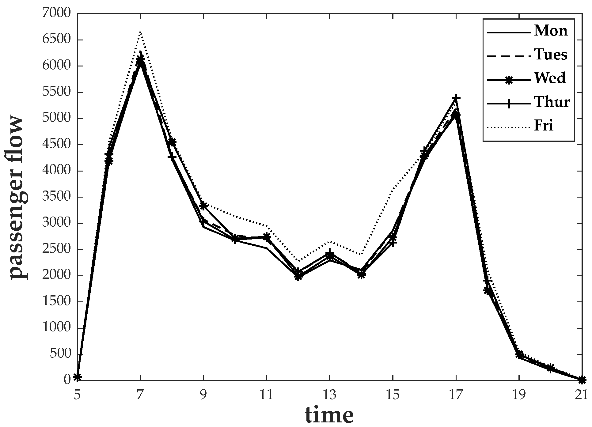
The most intuitive and effective method for identifying commuters is feature identification, which sets rules based on commuting characteristics. Fan et al. [40] considered the number of active travel days and defined commuters as individuals who travel more than 15 days per month. Mei et al. [41] identified commuters using the first departure time, the last departure time, and the number of travel days as the characteristic indices of a random forest classification algorithm. Travel days and departure time are typical commuter characteristics. For passengers with continuous travel, if the travel days D t exceeds 60% of the total number of days D total , namely, D t / D total   60 % , and departure time is mostly in the peak hours, they will be considered commuters. According to Figure 3, the morning and evening peak hours are, respectively, 6:30–9:00 and 16:30–18:00. Figure 4 depicts the algorithm’s detailed procedure, which eliminates 5215 commuters and 361,224 travel records.

2.3. Methodology Framework

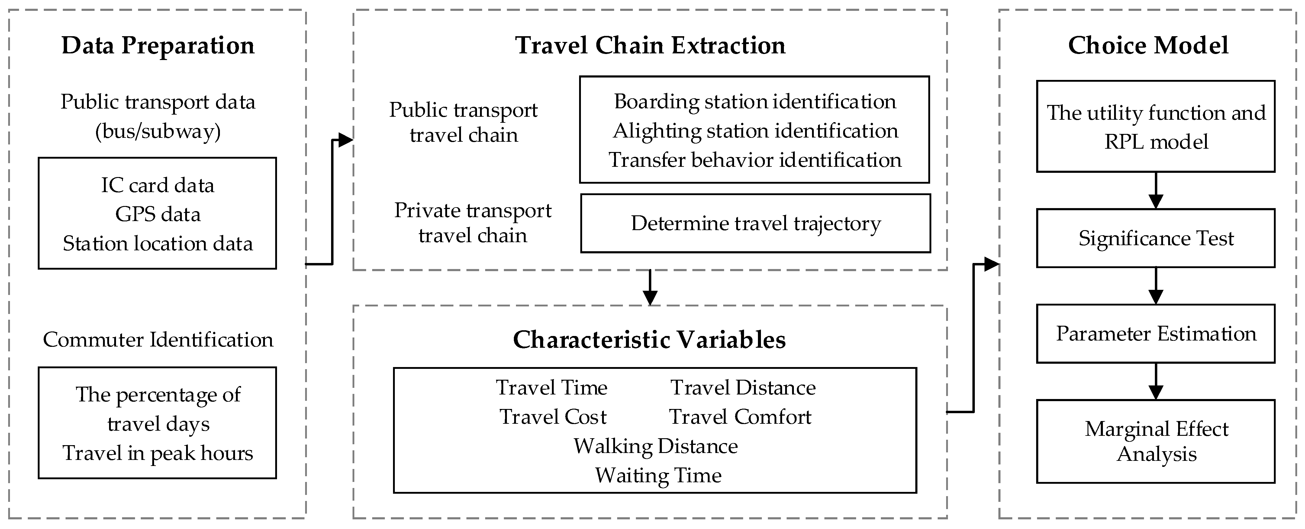
The fundamental assumption of the proposed model is that commuters have complete knowledge of the travel characteristics of each mode of transportation and will select the one that provides the greatest utility. The algorithm consists of three steps: First, the travel chain of all modes, including public transport (PT) and private transport (PC), is extracted. Second, based on the travel chain, the characteristics variables are analyzed and calculated. The final step entails constructing a multi-mode choice model for commuters using the RPL model and estimating its parameters using random utility maximization theory. The methodology framework is shown in Figure 5.

3. Travel Chain Extraction

The travel chain describes a traveler’s entire journey from the origin to multiple destinations and back to the origin. Generally speaking, a typical passenger travel chain consists of origin stations, origin lines, transfer stations, transfer lines, and destination stations. Therefore, a complete passenger’s travel chain will be discussed in terms of the following three components: boarding station, alighting station, and transfer behavior.

3.1. Boarding Station Identification

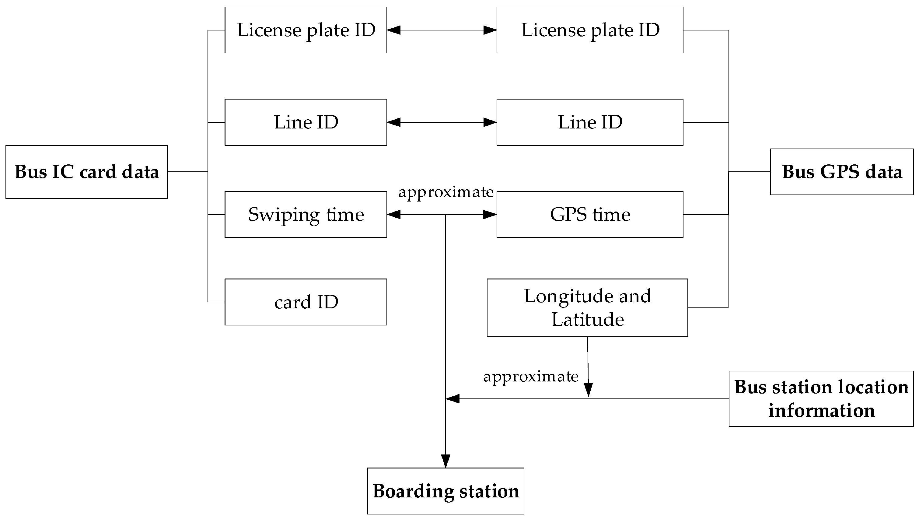
Identification of the boarding station is the first step in travel chain extraction. The data on the subway IC card include the boarding time and station, so additional analysis is unnecessary. However, for bus data, the boarding station falls short. Figure 6 depicts the boarding station identification process. First, the latitude and longitude of the boarding station can be deduced by comparing the same attributes (license plate number, line ID, and time) in the IC card and GPS data. Then, the closest station on the bus line is located to serve as the boarding location. Significantly, the time difference between card swiping and bus arrival is set to no more than three minutes in order to increase the matching success rate [35].

3.2. Alighting Station Identification

Passengers must swipe a card upon entering and exiting the subway station in order to accurately determine the alighting station based on travel records and station location data. However, the current bus fare system in China is primarily based on a single-ticket system, and IC cards do not contain information about the alighting station; therefore, it is necessary to confirm the alighting station. Several fundamental rules regarding travel logs for the same day are defined:
  • The passenger’s final destination is close to the origin of his or her first trip.
  • For consecutive trips of a passenger, the destination of the last trip is often close to the origin of the next trip.
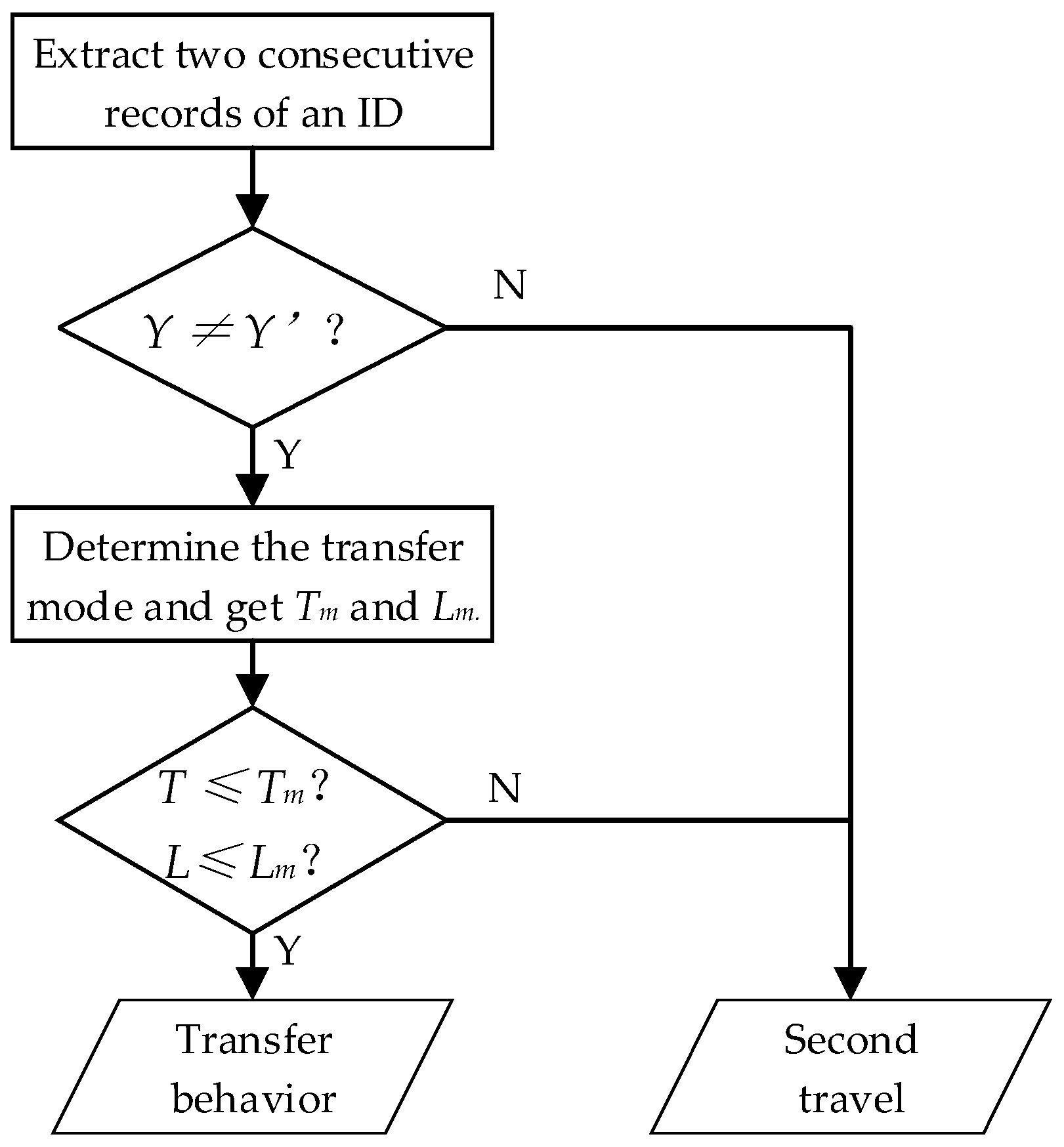
  • For two consecutive travel records of a passenger, the lines are Y and Y , respectively. If Y = Y and the running directions are opposite, their origins are each other’s destinations.
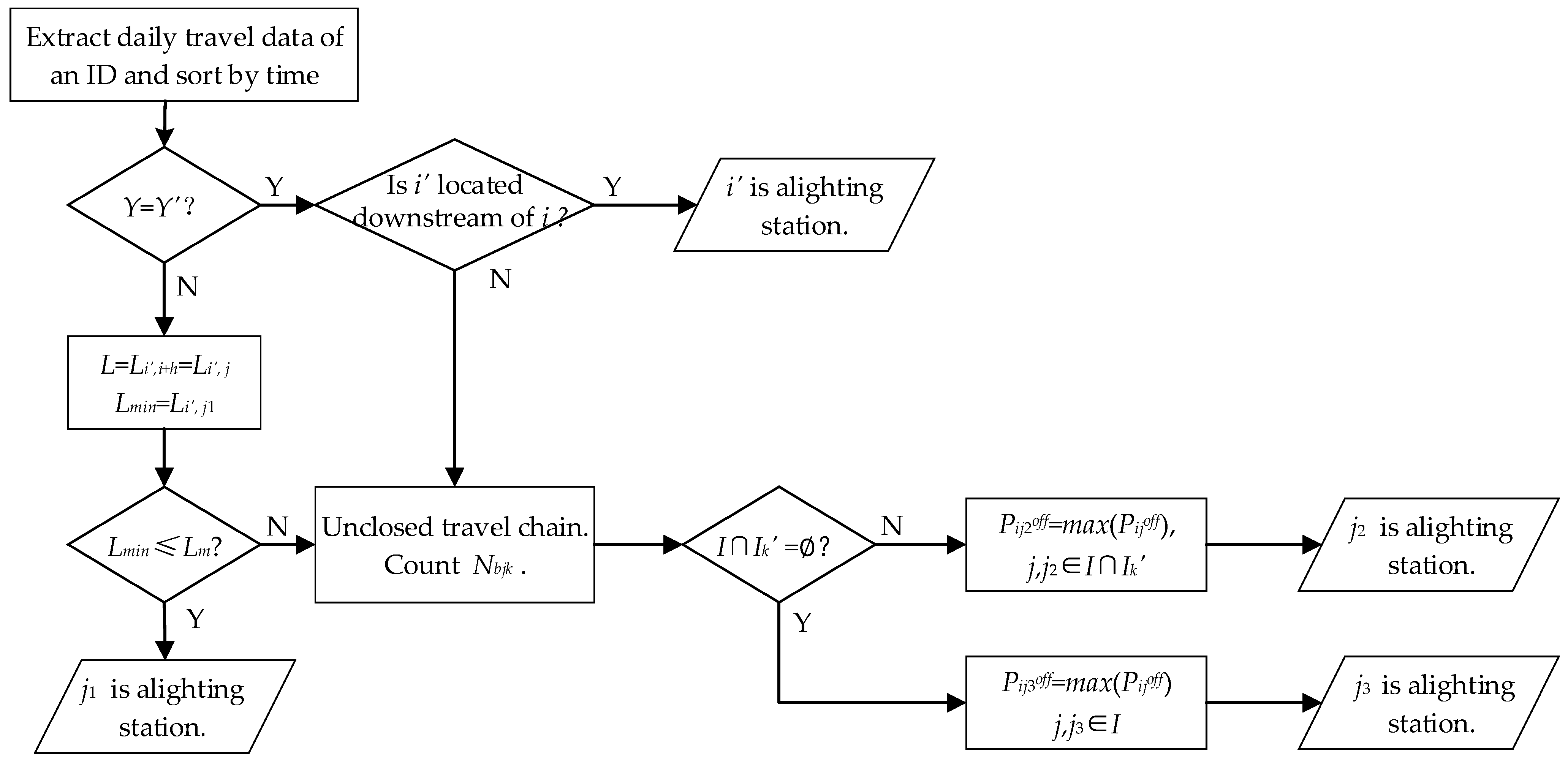
The alighting station of the closed travel chains can be easily identified using the above rules. For unclosed travel chains, however, it is difficult to confirm the alighting station; so, a method for calculating P i j o f f is proposed, which is represented as the probability of alighting at station j from station i, and the algorithm is detailed as follows:
(1) The card swiping times is N b , and that of passenger k at station j is represented as N b j k . The set of the downstream stations is I, and the set of stations where passenger k has boarded is I k .
(2) If I     I k , the passenger will get off at the station where he has boarded the most frequently, then P i j o f f is expressed as
P i j o f f = N b j k N b j k   ,   i < j   and   j I I k
(3) If I     I k = , the alighting station can be analyzed based on the passengers’ bus travel rules. When traveling by bus, the number of stations they pass through is primarily concentrated in a certain range, and the probability of alighting is greatest when a certain threshold is reached. Above or below this threshold, the probability decreases. Typically, the probability of a passenger alighting follows a Poisson distribution with the number of stations they pass through [42], which can be expressed as Equation (2). Since passengers transit between 1 and n − 1 (n is the number of stations on the line) stations in reality, P i j o f f * is therefore normalized as Equation (3):
P i j o f f * = e λ   ×   λ ( j i )   j i   ! ,   i < j   and   j I
P i j o f f = e λ   ×   λ ( j i )   j i   ! / i = 1 n 1 e λ   ×   λ ( j i )   j i   ! ,   i < j   and   j I  
where λ is the average number of stations passed by passengers on a bus line, which varies with different lines, setting λ = n     i if the number of downstream stations is less than λ.
(4) It is determined that the station j with the highest probability P i j o f f is the alighting station. Specifically, if two or more stations have identical maximum probabilities, the station closest to station i will be selected.
The complete description for this algorithm is shown in Figure 7.

3.3. Transfer Behavior Identification

The purpose of a passenger’s transfer behavior is to switch to a different line enroute and ultimately reach their destination. Figure 8 illustrates a simple example of a single change. Tv1 and Tv2 are the in-car times; Tw and WDw are the walking time and distance during the transfer; Td is the transfer waiting time. Two travel records can be generated due to the transfer with two card swipes, and it can also be obtained through the second travel; therefore, it is necessary to identify some distinguishing characteristics between the two behaviors.
As depicted in Figure 8, if the dwell time at a transfer station or the distance between two stations exceeds predetermined criteria, the behavior of transferring to a different line will be considered a separate trip. The time threshold T m and distance threshold L m are, therefore, defined as indicators (the subscript m represents the transfer mode). Moreover, T m is determined primarily by walking time and waiting time, and is expressed as T m = T w m a x + T d m a x . Due to the unique characteristics of transportation modes, T m and L m   could be valued differently.
  • B-B: bus-to-bus
Significant correlation exists between L B B and the maximum distance between adjacent bus stations. L B B   is typically set at 500 m in the central urban area and 700 m in the suburbs. Pedestrian walking speed is approximately 1.2 m/s, and the maximum walking distance is equivalent to L B B ; therefore, T w _ B B can be calculated as T w _ B B = L B B v p e d e s t r i a n , which is, respectively, 6.9 and 9.7 min in the major urban and suburban areas. T d _ B B is the maximum time interval between bus departures.
  • B-S and S-B: bus-to-subway and subway-to-bus
According to studies, the maximum distance passengers are willing to walk to reach subway stations is 770 m, so L B S   =   L S B   =   770   m and T w _ B S = T w _ S B   = 10.7   min . Meanwhile, T d _ B S is the maximum departure time interval for the subway, and T d _ S B represents the bus.
  • S-S: subway-to-subway
In this mode, the transfer time and distance can be disregarded because only two records at the origin and destination are stored, and the journey is regarded as identical.
In the research region, the maximum bus departure intervals in urban and suburban areas are 10 and 15 min, respectively, during peak hours and 15 and 30 min, respectively, during off-peak hours. The value for the subway is between 7.4 and 10.5 min. Table 2 displays the values of T m and L m for various transfer modes.
Figure 9 provides a comprehensive description of transfer behavior identification based on the preceding definition. First, the passenger’s daily travel records are sorted by time, and then the time difference between alighting time at stage k and boarding time at stage k + 1 is calculated using T   =   t k + 1   o n     t k   o f f . L is approximated by the Euclidean distance between the corresponding stations at time t k + 1   o n and   t k   o f f . If T     T m and L   L m , then the two records are defined as the transfer behavior in an identical travel.

3.4. Accuracy Validation

To examine the accuracy of the data and verify the efficacy of the data process, a test based on station passenger flow is conducted.
253,034 travel chains can be recognized by identifying the boarding, alighting, and transfer stations. Table 3 displays the travel chain information for a commuter with ID 2660000000556150, which includes card ID; boarding and alighting time, line, and station; and travel stage and mode. In addition, passengers boarding and alighting at each station can be tallied, and the feasibility of the extraction method is evaluated based on the criterion that the passenger flow at each station remains balanced over time.
Due to the round trips of passengers, the departures t p i and arrivals t a i at station i are generally equal [42], i.e., t p i   =   t a i . Nonetheless, the variety of travel plans enables passengers to make diverse travel decisions, which leads to bias, and the equation is rewritten as Equation (4). To determine the degree of correlation between t p i and t a i , correlation coefficient R * is introduced and its calculation process is shown in Equation (5).
t p i   =   a   ×   t a i + b
R * = [ ( t p i t p ¯ )   ×   ( t a i   t a ¯ ) ] ( t p i   t p ¯ )   ×   ( t a i t a ¯ )
where t p ¯ and t a ¯ are the average of t p i and t a i . When a 1 ,   b 0   and   R * 1 , the departures and arrivals of stations tend to balance, and the correlation becomes stronger.
t p i and t a i are counted and substituted into the preceding equation, and a and b are then estimated using the least squares method. The calculated results are a = 0.9793, b = 0.3509, and R * = 0.92, which indicates that departures and arrivals are roughly balanced, meet the accuracy requirements of station identification, and reflect the effectiveness and viability of the travel chain extraction method utilized in this paper.
It is difficult to obtain private traffic data, and license plate recognition (LPR) and taxi GPS data cannot be linked to specific individuals. However, PT and PC are interchangeable, so if commuters do not take PT, they will be assumed to have chosen PC. It is assumed that commuters do not request time off or travel for business during the study period, and that their residence is the origin and destination of their daily commute. Linking the travel chain of public transportation by time may result in the following situations:
(1) All public transportation travel chains within a 24-h period form a continuous chain; commuters do not choose PC travel.
(2) All public transportation travel chains within a single day cannot form a closed chain; a break exists. If a commuter takes a taxi to work and a bus home, the break is from home to workplace. Therefore, the number of breaks represents the number of travel chains by PC.
(3) Commuters who have not swiped their IC card in a few days will travel via PT. Additionally, the number of travel chains by PC can be expressed as the number of daily travel chains made by the commuters most frequently.
Following the preceding discussion, it is possible to calculate the number of travel chains by PT and PC, which are, respectively, 253,034 and 52,286, resulting in respective share rates of 82.87 and 17.13%.

4. Characteristic Variables for Choice Model

In existing literature, travel time, distance, and cost are frequently used to construct choice models [43,44]. In the meantime, Ashalatha notes that walking distance and wait time have a substantial impact on commuters’ mode choice [5]. Other than the attributes of the mode, travelers’ perceptions of the travel environment, such as comfort, cannot be ignored [45,46]. However, it is difficult to directly calculate travel comfort, so the passenger loading factor will be implemented. In this paper, therefore, travel time, distance, cost, comfort, walking distance, and waiting time are chosen as influential factors; the definitions and calculations are provided below.

4.1. Travel Time (TT) and Travel Distance (TD)

  • Public transport
Travel time can be directly calculated from the first boarding time t 1   o n and the last alighting time t s   o f f in an identical travel chain, expressed as T T P T   =   t s   o f f t 1   o n .
A coefficient   r i is introduced to correct errors caused by the road’s curvature, which represents the ratio of the actual distance l i of bus line i to its Euclidean distance d i ; namely, r i = l i / d i . Generally, if d i < 1 km, l i = 2   ×   d i ; otherwise, l i = d i . Consequently, T D P T can be calculated as follows:
T D P T   = k = 1 s ( r k   ×   d ( X k   o n ,   X k   o f f ) )
where X k   o n and X k   o f f are the boarding station and alighting station at stage k, k = 1,2, …, s; d ( X k   o n ,   X k   o f f ) is the Euclidean distance between X k   o n and X k   o f f .
  • Private transport
Through the investigation of road vehicles, it is found that buses and automobiles with comparable entry times on the same road face similar traffic conditions, so their traveling time and average speed are basically the same. The buses mentioned here do not have their stops on this road. Although PC’s travel time cannot be directly calculated, the route can be divided into several segments, and the driving of PC on this route is viewed as the driving of multiple buses on these segments. Thus, the travel time and distance of PC can be obtained, and the special steps are as follows.
The route between origin and destination is divided into N sections, i.e., l 1 , l 2 , , l N . For section l 1 , the average speed of private cars is approximately equal to that of bus A, i.e., v 1 ¯ = v A ¯ ; therefore, the driving time of private cars on section l 1 can be expressed as T 1 = l 1 / v 1 ¯ = l 1 / v A ¯ . In other sections, the same calculation is applied. The total travel time and distance for private cars can be expressed as:
T T P C = n = 1 N T n
T D P C = n = 1 N l n
In addition, this paper uses the k-shortest path algorithm to determine the optimal driving route, with k set to 3 in accordance with navigation search rules. The route with the shortest travel time will be chosen as the driving path for private cars, which is also the PC travel chain for this commuter.

4.2. Travel Cost (TC)

  • Public transport
Using the transaction amount recorded by bus/subway IC card data and the information extracted from the passenger travel chain, it is simple to calculate the cost of public transportation.
  • Private transport
Private transportation consists primarily of taxis and private cars. When commuters have cars, they are more willing to travel by private car than by taxi [47,48]; therefore, car ownership is an important factor to judge whether commuters choose taxis or private cars for private travel. This information is absent from the existing content, but it is possible to estimate the number of owners by analyzing the probability of car ownership, which will be used to mark the attribute of commuters’ car ownership. There are approximately 1.24 million residents and 0.36 million cars in the study area, so the probability of ownership is approximately 29%; or, 29% of people have cars. Therefore, 1513 commuters are selected at random, identified as car owners, and assigned to drive for personal travel.
T C c a r and T C t a x i represent private car and taxi travel cost. T C c a r is determined by travel distance ( T D c a r ), fuel consumption per kilometer (FCK), and fuel price (FP), i.e., T C c a r = T D c a r   ×   F C K   ×   F P . FCK = 0.0685 L/km [49] and FP = 7.025 CNY/L through the investigation. T C t a x i has special charging rules and is primarily associated with travel distance; the calculation is shown below. In particular, for night travel (from 22:00 to 5:00 the next day), the mileage fee increases by 0.4 CNY/km.
T C t a x i = α 0 , x     3   km α 0 + 3 x α 1 d x , 3   km   <   x     10   km α 0 + 3 10 α 1 d x + 10 x α 2 d x , 10   km   <   x     35   km α 0 + 3 10 α 1 d x + 10 35 α 2 d x 35 x α 3 d x , x   >   35   km
where x represents the travel distance; α 0 is the flag-fall price, which is CNY 9 if x     3   km ; and α 1 , α 2 , and α 3 represent mileage fee for different distance ranges. α 1 = 1.4 CNY/km, α 2 = 1.5   ×   α 1 ,   α 3 = 2   ×   α 1 .

4.3. Travel Comfort (CF)

  • Public transport
The passenger load factor LR is defined as the ratio of the number of actual passengers on a bus to its maximum capacity RPC, which is used to calculate the level of public travel comfort [50].
L R k = A P C k R P C
A P C k = j = 1 k 1 ( N a j N b j )
C F P T = 1 L R ¯ = 1 k I p L R k N p
N a j and N b j represent the number of passengers boarding and alighting at station j, while A P C k   is the actual number of passengers on the bus at station k. Setting station k I p , I p represents the set of stations which the passenger passes through, and its size is N p .
  • Private transport
This paper assigns PC a value of 1 for travel comfort, i.e., C F P C = 1 , because private cars and taxis ensure that every passenger has a seat and their environment is significantly more pleasant than that of public transportation.

4.4. Walking Distance (WD)

  • Public transport
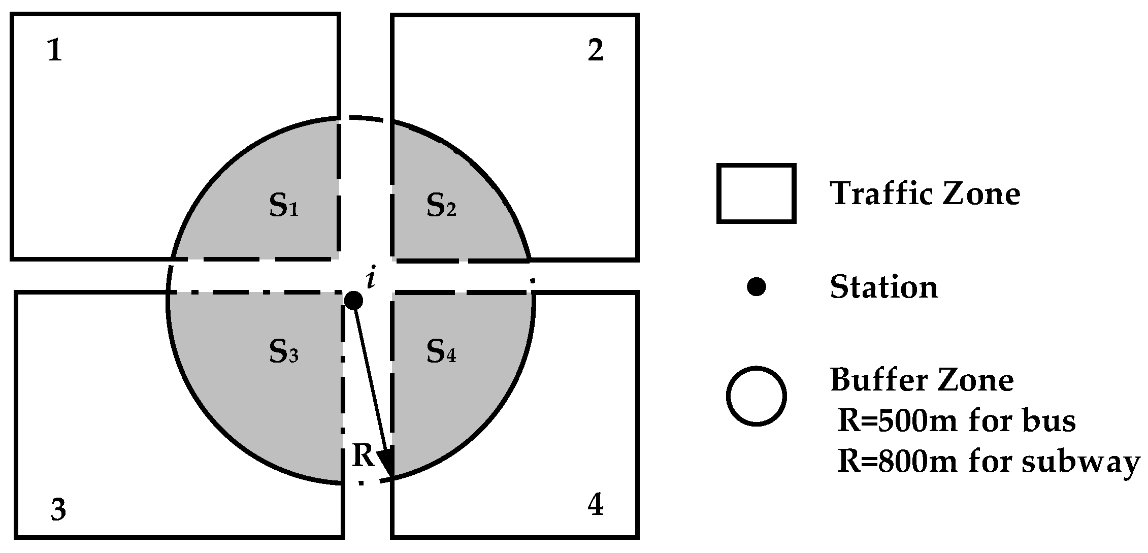
Generally speaking, this characteristic value refers to the transfer walking distance ( W D t r ) and the distance walking to the original station ( W D s t ). Due to the facts that the extracted travel chain uses the station as the node, a station may serve multiple traffic zones (See Figure 10), and the distance from different zones to the same station varies, it is necessary to analyze the origin of passengers.
In this paper, the spatial relationship between the station and the surrounding traffic zones serves as a metaphor for the relationship between their passengers, and the proportion of trips from the station to all nearby zones is defined as being equal to the proportion of overlapping area between the buffer zone and traffic zones. Therefore, the number of passengers of traffic zone j departing from station i is represented as O i j , and the calculation is expressed as follows:
O i j = S i j k = 1 K S i k   ×   q i
where S i j is the overlapping area between the buffer zone of station i and traffic zone j; q i is the number of passengers departing from station i; and K is the number of the surrounding traffic zones.
Passengers at station i are randomly selected based on the number of passengers from each traffic zone, and the corresponding traffic zone is labeled as their origin. W D s t is thus defined as the distance from the centroid of the origin X 0 to the first boarding station X 1   o n . W D t r is the sum of the walking distance of all transfer stages; therefore, the calculation process of W D P T is calculated as follows.
W D P T = W D s t + W D t r
W D s t = d ( X 0 ,   X 1   o n )
W D t r = c W D w   = c d ( X k   o f f ,   X k + 1   o n )
where X k ,   X k + 1 represent the adjacent bus stations for each transfer, X k   o f f is the alighting station at stage k, and X k + 1   o n is the boarding station at stage k + 1; c is the transfer time.
  • Private transport
Taxi passengers must walk to the nearby roadside in order to hail a cab. Drivers of private vehicles must walk to their parking spot, which may be in a parking lot or along the road outside the zone. This paper describes the walking distance of these two modes uniformly as the straight-line distance from the origin’s centroid X 0 to its nearest road W m , i.e., W D P C =   d   ( X 0 , W m ) .

4.5. Waiting Time (WT)

  • Public transport
The waiting time for PT can be broken down into starting station waiting time W T s t and transfer station waiting time W T t r . Several studies indicate a correlation between station wait times and the distribution of passenger and vehicle arrival times. If passengers’ arrival time is subject to uniform distribution and the departure time interval of vehicles is constant, W T s t is half of the departure time interval T y of line y [51], i.e., W T s t   =   T y / 2 . Since the transfer time comprises transfer waiting time and transfer walking time, W T t r is written as
W T t r = c ( T d ) = c ( t k + 1   o n t k   o f f W D w v p e d e s t r i a n )
where t k + 1   o n is the boarding time at stage k + 1, and t k   o f f is the alighting time at stage k; W D w is transfer walking distance.
  • Private transport
When passengers travel by private car or taxi, they can leave at any time with little need to wait; therefore, W T P C   =   0 .

5. Parameter Calibration for RPL Model

5.1. The Utility Function and RPL Model

The logit model is typically based on random utility maximization theory, which assumes that travelers are aware of all available options and choose the one that provides the greatest utility. The utility of traveler i choosing alternative j typically consists of deterministic component V i j and random component ε i j [52]. V i j is defined as a linear combination of observable variables and their coefficient β (see Equation (18)). Then, the probability that alternative j is chosen by traveler i is given by Equation (19) [53], and in this paper, alternatives include both public and private transportation.
V i j = β T T × T T i j + β T D × T D i j + β T C × T C i j + β C F × C F i j + β W D × W D i j + β W T × W T i j + A S C j
Prob   y i = j   = exp ( V i j ) j exp ( V i j )
where ASC is the alternative specific constant that reflects the effect of alternatives themselves on utility. In this study, PC is set as the reference alternative; therefore, A S C P C = 0 [54] and A S C P C represents the relative utility between PT and PC.
Different from other logit models, RPL model sets some parameters to be random and follow a distribution, and β i is written as
β i   =   β 0   +   σ     ×     ν i
where β 0 is the population mean; σ is the standard deviation; and ν i   represents the heterogeneity parameter of individual i, which is a vector composed of M random variables with mean zero and standard deviation one, M being the number of individuals i.

5.2. Significance Test of Characteristic Variables

Economic development, road network, and infrastructure construction make the same factors have varying effects on the travel of residents in different regions, and the identification of these factors will have a direct bearing on the establishment of a utility function. Therefore, prior to parameter estimation, it is necessary to determine if each factor has a significant impact on the travel preferences of residents in this region.
The travel preference of each passenger with the characteristics of each travel plan is linked, and then this information is used as the model’s input. The max-minimum standardization method is applied to these data in order to avoid the effect of large data gaps between different characteristic variables. Then, the MNL model is estimated using NLOGIT to determine the initial value of each parameter of the RPL model, and the results can be used to assess the significance of each parameter [55]. Due to the size of the sample, one thousand Halton sequences are used to estimate the parameters to prevent the model from failing to converge due to insufficient sampling times. The estimated results are displayed in Table 4.
Principally, the z test and p value are used to evaluate the significance level of characteristic variables. When p is less than 0.05 and z is greater than 1.96, variables are considered to have a significant impact on the selection outcomes. According to Table 4, the values of p for all variables are less than 0.05, and the absolute values of z are all greater than 1.96, indicating that these factors have a significant impact on travel mode selection and that Equation (18) is valid.

5.3. Parameter Estimation for RPL Model

Some RPL model parameters are distributed, and their coefficients can be expressed as Equation (20). Given that few parameters are used in this paper, the enumeration method is used to generate random values for some or all of them before parameter calibration. In general, it is assumed that random coefficients follow a normal distribution, and other distributions are considered only when the running results are not satisfied [56,57]. The characteristic attributes of each alternative and mode option are input, and 1000 iterations of Halton sequence sampling are utilized. The parameters for each case are estimated, and the results are evaluated using a significance threshold. WD is subsequently identified as a random parameter, and its coefficient can be expressed as: β W D i = β 0 W D + σ W D ν W D i . The final results are displayed in Table 5.
Pseudo R2 is 0.4330 in the RPL model and 0.4128 in the MNL model, indicating that the RPL model is superior to the MNL model and better describes commuters’ travel choices. Table 5’s parameter calibration results comply with the significance judgment rule (p < 0.05 and z > 1.96), so the deterministic component of traveler i choosing alternative j can be expressed as:
V P T = ( 8.127   +   4.73   ×   ν W D )   ×   W D P T 0.977   ×   T T P T 7.604   ×   T D P T 2.55   ×   T C P T + 6.609   ×   C F P T 1.279   ×   W T P T + 4.401
V P C = ( 8.127   +   4.73   ×   ν W D )   ×   W D P C 0.977   ×   T T P C 7.604   ×   T D P C 2.55   ×   T C P C + 6.609   ×   C F P C 1.279   ×   W T P C
Consistent with the actual situation, the coefficient of CF is positive, indicating that travel comfort has a positive impact on travelers’ utility, while others have a negative impact on travelers’ utility. WD, TD, and CF have greater coefficients, indicating that they have a greater influence on the choice of travel mode than other variables. Additionally, WD is a random parameter with a coefficient that follows the normal distribution of N (−8.127, 4.7302). The probability of β W D < 0 is calculated using a normal distribution calculator as: p ( β W D < 0) = 0.9573. It is interpreted that if the walking distance of a mode of transportation increases, 95.73% of commuters have a lower probability of choosing this travel mode, while 4.27% of them have a higher probability of choosing it, reflecting the heterogeneity among commuters. The value of A S C P T is 4.401, which means that the utility difference between PT and PC is 4.401, and indicates that commuters prefer to travel by PT regardless of other influencing factors.

5.4. Marginal Effect Analysis

The logit model is a nonlinear model, so the coefficient value of each parameter cannot represent its degree of influence on travel mode selection; therefore, marginal effect analysis must be performed on the model. Marginal effect represents the change in the choice probability P j of alternative j caused by a one-unit change in the variable X j k ( X k includes TT, TD, TC, CF, WT, and WD) that is denoted by M X j k . It is calculated using the probability weighted sample enumeration (PWSE) method [55], which computes the marginal effect M X i j k of individual i and then weights it with the choice probability P i j . The calculation is displayed in Equations (23) and (24). Table 6 provides the results. By analyzing the degree of influence of parameters on the probability of different modes of transportation, more reasonable measures are proposed to help managers achieve their goals.
M X j k = i = 1 M ( P i j   ×   M X i j k ) / i = 1 M P i j
M X i j k = P i j X i j k = 1 P i j   ×   β j k
Changes in Table 6’s TD, CF, and WD have a significant impact on the probability of selecting PT. Long distances, overcrowding, or stations located too far from the origin may discourage commuters from continuing to use PT. It also demonstrates that changes in TD, TC, and CF have a significant effect on the probability that PC will be selected. Commuters will utilize more PT if comfort deteriorates or if travel expenses and distance increase.
Given that the sum of the choice probabilities must equal 1, the total marginal effect of each variable is 0. In the case of TC, when the cost of PT increases by one unit, the probability of selecting PT decreases by 0.003 and the probability of selecting PC rises by 0.003 when all other conditions remain unchanged. The probability of selecting PC decreases by 0.192 units for each unit increase in PC cost, while the probability of selecting PT increases by 0.192 units. Moreover, it was discovered that increasing the cost of PC has a greater effect on encouraging travelers to choose PT than reducing the cost of PT. Consequently, administrators can increase the travel cost of private transport, such as by adjusting gas prices or taxi fares, to encourage more commuters to use public transportation.

6. Conclusions and Discussion

This paper identifies the boarding stations, alighting stations, and transfer behaviors of commuters based on smart card data, GPS data, and station location data of urban public transportation, and extracts a complete public transportation travel chain. Then, considering the travel characteristics of commuters (round-trip and closed-off), private travel chains are obtained based on the origin and destination of each travel stage. The quality of every station’s passenger flow to maintain equilibrium over time is observed. By analyzing the station’s departures and arrivals, the feasibility and efficacy of the travel chain extraction method have been demonstrated. The results of parameter calibration indicate that travel time, distance, comfort, cost, walking distance, and waiting time have a significant impact on mode selection. Walking distance is the most influential variable, and its coefficient follows the normal distribution of N (−8.127, 4.7302), which reflects the preference heterogeneity of travelers. In addition, this paper analyzes the marginal effect of each variable on travel mode selection, i.e., the degree to which the probability of selecting each transport mode is influenced by changes in various factors. These findings can be used as a basis for adjusting the structure of the urban transportation system.
This paper is also a novel effort to replace traditional survey data with the travel characteristic value extracted from the travel chain, and it has been successful. In light of the findings of this study, government agencies can take the following steps to alleviate urban traffic congestion and encourage more urban residents to use public transportation: Increase the costs of private transportation in an appropriate manner, such as by modifying fuel prices and taxi fares, etc. Optimize the layout of public transport platforms and lines, add new platforms, or relocate existing platforms in densely populated areas so that residents can more easily utilize public transportation. During peak travel times, the frequency of public transportation can be reduced to prevent overcrowding caused by an excessive number of passengers in the bus. In addition, attention must be paid to the cleanliness of the vehicle in order to maintain a clean travel environment and provide passengers with a better travel experience.
This paper’s limitations primarily stem from two aspects. On the one hand, the influence factors focus primarily on the characteristics of the mode of transport, ignoring the influence of individual characteristics such as socioeconomic attributes and psychological factors. In the future, residents’ surveys and other methods can be used to enrich the detailed information of travelers and analyze the influence of individual characteristics on travel selection. On the other hand, this paper discusses commuters’ choice between public and private transportation, but does not further categorize each mode. Take public transportation as an example; there are various travel combinations, such as bus-only, bus-and-subway, and subway-only. Despite the fact that they are all forms of public transportation, travelers will make different decisions depending on the circumstances. Subsequent research may subdivide each mode and investigate the multi-modal selection behavior of travelers.

Author Contributions

Conceptualization, L.C. and Y.Z.; methodology, L.C. and Y.Z.; software, Y.Z. and X.Y.; validation, Y.Z.; formal analysis, L.C. and Y.Z.; investigation, Y.Z. and X.Y.; resources, L.C.; data curation, Y.Z. and X.Y.; writing—original draft preparation, Y.Z.; writing—review and editing, L.C. and Z.L.; supervision, L.C. and Z.L.; project administration, L.C.; funding acquisition, L.C. All authors have read and agreed to the published version of the manuscript.

Funding

This research was funded by Ministry of education of Humanities and Social Science project (19YJCZH007).

Institutional Review Board Statement

Not applicable.

Informed Consent Statement

Not applicable.

Data Availability Statement

The data can only be shared internally within the institute where the corresponding author works.

Conflicts of Interest

The authors declare no conflict of interest.

References

  1. Zeng, N.; Wang, Z. Analysis of Beijing-Guangzhou High-Speed Railway Competitiveness Based on Generalized Travel Cost Model. IOP Conf. Ser. Earth. Environ. Sci 2020, 587, 12099. [Google Scholar] [CrossRef]
  2. Sun, L.; Gao, Z. An equilibrium model for urban transit assignment based on game theory. Eur. J. Oper. Res. 2007, 181, 305–314. [Google Scholar] [CrossRef]
  3. Hasnine, M.S.; Lin, T.; Weiss, A.; Habib, K.N. Determinants of travel mode choices of post-secondary students in a large metropolitan area: The case of the city of Toronto. J. Transp. Geogr. 2018, 70, 161–171. [Google Scholar] [CrossRef]
  4. Tang, X.; Wang, D.; Sun, Y.; Chen, M.; Waygood, E.O.D. Choice behavior of tourism destination and travel mode: A case study of local residents in Hangzhou, China. J. Transp. Geogr. 2020, 89, 102895. [Google Scholar] [CrossRef]
  5. Ashalatha, R.; Manju, V.S.; Zacharia, A.B. Mode Choice Behavior of Commuters in Thiruvananthapuram City. J. Transp. Eng-Asce 2013, 139, 494–502. [Google Scholar] [CrossRef]
  6. Witchayaphong, P.; Pravinvongvuth, S.; Kanitpong, K.; Sano, K.; Horpibulsuk, S. Influential Factors Affecting Travelers’ Mode Choice Behavior on Mass Transit in Bangkok, Thailand. Sustainability 2020, 12, 9522. [Google Scholar] [CrossRef]
  7. Ha, J.; Lee, S.; Ko, J. Unraveling the impact of travel time, cost, and transit burdens on commute mode choice for different income and age groups. Transp. Res. Part A Policy Pract. 2020, 141, 147–166. [Google Scholar] [CrossRef]
  8. Habib, K.N.; Mahmoud, M.S.; Coleman, J. Effect of parking charges at transit stations on park-and-ride mode choice: Lessons learned from stated preference survey in Greater Vancouver, Canada. Transport. Res. Rec. 2013, 2351, 163–170. [Google Scholar] [CrossRef]
  9. Albert, G.; Mahalel, D. Congestion tolls and parking fees: A comparison of the potential effect on travel behavior. Transp. Policy. 2006, 13, 496–502. [Google Scholar] [CrossRef]
  10. Link, H. Is car drivers’ response to congestion charging schemes based on the correct perception of price signals? Transp. Res. Part A Policy Pract. 2015, 71, 96–109. [Google Scholar] [CrossRef]
  11. Andersson, D.; Nässén, J. The Gothenburg congestion charge scheme: A pre–post analysis of commuting behavior and travel satisfaction. J. Transp. Geogr. 2016, 52, 82–89. [Google Scholar] [CrossRef]
  12. Ku, D.; Um, J.; Byon, Y.; Kim, J.; Lee, S. Changes in Passengers’ Travel Behavior Due to COVID-19. Sustainability 2021, 13, 7974. [Google Scholar] [CrossRef]
  13. Bhaduri, E.; Manoj, B.S.; Wadud, Z.; Goswami, A.K.; Choudhury, C.F. Modelling the effects of COVID-19 on travel mode choice behaviour in India. Transp. Res. Interdiscip. Perspect. 2020, 8, 100273. [Google Scholar] [CrossRef]
  14. Hyland, M.; Frei, C.; Frei, A.; Mahmassani, H.S. Riders on the storm: Exploring weather and seasonality effects on commute mode choice in Chicago. Travel. Behave. Soc. 2018, 13, 44–60. [Google Scholar] [CrossRef]
  15. Böcker, L.; Priya Uteng, T.; Liu, C.; Dijst, M. Weather and daily mobility in international perspective: A cross-comparison of Dutch, Norwegian and Swedish city regions. Transp. Res. Part D Transp. Environ. 2019, 77, 491–505. [Google Scholar] [CrossRef]
  16. Keyes, A.K.M.; Crawford-Brown, D. The changing influences on commuting mode choice in urban England under Peak Car: A discrete choice modelling approach. Transp. Res. Part F Traffic. Psychol. Behav. 2018, 58, 167–176. [Google Scholar] [CrossRef]
  17. Benson, A.R.; Kumar, R.; Tomkins, A. On the Relevance of Irrelevant Alternatives. In Proceedings of the 25th International Conference on World Wide Web, Montréal, QC, Canada, 11–15 April 2016; pp. 963–973. [Google Scholar]
  18. Yang, L.; Zheng, G.; Zhu, X. Cross-nested logit model for the joint choice of residential location, travel mode, and departure time. Habitat. Int. 2013, 38, 157–166. [Google Scholar] [CrossRef]
  19. Sarrias, M.; Daziano, R. Multinomial Logit Models with Continuous and Discrete Individual Heterogeneity in R: The gmnl Package. J. Stat. Softw. 2017, 79, 1–46. [Google Scholar] [CrossRef] [Green Version]
  20. Mcfadden, D.; Train, K. Mixed MNL models for discrete response. J. Appl. Econ. 2000, 15, 447–470. [Google Scholar]
  21. Regier, D.A.; Ryan, M.; Phimister, E.; Marra, C.A. Bayesian and classical estimation of mixed logit: An application to genetic testing. J. Health. Econ. 2009, 28, 598–610. [Google Scholar] [CrossRef]
  22. Fuhrer, J.C.; Moore, G.R.; Schuh, S.D. Estimating the linear-quadratic inventory model maximum likelihood versus generalized method of moments. J. Monet. Econ. 1995, 35, 115–157. [Google Scholar] [CrossRef]
  23. Train, K.E. Discrete Choice Methods with Simulation, 2nd ed.; Cambridge University Press: New York, NY, USA, 2009; ISBN 978-0-521-76655-5. [Google Scholar]
  24. Li, Y.; Yao, E.; Yang, Y.; Zhuang, H. Modeling the Tourism Travel Mode and Route Choice Behaviour Based on Nested Logit Model. In Proceedings of the 2020 IEEE 5th International Conference on Intelligent Transportation Engineering, Beijing, China, 11–13 September 2020; pp. 28–32. [Google Scholar]
  25. Ilahi, A.; Belgiawan, P.F.; Balac, M.; Axhausen, K.W. Understanding travel and mode choice with emerging modes; a pooled SP and RP model in Greater Jakarta, Indonesia. Transp. Res. Part A Policy Pract. 2021, 150, 398–422. [Google Scholar] [CrossRef]
  26. Otim, T.; Dörfer, L.; Ahmed, D.B.; Munoz Diaz, E. Modeling the Impact of Weather and Context Data on Transport Mode Choices: A Case Study of GPS Trajectories from Beijing. Sustainability 2022, 14, 6042. [Google Scholar] [CrossRef]
  27. Kang, H.; Scott, D.M. Exploring day-to-day variability in time use for household members. Transp. Res. Part A Policy Pract. 2010, 44, 609–619. [Google Scholar] [CrossRef]
  28. Xianyu, J.; Rasouli, S.; Timmermans, H.J.P. Analysis of variability in multi-day GPS imputed activity-travel diaries using multi-dimensional sequence alignment and panel effects regression models. Transportation 2017, 44, 533–553. [Google Scholar] [CrossRef]
  29. Huang, Y.; Gao, L.; Ni, A.; Liu, X. Analysis of travel mode choice and trip chain pattern relationships based on multi-day GPS data: A case study in Shanghai, China. J. Transp. Geogr. 2021, 93, 103070. [Google Scholar] [CrossRef]
  30. Faroqi, H.; Mesbah, M. Inferring trip purpose by clustering sequences of smart card records. Transp. Res. Part C Emerg. Technol. 2021, 127, 103131. [Google Scholar] [CrossRef]
  31. Kusakabe, T.; Asakura, Y. Behavioural data mining of transit smart card data: A data fusion approach. Transp. Res. Part C Emerg. Technol. 2014, 46, 179–191. [Google Scholar] [CrossRef]
  32. Ma, X.; Wu, Y.; Wang, Y.; Chen, F.; Liu, J. Mining smart card data for transit riders’ travel patterns. Transp. Res. Part C Emerg. Technol. 2013, 36, 1–12. [Google Scholar] [CrossRef]
  33. Kieu, L.; Bhaskar, A.; Chung, E. A modified Density-Based Scanning Algorithm with Noise for spatial travel pattern analysis from Smart Card AFC data. Transp. Res. Part C Emerg. Technol. 2015, 58, 193–207. [Google Scholar] [CrossRef]
  34. Huang, D.; Yu, J.; Shen, S.; Li, Z.; Zhao, L.; Gong, C. A Method for Bus OD Matrix Estimation Using Multisource Data. J. Adv. Transp. 2020, 2020, 1–13. [Google Scholar] [CrossRef]
  35. Cong, J.; Gao, L.; Juan, Z. Improved algorithms for trip-chain estimation using massive student behaviour data from urban transit systems. IET Intell. Transp. Sy 2019, 13, 435–442. [Google Scholar] [CrossRef]
  36. Ya, W.; Bowen, D.; Qiannan, R.; Xia, L. Travel Patterns Analysis of Urban Residents Using Automated Fare Collection System. Chinese. J. Electron. 2016, 1, 8. [Google Scholar] [CrossRef]
  37. Cheon, S.H.; Lee, C.; Shin, S. Data-driven stochastic transit assignment modeling using an automatic fare collection system. Transp. Res. Part C Emerg. Technol. 2019, 98, 239–254. [Google Scholar] [CrossRef]
  38. Yong, J.; Zheng, L.; Mao, X.; Tang, X.; Gao, A.; Liu, W. Mining metro commuting mobility patterns using massive smart card data. Phys. A 2021, 584, 126351. [Google Scholar] [CrossRef]
  39. Shao, S.; Lu, L.; Liu, H.; Xiao, L. Analyzing Jobs-Housing Spatial Relationship Based on Floating Car Data. In Proceedings of the 2018 5th International Conference on Information, Cybernetics, and Computational Social Systems (ICCSS), Hangzhou, Zhejiang, China, 16–19 August 2018; pp. 489–494. [Google Scholar]
  40. Fan, X.; Xu, C.; Tang, F.; Qi, J.; Liu, X.; Chen, L.; Wang, C. CommuteShare: A Ridesharing Service for Daily Commuters Using Cross-Domain Urban Big Data. In Proceedings of the 2018 IEEE International Conference on Web Services (ICWS), San Francisco, CA, USA, 2–7 July 2018; pp. 298–301. [Google Scholar]
  41. Mei, Z.; Ding, W.; Feng, C.; Shen, L. Identifying commuters based on random forest of smartcard data. IET Intell. Transp. Syst. 2020, 14, 207–212. [Google Scholar] [CrossRef]
  42. Liu, W.; Tan, Q.; Liu, L.; Hussein, A.; Abulkasim, H. Destination Estimation for Bus Passengers Based on Data Fusion. Math. Probl. Eng. 2020, 2020, 1–10. [Google Scholar] [CrossRef]
  43. Al-Salih, W.Q.; Esztergár-Kiss, D. Linking Mode Choice with Travel Behavior by Using Logit Model Based on Utility Function. Sustainability 2021, 13, 4332. [Google Scholar] [CrossRef]
  44. Bai, T.; Li, X.; Sun, Z. Effects of cost adjustment on travel mode choice: Analysis and comparison of different logit models. Transp. Res. Procedia 2017, 25, 2649–2659. [Google Scholar] [CrossRef]
  45. Paulssen, M.; Temme, D.; Vij, A.; Walker, J.L. Values, attitudes and travel behavior: A hierarchical latent variable mixed logit model of travel mode choice. Transportation 2014, 41, 873–888. [Google Scholar] [CrossRef] [Green Version]
  46. Shen, Q.; Chen, P.; Pan, H. Factors affecting car ownership and mode choice in rail transit-supported suburbs of a large Chinese city. Transp. Res. Part A Policy Pract. 2016, 94, 31–44. [Google Scholar] [CrossRef]
  47. Ma, S.; Yu, Z.; Liu, C. Nested Logit Joint Model of Travel Mode and Travel Time Choice for Urban Commuting Trips in Xi’an, China. J. Urban Plan Dev. 2020, 146, 4020020. [Google Scholar] [CrossRef]
  48. Li, W.; Feng, W.; Yuan, H. Multimode Traffic Travel Behavior Characteristics Analysis and Congestion Governance Research. J. Adv. Transp. 2020, 2020, 1–8. [Google Scholar] [CrossRef]
  49. Yang, Z.; Wang, B.; Jiao, K. Life cycle assessment of fuel cell, electric and internal combustion engine vehicles under different fuel scenarios and driving mileages in China. Energy 2020, 198, 117365. [Google Scholar] [CrossRef]
  50. Shen, X.; Feng, S. How public transport subsidy policies in China affect the average passenger load factor of a bus line. Res. Transp. Bus. Manag. 2020, 36, 100526. [Google Scholar] [CrossRef]
  51. Chen, W.; Li, Z.; Liu, C.; Ai, Y. A Deep Learning Model with Conv-LSTM Networks for Subway Passenger Congestion Delay Prediction. J. Adv. Transp. 2021, 2021, 1–10. [Google Scholar] [CrossRef]
  52. Bhat, C.R. A heteroscedastic extreme value model of intercity travel mode choice. Transp. Res. Part B Methodol. 1995, 29, 471–483. [Google Scholar] [CrossRef]
  53. Hensher, D.A.; Greene, W.H. The Mixed Logit model: The state of practice. Transportation 2003, 30, 133–176. [Google Scholar] [CrossRef]
  54. Cheng, H.; Yang, X. Random Parameter Nested Logit Model for Combined Departure Time and Route Choice. Int. J. Transp. Sci. Technol. 2015, 4, 93–105. [Google Scholar] [CrossRef] [Green Version]
  55. Hensher, D.; Rose, J.; Greene, W. Applied Choice Analysis, 2nd ed.; Cambridge University Press: Cambridge, UK, 2015; ISBN 978-1-107-46592-3. [Google Scholar]
  56. Mariel, P.; Meyerhoff, J. More Flexible Model or Simply More Effort? On the Use of Correlated Random Parameters in Applied Choice Studies. Ecol. Econ. 2018, 154, 419–429. [Google Scholar] [CrossRef]
  57. Zhao, X.; Yan, X.; Yu, A.; Van Hentenryck, P. Prediction and behavioral analysis of travel mode choice: A comparison of machine learning and logit models. Travel. Behav. Soc. 2020, 20, 22–35. [Google Scholar] [CrossRef]
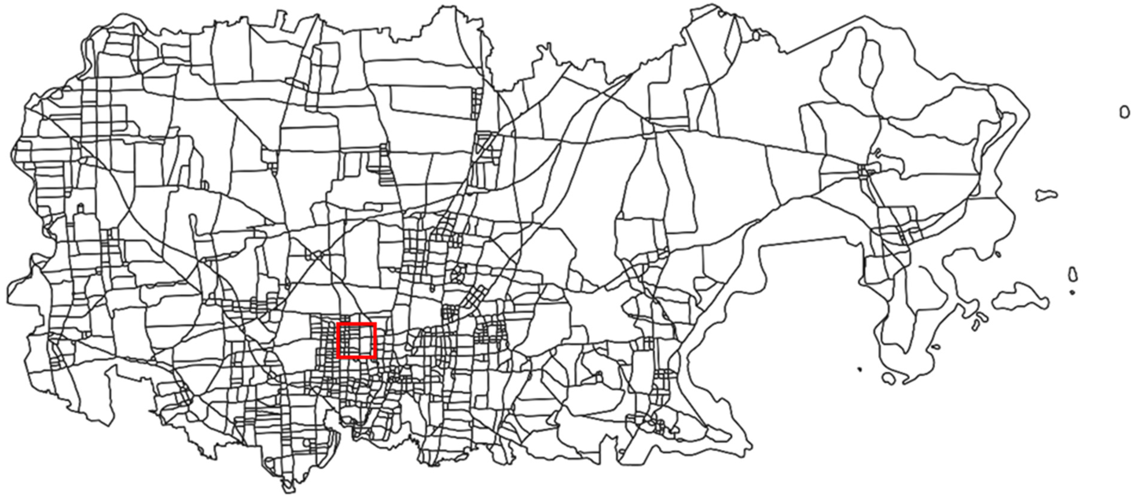
Figure 1. Traffic zone division.
Sustainability 14 15455 g001
Figure 2. The centroids of the traffic zones in the box selected in Figure 1.
Sustainability 14 15455 g002
Figure 3. Changes in daily traffic flow during the week.
Sustainability 14 15455 g003
Figure 4. Commuter identification process.
Sustainability 14 15455 g004
Figure 5. Methodology Framework.
Sustainability 14 15455 g005
Figure 6. Identification process for boarding station.
Sustainability 14 15455 g006
Figure 7. Alighting station identification process. L i , i + h is the Euclidean distance between station i and i + h, and i + h is the downstream station of i. L m is the distance threshold, whose value is shown in Table 1.
Sustainability 14 15455 g007
Figure 8. The description of a single change.
Sustainability 14 15455 g008
Figure 9. Identification process for transfer behavior.
Sustainability 14 15455 g009
Figure 10. Spatial relationship between station i and traffic zones.
Sustainability 14 15455 g010
Table 1. The main field of the dataset.
Data SourceField NameDescriptionExample
Bus IC card dataLine IDLine number of the passenger boarding.990008
Card IDCard number of bus user.2660000002179370
Card style numberType of bus card. Values of 0, 140, and 340 represent ordinary, student, and older users.0
DateSwiping time of the passenger getting on.2018-5-13 05:31:06
Transaction amountFare of swiping card.90
Driver card IDNumber of driver card.2660990600000590
POS IDNumber of POS device.370020030190
Bus GPS dataLine IDNumber of the bus line.12
Bus IDLicense plate number of bus.H5162
GPS timeTime recorded by GPS device.2018-5-13 09:36:19
GPS speedGPS speed of the bus.0
DirectionRunning direction of the bus.0
LongitudeLongitude of the bus.120.392631
LatitudeLatitude of the bus.36.074538
Station location dataStation IDIdentification of the station.9
Station nameName of the station.Cangkou Stadium
Line IDNumber of line which station belongs.11501
LongitudeLongitude of the station.120.38172
LatitudeLatitude of the station.36.19175
Subway IC card dataCard IDCard number of subway user.2660000000104090
DateSwiping time of the passenger getting on.2018-5-13 08:58:51
TypePassengers enter or exit the subway.Enter/Exit
Transaction amountFare of swiping card.2
Line IDNumber of line which subway station belongs.11
Station nameName of the station.Shandong University
Car IDLicense plate number of subway.AGM-105
Table 2. The time and distance thresholds of transfer behavior.
Transfer Mode Transfer   Time   Threshold   T m   ( min ) Transfer   Distance   Threshold   L m   ( m )
Peak HourOff-Peak Hour
B-B16.921.9500
24.734.7700
B-S18.121.2770
S-B20.725.7770
Table 3. The travel chain information for a commuter.
IDBoarding TimeAlighting TimeBoarding LineAlighting LineTravel ChainTravel StageBoarding StationAlighting StationMode
266000000055615007:47:3708:00:166611Traffic police brigadeJimo ancient cityB
266000000055615008:04:4608:34:3910110112Jimo ancient cityLongshan street intersectionB
266000000055615017:13:3917:44:5210110121Longshan street intersectionJimo ancient cityB
266000000055615017:50:2318:02:426622Jimo ancient cityTraffic police brigadeB
Table 4. The estimated results of all parameters.
ParameterCoefficientzp
TT−1.216 **−2.330.019
TD−7.324 ***−3.920.001
TC−2.198 ***−4.240.000
CF6.261 ***4.830.000
WD−4.238 **−2.260.024
WT−1.093 **−1.970.049
ASC4.185 ***4.160.000
Pseudo R20.4128
***, ** Significance at 1% and 5% level.
Table 5. Parameter calibration results of RPL model.
ParameterCoefficientzp
WD−8.127 ***−2.580.010
TT−0.977 **−2.100.036
TD−7.604 ***−3.860.001
TC−2.550 ***−4.270.000
CF6.609 ***4.770.000
WT−1.279 **−2.010.044
A S C P T 4.401 ***4.190.000
σ W D 4.730 **2.180.029
Pseudo R20.4330
***, ** Significance at 1% and 5% level.
Table 6. Marginal effect of each parameter.
ModeTTTDTCCFWDWT
PT−0.052−0.298−0.0030.158−0.154−0.078
PC−0.022−0.272−0.1920.429−0.113−0.017
Publisher’s Note: MDPI stays neutral with regard to jurisdictional claims in published maps and institutional affiliations.