Article

New Insights into the Impact of Local Corruption on China’s Regional Carbon Emissions Performance Based on the Spatial Spillover Effects

School of Business, Xiangtan University, Xiangtan 411105, China
*
Author to whom correspondence should be addressed.
Sustainability 2022, 14(22), 15310; https://doi.org/10.3390/su142215310
Submission received: 10 October 2022 / Revised: 9 November 2022 / Accepted: 10 November 2022 / Published: 17 November 2022
(This article belongs to the Section Environmental Sustainability and Applications)

Abstract

:
The increase of carbon dioxide emissions (CO2) is one of the greatest challenges facing mankind today. Although some studies have examined the factors influencing carbon emissions from various angles, research on the nexus between corruption and carbon pollution has not received enough attention. In this context, using provincial panel data for China from 2003 to 2017, this paper adopts spatial econometric methods to explore the effect and mechanisms of corruption on CO2 emissions. The results indicate that: (1) China’s carbon emissions present significant spatial agglomeration characteristics; (2) Corruption not only directly exacerbates CO2 emissions, but also, and more importantly, has a positive and significant spatial spillover effect on pollutant emissions, implying that corruption stimulates the production of carbon dioxide on a regional level, as well as in neighboring regions. As an internal mechanism, the influence of corruption on CO2 emissions mainly reflects the “local competition” and “innovation distortion” effects; (3) Improvements at the economic level, the increase in FDI, and upgrades to the structure of industry can promote carbon emission reductions, while R&D investment has an inhibitory effect. Finally, this paper proposes countermeasures to promote sustainable and high-quality development of China’s economy by strengthening regional collaboration and intensifying institutional supervision.

1. Introduction

In seeking to combat global climate change, energy consumption and carbon dioxide emissions have become major issues involving economic, environmental, diplomatic, and domestic and international political fields in the context of the development of emerging low-carbon economies [1,2,3]. In this case, various countries have pursued low-carbon development strategies which apply this new and innovative development model to their economic development. As the world’s largest developing economy, China has witnessed a miracle of economic growth, driven by industrialization and urbanization since the late 1970s [4]. However, the long-term mode of extensive growth has also brought about an excessive consumption of resources and a large amount of carbon dioxide emissions, making the contradiction between the traditional mode of growth and the resource environment increasingly prominent [5]. China’s carbon dioxide emissions surpassed those of the United States in 2007, making China the leading producer of CO2 emissions. Owing to the double pressure of GHG reduction in terms of domestic needs and foreign demand, China, as a responsible developing country, has adopted a variety of proactive policies to reduce carbon dioxide emissions and has made tremendous contributions to global environmental governance. Specifically, at the Copenhagen Climate Summit in late 2009, China pledged to cut CO2 emissions per unit of GDP by 40–45% from 2005 levels by 2020. Moreover, according to the 2015 Paris Agreement, China further stated its intention to reduce its carbon emissions intensity by 60–65%. In 2020, the Chinese government promised that it would bring CO2 emissions to a peak before 2030 and achieve carbon neutrality by 2060. To accomplish these goals, China vigorously advocates for energy conservation and emissions reduction, giving rise to the dilemma of striving for economic development and protecting the environment at the same time [6]. China’s emission reduction ambitions therefore raise questions: What contributes to such reductions? How can the Chinese government meet the two-pronged goal of reducing total carbon emissions and emission intensity before 2030? These are the critical issues that are being widely discussed by scholars both in China and abroad [7,8].
Massive empirical experience has demonstrated that an effective institution can ensure the orderly operation of the market economy and optimize the allocation of resources, thus promoting faster economic development [9,10,11]. Since the early 1980s, excellent achievements have been made in the economic and social fields in China. Additionally, the “GDP only” orientation in this period caused China’s economy to develop rapidly. Under this orientation, market-oriented reform prioritizes efficiency but ignores the institutional development, which in turn causes the institution’s construction to lag behind economic progress [12]. This unbalanced relationship breeds corruption. According to the Corruption Perceptions Index published by Transparency International, China’s ranking has always been at a low level. Given this, Chinese administrators have taken a range of steps to severely crack down on corruption. The sixteenth meeting of the Chinese Communist Party in 2002 voiced strong institutional anti-corruption sentiment. Since then, the party has increasingly intensified its anti-graft fight. Notably, a corruption crackdown was formally instigated in 2012, as a result of which the government authorities resolutely investigated cases of leading officials breaking the law. The 20th National Congress, held in 2022, further clearly declared that we should adhere to the principle of “not daring to corrupt, not being corrupt and not wanting to corrupt”, to fight against corruption with zero tolerance, and resolutely win the anti-corruption battle. In addition, the state committee of the Supervisory Board of the People’s Republic of China was established as an anti-corruption agency in 2018. All of these actions demonstrate the party’s determination to fight corruption [13]. Although China’s anti-corruption policies achieved great success, they also reflected the seriousness of the corruption problem in China. Meanwhile, the government has been committed to improving the environment from the perspective of institutional legislation. Many environmental laws and regulations have been issued. However, they have not significantly reduced environmental pollution. Additionally, due to the existence of “government-enterprise collusion”, the binding nature of environmental policies may be challenged. So, in the context of severe anti-corruption measures, we seek to determine whether the intensifying fight against corruption is exerting a positive effect on improving the quality of GDP growth and reducing pollutant emission in China. In other words, whether the current corruption situation is aggravating regional carbon emissions. We go on to explore the question: What are the potential mechanisms by which corruption affects CO2 emissions? The answers to these questions may provide some insights for clarifying the internal link between corruption and environmental pollution.
The aim of this paper is, therefore, to provide a rigorous examination of the nexus between corruption and CO2 emissions from the aspect of spatial spillovers. In order to answer the aforementioned questions, we conduct a series of empirical tests (See Figure 1). Specifically, firstly, on the basis of theoretical and mechanism analyses, a series of non-spatial econometric methods are applied to test how CO2 emissions are influenced by corruption based on China’s panel data at the provincial level over the period 2003–2017. Then, based on the benchmark model, we further decompose the effects of the regression results to evaluate the spillover effect of corruption on regional CO2 emissions. Moreover, in light of the enormous disparity of internal economic growth, the sample data are divided into three sub-samples to confirm the Chinese regional heterogeneity of CO2 emissions. Finally, to better understand the internal mechanism by which corruption affects CO2 emissions, two interaction terms are introduced into the empirical model to explain the impact path, and the effect of anti-corruption measures on pollutant reduction is discussed.
The main novelties of this paper are threefold. First, the paper analyzes how to effectively control China’s CO2 emissions from the perspective of corruption governance. Most of the existing literature merely focuses on the economic factors affecting CO2 emissions, while ignoring institutional factors that are often the critical crux of the pollution problem. In addition, scholars mostly use developed countries as research samples to explore the nexus between corruption and CO2 emissions, but studies on developing countries and transitional economies are still scarce. Therefore, grasping the internal relationship between corruption—an important institutional factor—and carbon emissions is of practical significance for China to achieve the win-win goal of environmental protection and corruption governance. Meanwhile, China’s anti-corruption practices can also provide Chinese wisdom to other countries around the world. Second, this paper adopts spatial econometric methods to verify whether there are spatial spillover effects in environmental governance. Early studies have only focused on the influence of corruption on environmental pollution in the region but neglected the impact in neighboring regions. Thus, incorporating the spatial spillover effect and conducting comprehensive empirical research can provide new insights for seeking carbon emission control measures. Finally, by introducing the interaction between FDI and corruption, as well as R&D investment and corruption, this paper further illustrates the transmission paths from the perspectives of local competition effect and innovation distortion effect, which enriches the studies on the mechanisms of corruption on environmental degradation.
The rest of this study is structured as follows. Section 2 briefly reviews the relevant literature and presents the gaps. Section 3 proposes four hypotheses based on a series of theoretical analyses. Section 4 presents the econometric models and relevant variables used in the empirical analysis. Section 5 discusses the estimation results in detail. Section 6 concludes the study and proposes some policy recommendations.

2. Literature Review

Through analyzing and summarizing the relevant literature, this section reviews and discusses the nexus between corruption and CO2 emissions from three aspects: the factors that influence carbon emissions, the linkage between corruption and environmental pollution, and the application of spatial econometrics in CO2 emissions. A brief overview is outlined as follows (See Table 1).
The first area of the literature mainly focuses on the influencing factors of carbon emissions, which can be roughly divided into two categories. In the first category, most scholars have focused on how non-institutional factors including population, economic growth, energy consumption structure, and technological progress affect CO2 emissions. By using IPAT or STIRPAT models, some researchers showed that population size can play an active role in promoting carbon emissions [14,15]. Grossman and Kuznets first identified the Environmental Kuznets Curve in 1991, which illustrates the evolving link between economic development and environmental deterioration. Since then, scholars have studied the inverted U-shaped hypothesis extensively and have drawn a variety of conclusions [16,17,18]. A reasonable energy structure is conducive to improving energy efficiency and maximizing its role in promoting carbon reduction [19,20]. In theory, most studies believed that technological progress has a significant promoting effect on environmental protection [21,22]. Unfortunately, the conclusions of existing empirical research are unclear. Alternatively, another group of researchers argued that technological advances can accelerate pollutant emissions by promoting economic growth, causing sharp increases in the demand for energy resources [23]. In the second category, based on the institutional perspective, some scholars have discussed the effects of carbon taxation, environmental regulation, and environmental decentralization on CO2 emissions. A large and growing body of literature suggests that carbon taxes can provide effective fiscal incentives to reduce CO2 emissions and promote energy conservation [24,25]. Notably, the empirical analysis from previous research on the nexus between environmental decentralization and pollutant discharge largely followed a linear methodology, and the conclusions were inconsistent. While other research revealed negative correlations, some empirical results supported a positive link between environmental decentralization and pollutant emissions [26,27], and other findings reported negative associations [28,29]. As for the linkage between environmental regulation and CO2 emissions, the conclusions are still controversial. Some studies believed that enterprises with high energy consumption and high pollution may be forced to implement technological innovation and pollution control technology upgrades in order to achieve the goal of emission reduction, which is also known as the “reverse forcing effect”, as a result of more stringent carbon dioxide emission standards [30]. Conversely, some of the studies believed that environmental regulation may hinder carbon emission reduction. Sinn [31] first proposed the “green paradox” hypothesis, claiming that environmental regulation would encourage pollution emissions rather than prevent pollutant discharge. This conclusion is also confirmed by Wang et al. [32]. Additionally, researchers argued that the “green paradox” and the “emission reduction effect” coexist [33].
The second area of the literature discussed the effect of corruption on environmental pollution. These studies provided three different views on how corruption affects environmental quality. One group of scholars argued that corruption generally leads to environmental deterioration. To be specific, Krishnan et al. [34], who were concerned about the situation of corruption in a few developing countries, concluded that while corruption among public officials is widespread, its detrimental effects on environmental protection are more prominent. By using EPI as a proxy variable, Lisciandra and Migliardo [35] found that environmental performance is negatively correlated with corruption. Evidence of this is also available from relevant research by Dincer and Fredriksson [36]. Another group of scholars found a nonlinear relationship between corruption and environmental pollution. For example, Ren et al. [37] found that while reducing corruption is beneficial to Chinese pollution control in the short term, it is unfavorable in the long run. In addition, corruption can indirectly affect carbon emissions through its impact on income level. Based on the panel data of 122 countries, Welsch [38] confirmed that when income level is within a certain range, it is mainly the promotion effect of corruption that influences CO2 emissions (direct effect), and there is an indirect effect outside of this range. Similarly, using panel data from 99 countries over the period between 1987–2000, Cole [39] claimed that rising levels of corruption will both directly cause carbon emissions and indirectly reduce them, but the direct effect will predominate. However, some scholars emphasized that there is no clear evidence that corruption is related to CO2 emissions. An empirical investigation [40] providing case studies of 61 countries was conducted. The study showed that corruption in developed countries had no obvious influence on carbon emissions performance. Similar findings can be found in other studies, such as Leal and Marques [41]. They discovered that there is no evidence that environmental degradation is a direct result of the widespread corruption in some African countries.
The third area of the literature analyzed the application of spatial econometrics to carbon emissions. With the development of spatial econometrics, an increasing number of scholars specializing in environmental research have adopted various spatial econometric approaches to tackle the issue of CO2 emissions. After reviewing the literature, the research on the use of spatial econometric methods to study CO2 emissions can be broadly divided into two groups. For one, some studies mainly used static spatial econometric models to explore the influence of various factors on pollutant emissions. For instance, Maddison [42] used the Spatial Lag Model (SLM) and the Spatial Error Model (SEM) to examine the Environmental Kuznets Curves (EKCs) of 136 samples and discovered that air pollution has a heterogeneous distribution. Burnett et al. [43] investigated the evolution mode of carbon emissions from the perspective of the spatial structure and confirmed that there exists a strong spatial dependence on pollution emission data. By using the Spatial Durbin Model (SDM), Wang et al. [44] detected the potential trend of Chinese provincial carbon emission reductions and drew similar conclusions. The second part of the literature employed the dynamic spatial econometric model to further explore the change of spatio-temporal effect by introducing the lag term of carbon emission. Specifically, Rios and Gianmoena [45] collected panel data from 141 countries during the period between 1970–2014 and employed the Dynamic Spatial Durbin Model (DSDM) to demonstrate the spatial pattern and dynamic changes of air pollutants. Based on the Dynamic Spatial Autoregressive (DSAR) Model and the generalized method of moments (GMM), Xu et al. [46] analyzed the positive impact of low-carbon technology on pollutant reduction. Similar studies were conducted by Li et al. [47], who proved that technological innovation activities in neighboring regions can effectively reduce local pollutant emissions by using the DSDM.
To sum up, even though the academic community has conducted a more thorough analysis of carbon emissions from different perspectives and achieved many valuable research results, it should be noted that the current literature still has some limitations and requires further extension and improvement. Firstly, most of the existing literature ignored the influence of corruption—an important institutional factor—on carbon emissions when it comes to theoretical analysis. In particular, there is no clear explanation of the theoretical nexus between the two, especially considering the lack of transmission mechanism analysis between them. Secondly, in terms of methodology, most of the current academic research on CO2 emissions focuses on the estimation of direct coefficients, while there are few related studies on further identifying the spatial spillovers of carbon emissions through effect decomposition. Finally, in the empirical analysis, although some researchers used data sets from different countries and different pollution indicators to explore the impact of corruption on environmental pollution and drew different results, it is unclear whether these conclusions are applicable to China. In order to make up for the aforementioned shortcomings, this paper first examines the transmission mechanisms between corruption and CO2 emissions from three aspects and puts forward four research hypotheses to be tested. Then we focus on the spatial spillovers of corruption on environmental pollution by using an effect decomposition method. At last, in order to provide some useful policy suggestions, this paper uses China as its study topic and conducts empirical analysis using carbon dioxide emission as a pollution index.

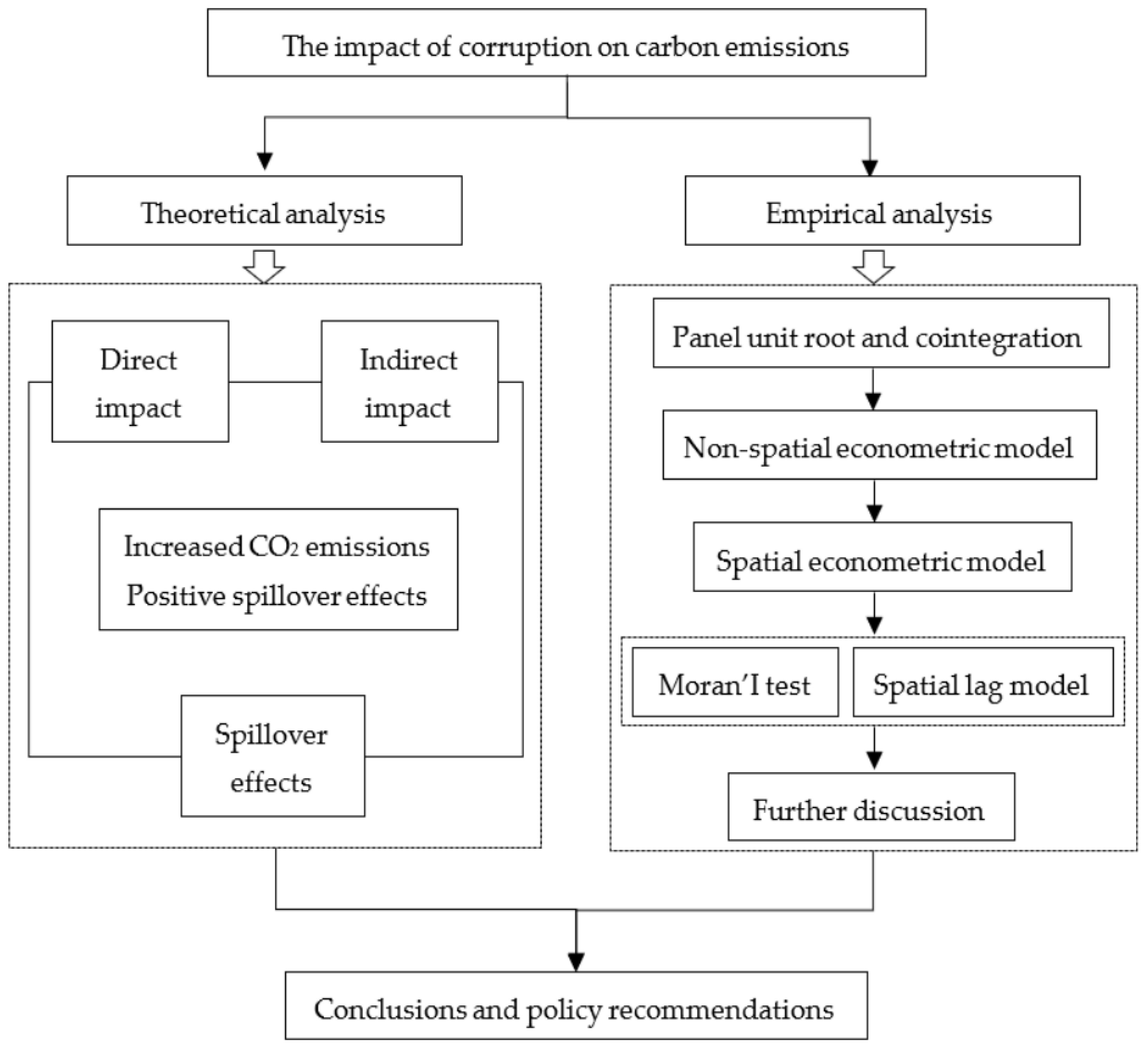
3. Theoretical Analysis and Research Hypotheses

This section aims to theoretically explore how corruption affects CO2 emissions to provide a sound theoretical basis for the subsequent empirical analysis. Specifically, this study will carry out the theoretical analysis from the following three aspects, and accordingly put forward a series of hypotheses to be tested.

3.1. The Direct Impact of Corruption on CO2 Emissions

Compared with mature market economy countries, governments in developing countries play a more important role in environmental governance. In order to realize the coordinated development of economy and environment, governments will formulate a series of strict environmental policies to regulate the production activities of enterprises. However, this will lead to polluting enterprises actively seeking rent in order to obtain a “pass” for pollution emissions, thus increasing rather than reducing CO2 emissions [48]. Theoretically, corruption can directly aggravate CO2 emissions through the “rent-seeking” effect, which is mainly reflected in three aspects, including environmental legislation, administrative enforcement and punishment, and environmental system supervision. On the one hand, corruption at the legislative level will provide legal protection for polluting enterprises at the source, which tacitly allows enterprises to discharge pollutants at will in an extensive production mode, thus leading to accelerated CO2 emissions [49]. Specifically, in order to avoid environmental supervision and maximize profits, polluting enterprises often choose to bribe policymakers to obtain political asylum. At the same time, considering that polluting enterprises are often the main contributors to the local economy, the government officials are willing to act as the “umbrella” for them to formulate loose environmental laws for their personal interests and performance appraisal, which provides legislative convenience for polluting enterprises to emit CO2. On the other hand, the strict administrative law enforcement is an important guarantee for the implementation of environmental protection policies, but negligence in law enforcement will further aggravate CO2 emissions [32]. Specifically, in order to mitigate or avoid punishment, polluting enterprises often choose to bribe environmental protection law enforcement personnel, which ultimately leads environmental law enforcement to be a mere formality. In this way, these enterprises will continue to discharge pollutants illegally, resulting in a large amount of CO2 emissions and other pollutants. In addition, due to the wide scope of environmental governance, it is very difficult for the governments to gain remarkable achievements in the short run. Therefore, effective third-party supervision cannot be implemented and can only be completed through the internal supervision mechanism, which will create favorable conditions for environmental corruption [50]. Due to the imperfect accountability mechanism, the lack of a sound supervision system, and the collusion between officials, the environmental supervision has little effect, and the efficiency of pollution control is also low, which results in the continuous increase of CO2 emissions eventually. Accordingly, the following hypothesis is proposed:
Hypothesis 1 (H1).
Corruption can directly exacerbate CO2 emissions.

3.2. The Spatial Spillover Effects of Corruption on CO2 Emissions

According to current academic studies conducted both in China and abroad, the level of carbon emissions in a country or region exhibits a substantial spatial correlation feature, which implies that the level of CO2 emissions in this given region will be affected by the neighboring countries or regions [42]. Meanwhile, in a highly centralized political and decentralized economic system, local corruption has become an important factor influencing regional environmental quality. In order to attract more investment, meet GDP performance appraisal targets, and achieve political promotion, high corruption regions tend to lower environmental standards through collusion with enterprises, eventually leading to increased CO2 emissions and environmental degradation [51]. On the other hand, the bad reputation created by corruption in some regions will also have spatial spillover effects, which will encourage other regions to compete to imitate them in order to avoid falling behind; this makes the investment in environmental governance lower than the optimal level, and ultimately results in the deterioration of overall environmental performance [52]. Moreover, if the low corruption regions strengthen environmental governance to reduce CO2 emissions, it is easy to breed “free-rider” behavior in neighboring regions, thereby dampening the enthusiasm of the low corruption regions to strengthen carbon emission governance. In this way, highly corrupt regions not only aggravate local carbon emissions, but also can bring about the “inferior competition” of prisoner’s dilemma (namely, sacrificing the environment to promote economic development) through the negative demonstration effect, thus resulting in positive spatial spillovers to CO2 emissions in neighboring regions. In addition, as a result of the political practice with Chinese features and the existence of officials’ exchange and appointment in other regions, local officials in many locations have developed into crucial disseminators of environmental governance policies. When officials from highly corrupt regions are transferred to other regions, they will also continue to emphasize economy over environmental protection, resulting in pollution spillover effects and affecting environmental governance in neighboring regions. At the same time, due to the instability of official tenure, local officials who exchange positions in different regions tend to develop the local economy at the expense of the environment in order to pursue short-term interests and position promotion, resulting in a sharp deterioration of the environmental performance of their regions. This will further exacerbate the spatial spillover effect of corruption on carbon emissions. Consequently, the following hypothesis is proposed:
Hypothesis 2 (H2).
Corruption not only aggravates local carbon emissions, but also has a significant positive impact on CO2 emissions in neighboring regions.

3.3. The Indirect Impact of Corruption on CO2 Emissions

While the inflow of foreign capital promotes the host country’s economic growth to some extent, there is also a significant worry about the carbon emissions caused by foreign enterprises [53]. In order to promote economic development, local governments compete to lower the environmental entry barrier for FDI through the “racing to the bottom” competition and gain more FDI inflows at the expense of the environment, which will indirectly affect carbon dioxide emissions. Although the entry of foreign enterprises can bring technology and capital to the host country, the environmental Kuznets curve shows that the positive impact brought about by the production scale of foreign enterprises is limited [54]. In addition, due to the persistent expansion of production scale, foreign enterprises are also facing huge demand pressure on resources in the host country. In order to eliminate the constraints of environmental policies and reduce production costs, foreign enterprises will actively seek illegal ways to obtain licenses for large-scale exploitation and inefficient production of natural resources, thereby resulting in increased energy consumption and carbon emissions. As a result, the local competition effect will weaken the effectiveness of environmental regulation, thus lowering the environmental entry barriers for FDI, which is not conducive to carbon emission governance in the region.
On the other hand, local governments have the authority to supervise and intervene in enterprises within their management scope, as well as to guide the growth of enterprises through the formulation of policies, regulations, and resource allocation [55]. This determines whether enterprises will adjust their current development model under the market competition mechanism to conform to the pertinent governmental policies. However, due to local corruption, most enterprises will decide to choose to raise non-productive expenditure while reducing R&D investment in clean technology in order to obtain political protection and enhance revenue [56,57]. These are the detrimental factors that limit the development of corporate technology and increase carbon emission. Therefore, when the governments fail to strictly enforce environmental supervision policies, enterprises’ costs associated with pollution control will be greatly reduced, and they will be less motivated to innovate, which is in opposition to the principle of maximizing social welfare. In general, the innovation distortion effect—which forces enterprises to excessively pursue the goals of profit growth and productivity improvement—causes a large number of R&D resources to be diverted to the fields of production technology improvement and capacity growth. Due to the issue of inadequate investment in energy-saving or clean emission reduction technology, this will eventually result in a low carbon emission reduction efficiency for enterprises. Based on the above analysis, we can put forward the following two research hypotheses:
Hypothesis 3 (H3).
Corruption not only directly promotes carbon emissions, but also indirectly affects CO2 emissions through the “local competition” effect.
Hypothesis 4 (H4).
Corruption not only directly aggravates carbon emissions, but also indirectly affects CO2 emissions through the “innovation distortion” effect.

4. Methods, Variables and Data Sources

4.1. Model Specification

4.1.1. Traditional Econometric Model

In earlier research on CO2 emissions, some academics adopting traditional econometric methods worked on the supposition that the spatial distribution of carbon emissions in different regions is not correlated [58]. The simple pooled linear regression model can be written without considering the introduction of spatial interaction effects:
ln C I i t = α 0 + α 1 C o r r it + α 2 ln G D P i t + α 3 I S i t + α 4 ln F D I i t + α 5 ln R D i t + μ i + γ t + ε i t
where subscripts i and t denote a specific province i (i = 1, 2, …, 30), and a given period t (t = 2003, 2004, …, 2017); lnCIit, Corrit, lnGDPit, ISit, lnFDIit, lnRDit represent carbon emission intensity, local corruption, economic development, industrial structure, foreign direct investment, and R&D investment, respectively. αi is the coefficient vector; μi represents the individual fixed effect in province i; γt represents the time-fixed effect, and εit is the stochastic error term.

4.1.2. Spatial Econometric Model

However, the above assumption does not correspond to reality. Getis [59] asserted that when spatial associations exist among states and regions, the spatial effect should not be ignored in order to avoid bias in empirical results. Hence, this study applies the spatial lag model (SLM), which improves the accuracy of the research results by combining spatial factors with traditional econometric methods. Its general form is expressed as follows:
ln C I i t = ρ j = 1 n W i j ln C I i t + X i t β + μ i + γ t + ε i t
where ρ is the spatial autoregressive coefficient; n is the number of provinces; Wij is the i, j-th element of the spatial matrix; Xit represents the vector of the independent variables at i and t, and β represents the coefficient vector.
One of the essential steps in capturing spillover effects is specifying suitable spatial weight matrices. Referring to Wu et al. [60], the geographical matrix and economic distance matrix are constructed. The geographical distance matrix (W1)—the baseline matrix in this study—is expressed as the reciprocal of the geographical distance between provinces. The straight-line distance is the actual space condition calculated according to the latitude and longitude of the provincial railway station, and the economic distance weight matrix (W2) considers the spatial effect of regional economic development. Both matrices are normalized to obtain a unified row sum.
Numerous previous studies have dwelled on using point estimation for spatial econometric analysis. Notwithstanding this, the regression coefficient for each variable cannot explain the actual marginal contribution of carbon emissions. Thus, effect decomposition is employed for further analysis. The partial derivative matrix is evaluated as follows:
ln C I X 1 k ln C I X N k = ln C I 1 X 1 k ln C I 1 X N k ln C I N X 1 k ln C I N X N k = ( I n ρ W ) 1 β k ,   ( k = 1 n )
where k is the independent variable number; In refers to the order identity matrix. The direct effect of the k-th corresponding variable, also known as the “local effect”, is recognized as the average value of diagonal elements in this coefficient matrix according to LeSage and Pace [61]. The indirect effect (i.e., the spatial spillover effect), is defined as the sum of the rows or columns of the non-diagonal elements in the determinant, and the total effect is the value of the direct effect and spatial spillover effect combined.

4.1.3. Moderating Effect Model

To further investigate the mechanism effect of corruption on CO2 emissions, the interaction term between corruption and foreign direct investment (Corr × lnFDI) and between corruption and R&D investment (Corr × lnRD) are added to Equation (2), respectively. The following model can be obtained:
ln C I i t = ρ j = 1 n W i j ln C I i t + X i t β + δ i ( C o r r i t × Z i t ) + μ i + γ t + ε i t
where Zit represents the foreign direct investment or R&D investment; δi represents the coefficient of the interaction term and the other symbols represent the same as in Equation (2).

4.2. Variables and Data Sources

4.2.1. Dependent Variable

Carbon emission intensity (lnCI). On the premise of consulting the energy statistics report and complying with the international criterion of energy balance, the calculation of total CO2 emissions is made on seven typical fossil fuels, including kerosene, gasoline, coke, diesel, fuel oil, coal, and natural gas. Carbon emissions generated from cement production were also taken into consideration. Following Du et al. [62], the specific calculation formula for total carbon emissions is expressed as follows:
C E = i = 1 7 Q i × C F i × C C i × C O F i × 44 12 + Q × E F c e m e n t
where CE is the total amount of carbon emission generated from various energy sources and cement production, and Qi represents the corresponding energy consumption. CFi denotes the calorific factor of fuel, CCi refers to the carbon content, COFi denotes the carbon oxidization factor, Q is the cement output, and EFcement is the emission factor of cement production.
In this study, the dependent variable is expressed as carbon emission per unit of GDP, i.e., carbon emission intensity, and its logarithmic form is taken. Generally, carbon emission intensity is designed to measure the efficiency of contamination control, that is, the lower the carbon emission intensity, the greater the efficiency of carbon mitigation, and vice versa. To intuitively reflect the regional variations and the spatio–temporal evolution in pollution emissions as time progresses, Figure 2 depicts the provincial levels of carbon emissions in 2003 and 2017.

4.2.2. Independent Variable

Local corruption (Corr). How to measure the degree of corruption has always been the focus of academic discussion due to the concealment of corruption and the fact that different countries have different standards for measuring corruption. The Extractive Industries Transparency Initiative (EITI), for example, has focused on corruption in mining, arguing that the failure of resource-rich developing countries to develop, that is, that they suffer from a “resource curse”, is mainly due to government corruption [63,64]. It advocates for revealing corruption by increasing transparency in the management of natural resources. At present, there are two main methods to measure corruption, one is based on subjective measurement and the other is based on objective measurement. Subjective measurement methods mainly rely on the evaluation scores of the questionnaire (public, experts, enterprises, etc.) to obtain a series of indicators. Many subjective measurement methods are widely used around the world, such as the Corruption Perception Index (CPI) and Bribery Perception Index (BPI) published by Transparency International, etc. In addition to establishing various subjective indicator systems in the form of questionnaires, objective measurement methods to measure the level of corruption through the number of corruption or criminal cases investigated by the state judiciary are often used. For example, Goel and Rich [65] established an indicator to measure the degree of corruption in states based on the number of civil servants convicted of abuses of power in American states. Since the former is subjective in questionnaire settings and personnel evaluations, and regional-level research data are difficult to obtain, this paper employs the latter to assess the corruption level of each region. Referring to Fisman and Gatti [66], we adopted the ratio of the number of job-related crimes investigated by the provincial people’s procuratorate each year to the number of public officials in the province to reflect the degree of corruption, which is specifically expressed as the total number of corruption, bribery, malfeasance, and infringement cases filed per 10 thousand public officials in the region (Corr, pieces/10,000 persons). The original data on corruption in each province was mainly obtained by consulting the Procuratorial Yearbook of China and the relevant local legal Yearbook, Economic Yearbook and local government report. However, since the reform of China’s supervision system was implemented in 2018, the data on job-related crime in all provinces and cities are no longer published. Therefore, based on the principle of strong data availability and less interference factors, the data from 30 provinces between 2003 and 2017 are selected as typical samples in this paper. It should also be noted that during the sample period, the Procuratorial Yearbook of some provinces did not release the cases put on file in certain years. To ensure the integrity of data, the interpolation method was applied to supplement such missing data.

4.2.3. Moderating Variables

To facilitate further discussion on the impact of corruption on CO2 emissions, foreign direct investment and R&D investment were incorporated into the mechanism analysis.
Foreign direct investment (lnFDI). This study applied the actual annual proportion of foreign investment to the total population of each province. Up until now, views about the relationship between FDI and pollutant emissions have fallen into two main categories, namely, the “pollution haven” hypothesis and the “pollution halo” hypothesis [67].
R&D investment (lnRD). This variable was measured by R&D expenditure per capita. Some scholars have found that R&D investment contributes to carbon emission reduction [21]. However, this is not an absolute conclusion, which largely depends on the efficiency of technological innovation [23].

4.2.4. Control Variables

To address the issue of missing variables, our research also selected two additional representative variables, economic growth (lnGDP) and industrial structure (IS), as the control variables for the next analysis. The real GDP per capita in this paper is employed as an indicator of the level of economic progress. According to the EKC theory, when the economy turns to high-quality growth, pollution will decrease with the improvement of economic growth levels [18]; therefore, the measure of industrial structure is expressed as the proportion of regional tertiary industry output value to the second industrial increment in value in this paper. Zheng et al. [68] claimed that the more advanced the industrial structure, the more conducive to low-carbon development.

4.2.5. Data Sources

The descriptive analysis of each variable is presented in Table 2. Panel data covering 30 provinces of China (excluding Tibet, Hong Kong, Macao, and Taiwan) spanning 2003 to 2017 are selected for analysis. For the incomplete data of some variables, interpolation was utilized to fill in the relevant missing data. The original data were mainly collected from the National Bureau of Statistics, China Statistical Yearbook of Environment and China Energy Statistical Yearbook. To eliminate the inflation effect, this study deflated the applicable nominal data based on the 2003 constant price. Some data were logarithmically processed to reduce the heteroscedasticity. We then tested whether multicollinearity exists among the selected variables. According to the test results, the variance inflation factors of the explanatory variables are less than 10, indicating that there is no obvious multicollinearity problem. Thus, the selection of all variables was reasonable.

5. Results and Discussion

5.1. Panel Unit Root and Cointegration Test

Panel unit root tests are required as preliminary work before regression analysis to avoid the problem of “spurious regression”. The research on the comparison of unit root tests of LLC, IPS, ADF-Fisher, and PP-Fisher is carried out in this paper. All four tests assume the existence of a unit root process. As shown in Table 3, the first differences of relevant variables do not fail to test significance, which implies that all variables are integrated of order one, so the panel co-integration test can be performed. The panel cointegration approach comprising the Pedroni test and Kao test is employed, and the results are illustrated in Table 4. Specifically, the Pedroni test results show that regardless of the AR coefficient based on the within-dimension or between-dimension dimensions, both PP-statistics and ADF-statistics reject the null hypothesis, i.e., there is no co-integration relationship at a 1% critical value. Additionally, the Kao-ADF statistic of the panel data is significant at the 10% confidence level, confirming the paper’s findings about the stable co-integration relationship between CO2 emissions and the independent variables chosen. So, as discovered by the above research, variables Corr, lnGDP, lnFDI, IS, and lnRD are co-integrated with lnCI, thus admitting the presence of long-term equilibrium correlation.

5.2. Non-Spatial Econometric Analysis

In order to better highlight the superiority of the spatial econometric model, this study applied a series of traditional econometric analysis methods to conduct comparative regression verification. Firstly, the pooled ordinary least squares method (POLS) is used to estimate Equation (1), and the coefficient of corruption is significantly positive, which is consistent with Dincer and Fredriksson [36]. Their analysis shows that corruption leads environmental supervision departments to loosen environmental regulations, reduce law enforcement, and allow polluting enterprises to pay a modest amount of benefits in exchange for a “pass” on pollution emissions. In this way, resource allocation is thus distorted as a result of corruption and bribery, which ruins the environment and increases CO2 emissions. Then, this paper introduces fixed effects (FE) and random effects (RE) to solve the possible individual and time heterogeneity, and conducts the Hausman test on the estimation results. The statistical value of the Hausman test abandons the null hypothesis, so fixed effects are chosen. In addition, the panel data were re-estimated using the generalized least squares method (FGLS) for controlling potential first-order autoregression and heteroscedasticity. The empirical results in Table 5 suggest that the estimated coefficient of corruption on CO2 emissions is significantly positive at the level of 5%—that is, corruption will cause the emitting of CO2 emissions. Finally, considering the possible endogenous problems between variables [69], the system generalized method of moments (SYS-GMM) is applied to address this issue, and we also adopted the difference generalized method of moments (DIFF-GMM) to enhance the reliability of empirical results. Both the AR test and Hansen overidentification test demonstrate that the results of SYS-GMM and DIFF-GMM are credible. In summary, no matter what estimation method is adopted, the environment will deteriorate as corruption levels rise. Therefore, Hypothesis 1 (H1) is verified.

5.3. Spatial Econometric Analysis

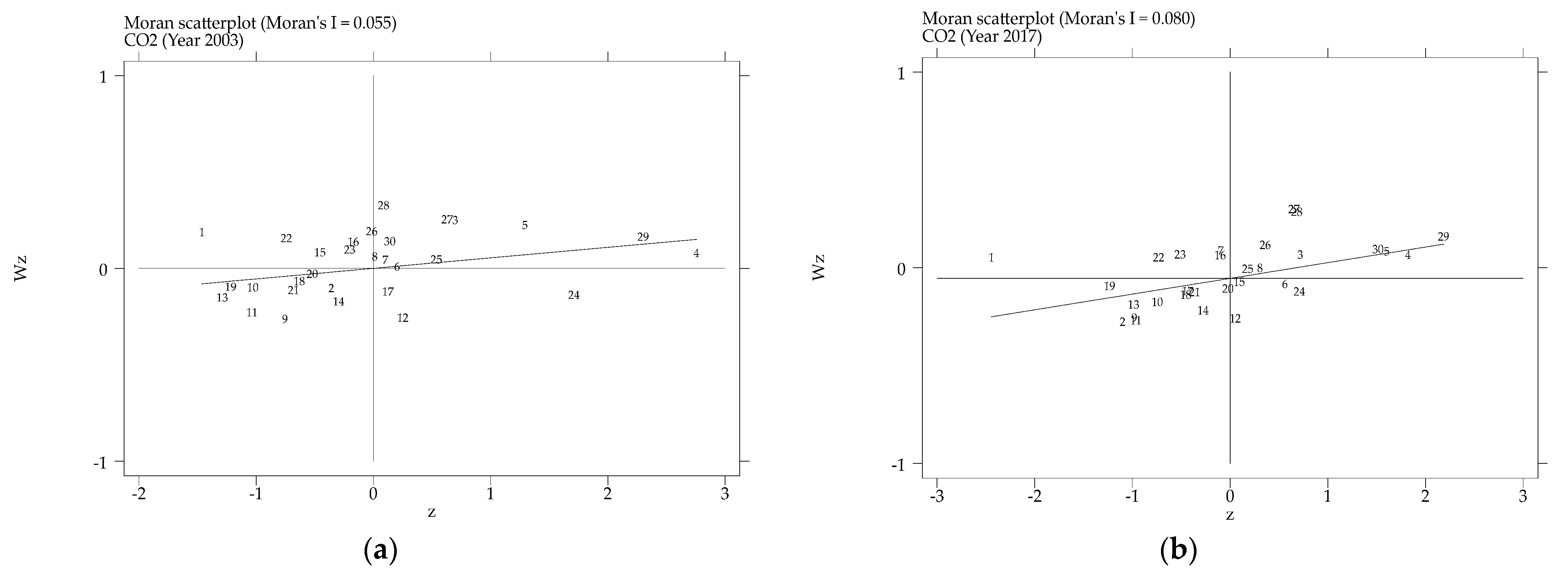
5.3.1. Spatial Autocorrelation Analysis

There are numerous methods for spatial correlation testing, mainly including Moran’s I, Geary’s C, and Getis-Ord. Following the mainstream methods in the existing literature [70], we introduce the global Moran’s I to examine the spatial correlation of carbon emissions. The corresponding formula is illustrated in Equation (6):
Global   Moran s   I = n i = 1 n j = 1 n W ij ( Y i Y ¯ ) ( Y j Y ¯ ) i = 1 n j = 1 n W i j i = 1 n ( Y i Y ¯ ) 2
where Y ¯ = 1 n i = 1 n Y i ,Yi and Yj are the carbon intensity of provinces i and j respectively; n represents the number of regions; and Wij denotes the element of the spatial matrix.
The range of the global Moran’s I statistic is [−1, 1]. The degree of spatial correlation and the absolute value of global Moran’s I are in direct proportion when specifying the significance level, and it indicates that there is no spatial association if this value equals zero. The values of Moran’s I during the period 2003–2017 are shown in Table 6. All values within 15 years under the geographical distance weight matrix (W1) and economic geographical distance matrix (W3) are positive at a 1% critical value. Except for 2003–2006, all other years’ values of global Moran’s I under the economic matrix (W2) are positive and pass the 10% significance test. The results demonstrate that the distribution of provincial carbon emission intensity is not random, but instead reflects spatial agglomeration. Consequently, if the spatial effect is not taken into account when discussing the influence of corruption on CO2 emissions, it is hard to draw conclusions that conform to the actual situation. The global Moran’s I can illustrate the overall spatial association, while the local Moran’s I can measure the regional spatial correlation well. Hence, the method of local Moran’s I is applied to reveal the specific spatial structure of carbon emissions on a more detailed scale, so as to illustrate the local spatial cluster. The formula can be expressed as follows:
Local   Moran s   I = n ( Y i Y ¯ ) i = 1 n ( Y i Y ¯ ) 2 j = 1 , j i n W i j ( Y j Y ¯ )
The spatial dependence of provincial carbon intensity in China shown in Table 6 is gradually increasing. We then depicted Moran scatter plots for 2003 and 2017 based on the geographic distance matrix (W1) for comparison. In Figure 3, the horizontal axis represents the normalized carbon intensity, while the vertical axis indicates the spatial lag value. Additionally, the first and third quadrants indicate that carbon intensity is spatially high-high or low-low concentrated, whereas the second and fourth quadrants indicate that there is no consistency in the carbon intensity of regions with close spatial proximity. As shown in Figure 3, the majority of provinces belong to the I (high–high) and III (low–low) quadrants. Thus, it can be determined that carbon emission intensity exhibits significant spatial agglomeration characteristics. To acquire more precise empirical results, spatial econometric approaches must be implemented in accordance with the aforementioned spatial correlation analysis.

5.3.2. Results of Spatial Econometric Model

Determining a suitable spatial econometric model is needed before proceeding with empirical analysis. According to the Hausman test above, it is confirmed that the fixed effect model is superior to the random effect model. Then, following Elhorst [71], we conduct four fixed effects analyses. After the Lagrange multiplier (LM) test, displayed in Table 7, the SLM with two-way fixed effects is selected for all specifications. To demonstrate the effect of corruption on CO2 emissions, especially to verify the spatial spillover effect between them, we conduct spatial benchmark regression next, as described in Table 8. Moreover, the estimated results of the SEM and the SDM are reported as references. For the empirical parts, it is found that the spatial autoregressive coefficient (ρ) indicates a persistently positive value, implying that there is distinct heterogeneity in the spatial distribution of China’s carbon emissions, which also shows the feasibility of the spatial econometric model.
The estimation under various matrices indicates that at a level of 1%, when holding other factors constant, the estimation coefficient of the core explanatory variable corruption is significantly positive, showing that corruption will promote carbon dioxide production. This result is similar to the research conclusions drawn by Ren et al. [37]. China’s local environmental protection departments lack independence as a result of the powers cross in exercising. Institutional factors may compromise the efficiency of enforcing environmental regulations to a certain extent by reducing the stringency of environmental law and its enforcement [72]. Regarding the control variables, the results of W1 and W2 also underline that the improvement of the economic level, the increase in FDI, and the upgrading of the industrial structure are beneficial for carbon emission reduction. The coefficient of GDP is significantly negative, indicating that economic growth can effectively reduce CO2 emissions, which also verifies the existence of economies of scale. This also implies that China can still meet the demands of carbon emission reduction despite its economic prosperity and progress under the new normal. The specific effect of foreign investment on CO2 emissions has been controversial, but the empirical results of this paper show that the “pollution haven” effect of FDI has not yet appeared in China. The regression result for industrial structure is in line with expectations, which confirms that the upgrading of industrial structure and the green transformation of the industry can effectively reduce CO2 emissions. However, inconsistent with our prediction, the investment in technological research can worsen the process of carbon emission reduction, which is consistent with the findings obtained by Amri et al. [23]. The main reason may be that although China has invested heavily in scientific research, the problem of the low conversion rate of scientific and technological achievements has not been effectively solved and current resource allocations are not asymmetrical, eventually leading to the phenomenon of poor efficiency in emission reduction.
Owing to the existence of spatial spillovers, the coefficient of corruption cannot be interpreted as the impact on CO2 emissions alone. As such, to better illustrate the specific effects of corruption, a vector partial differential method is required to decompose the overall spatial effect according to the regression results above. As indicated, the results of the geographic weight matrix, displayed in Table 9, manifest that both the indirect and overall effects of corruption are significantly positive at the 5% critical value, while the direct effect is positive and reaches the significance level of 1%. This conclusion is also consistent with the findings of Yin et al. [52]. These findings suggest that, in general, corruption shows a curbing impact on carbon reduction and, in particular, corruption has positive spatial spillovers on CO2 emissions, indicating that a neighboring province with high levels of corruption will boost carbon dioxide production within the area. Driven by the promotion mechanism, provinces with high levels of corruption will obtain economic and political dividends by relaxing environmental controls on polluting enterprises. However, due to the existence of “inferior competition”, these provinces will provide a bad template for their neighboring provinces, which will worsen the environmental performance of neighboring regions and increase CO2 emissions. In addition, the negative externalities of the environment also provide local governments with free-riding opportunities, which will further reduce carbon emission reduction efficiency. Thus, Hypothesis 2 (H2) is verified. In contrast, in the application of the economic weight matrix, the overall effect coefficient of corruption is 0.0356, and it satisfies the statistical test, which implies that corruption can exacerbate China’s carbon pollution. Additionally, both the direct and indirect effects of corruption are significantly positive, and the direct effect exhibits more inhibition on carbon emission reduction than the indirect effect, indicating that the degree of local carbon emissions is influenced by spatially related regions, but primarily by the level of corruption in the region. Moreover, the spatial spillovers of all control variables are significant. Specifically, the level of economic growth, FDI, and industrial structure all have adverse direct effects and spatial spillovers, implying that the improvement of these factors in this region is conducive to promoting carbon emission reduction in neighboring regions, while R&D investment in this region will exacerbate the pollutant discharge in adjacent regions. This may be because, in the process of production and research, high-polluting and energy-consuming plants are relocated to nearby areas, thus exacerbating CO2 emissions.

5.3.3. Regional Heterogeneity Analysis

China is noted for its vast territories and there are striking regional differences in the economy, the environment, and so on. In the ensuing discussion, the paper further explores whether spatial heterogeneity is established at the regional level. According to the regional division method of the National Bureau of Statistics, three sub-samples of the eastern, central, and western regions are established to re-estimate. The estimated coefficients and their effect decomposition results are reported in Table 10. According to the analysis of the eastern sub-sample, the coefficients in the eastern region are consistent with the benchmark regression results. Although the parameter values change, the symbols remain the same. Additionally, the direct and spatial impacts of corruption are 0.0395 and −0.0105, respectively, but only the direct effect is significant, indicating that the direct effect plays a primary role in the significant positive total effect of corruption on promoting pollutant discharge. Therefore, for the eastern area, the direct impact of local corruption is a crucial conduit affecting CO2 emissions. The empirical results in the central region show that, for corruption, the direct effect (−0.0192) is significantly negative, whereas the spillover effect (0.0106) is significant with a positive sign. This may be because China’s power center is located in the central region, where political competition is more intense and environmental policies are implemented more vigorously. Therefore, the direct effect of corruption in the central region is negative. Although the surrounding provinces with a high degree of corruption will increase the carbon emissions of the region, the overall effect in the central region is ultimately negative (−0.0086), as the direct effect is stronger than the indirect effect. Additionally, the direct and spillover impacts of the western region are both negative, which means that corruption improves carbon emission reduction performance, yet the significance is not remarkable in statistics. This means that corruption promotes carbon emission reduction. The possible reason is that corruption in the western region has increased the “rent-seeking cost” of enterprises engaged in production and operation activities, making polluting enterprises more advantageous than clean enterprises in terms of production costs, leading to clean enterprises being driven out of the market. Therefore, carbon emissions will temporarily decrease in the short term as the number of manufacturing enterprises decreases. However, it must be pointed out that this emission reduction effect is inefficient and is not conducive to the long-term development of the region in the future. To sum up, different factors not only have heterogeneity in their direct impact on local and regional pollutant emissions, but also have varying spillover effects on CO2 emissions from neighboring provinces, resulting in the complexity of pollution treatment in different regions.

5.3.4. Robustness Tests

For reasons of validating the reliability of the above main findings, the robustness checks given in Table 11 are constructed from three aspects: alternative indicators, sample intervals, and a spatial weight matrix. The first robustness test employs an alternative indicator of corruption, which is expressed by the logarithm of the number of annual corruption, bribery, and malfeasance cases in each province, to check whether the main conclusions changed or not and to obtain a unanimous conclusion. Furthermore, the results of control variables only differ in the coefficient values. Therefore, the results presented in this paper are robust. The second robustness test changes the research period. As mentioned above, since the procuratorial yearbooks of some provinces did not report the relevant number of cases filed in the current year, this paper made up such missing data based on the existing data. In order to avoid the processed data interfering with the testing results, we adjusted the sample to 2006–2017. The influence coefficients of corruption on CO2 emissions are still significantly positive under the geographical distance matrix, which confirms the robustness of our results as well. What is interesting is that the level of significance of the industrial structure changes. Although its regression coefficient is still negative, it becomes insignificant. This may be due to the shortening of the sample period, making its emission reduction effect less obvious. Under the economic–geographical weight matrix (W3), corruption exerts positive impacts on CO2 emissions, and the estimated coefficients and significance levels remain essentially the same in the third robustness test. The regression results of the control variables also support the previous conclusions. This indicates that the conclusions of the empirical model test are sure-footed and reliable. Last but not least, the direct impact and spatial spillovers of each explanatory variable under W1 are also analyzed. The findings of effect decomposition suggest that although the parameter values change, their significance and signs have not altered much. The conclusions drawn in Table 8 and Table 9 are also validated in Table 11. Therefore, the main discoveries of the above-mentioned benchmark testing can be considered credible.

5.4. Further Discussion

5.4.1. Moderating Effect Analysis

In order to conduct mechanism analysis, this study introduces the interaction terms of FDI and corruption as well as R&D investment and corruption, respectively, and the SLM is used to estimate Equation (4). The decomposition results of spatial effects after adding interaction terms are shown in Table 12. From the regression analysis of FDI, the direct effect of the interaction term (Corr × lnFDI) and the spatial spillover effects are significantly positive under W1. The research results almost fully support Hypothesis 3 (H3), that is, that a higher level of FDI will exert a more significant positive moderating effect on the process of corruption affecting pollutant emissions in this region and other regions. For the two reasons set out below, for one thing, the pressure of an achievement inspection such as GDP urges local authorities to launch the deteriorating competition of environmental regulation, that is, a “race to the bottom” to attract foreign investment and vigorously develop the regional economy. In this way, due to the “local competition” effect, a large number of low-quality foreign enterprises are introduced, which makes local pollution worse [53]. For another, loose environmental regulations will attract other pollution-intensive industries, which will further aggravate the local exhaust emissions of pollutants such as carbon dioxide [54]. To sum up, the interaction between FDI and corruption eventually leads to an increase in CO2 emissions.
From the estimated results after adding the interactive term (Corr × lnRD), R&D investment can also play a significant moderating role in the process of corruption affecting pollutant emissions, but it does not fulfill the expectations of adjustment and improvement. It could be partly due to the existence of the “innovation distortion” effect, enterprises’ production factors such as manpower, capital, and technology cannot realize effective allocation, resulting in a lack of innovation motivation for enterprises to carry out clean production, which leads to an increase in carbon emissions [57]. In addition, although China has invested heavily in scientific research, the problem of the low conversion rate of scientific and technological achievements has not been effectively solved due to the limited innovation ability of enterprises, which leads to the fact that the emission reduction effectiveness of clean technology has not been realized. Therefore, in this case, due to the innovation distortion and improper allocation of enterprises’ R&D investments, the technological innovation efficiency of enterprises will be reduced and, finally, the hindrance effect of corruption on carbon emission reduction efficiency will be intensified. Hence, Hypothesis 4 (H4) is verified.

5.4.2. Anti-Corruption Campaign Policy Analysis

As an important part of the construction of political civilization, the role of combating corruption becomes more prominent. The Chinese authorities made numerous efforts and achieved remarkable success in pushing hard for anti-corruption work. Especially in 2012, the Chinese government launched a nationwide crackdown, applying stricter laws, tougher enforcement, and sterner punishment than ever before, and upholding the fight between tigers and flies at the same time. During this period, the central government also continuously advanced the construction of an ecological civilization, with special emphasis on environmental protection. Considering that environmental performance is closely related to government activities, exploring whether high-pressure anti-corruption will exert a positive influence on local environmental governance deserves further study. Hence, taking the anti-corruption events in 2012 as the starting point, we divided the sample period into two parts, 2003–2012 and 2013–2017, to evaluate the effect of anti-corruption on the two sub-samples. The estimation results obtained by segmented regression based on Equation (2) can be seen in Table 13.
The findings of the first group (2003–2012), represented in Table 13, show that before the implementation of the strict anti-corruption campaign, corruption had a promoting effect on the CO2 emissions of the local and neighboring areas, but mainly on local carbon emissions. In order to obtain greater benefits with low costs and high emissions, polluting enterprises tend to cooperate by delivering benefits to officials in exchange for avoiding environmental regulation. Thus, corruption undermines the effectiveness of environmental policies and leads to increased pollution. In the second group (2013–2017), the estimated coefficient of the direct and indirect impact of corruption is negative but not significant, indicating that corruption reduces CO2 emissions. Cracking down on corruption may act as an effective deterrent for government officials so that local governments dare not corrupt and take the initiative to participate in environmental governance to cope with performance appraisal. Thus, we can see that the sign of the corruption coefficient in the segmented regression results has changed significantly, which also verifies that anti-corruption is conducive to the reduction of carbon emissions to a certain extent. However, this could be due to the study’s small sample size, which makes the regression results of the two groups insignificant and, as a result, fails to fully reveal the reduction effect of anti-corruption efforts on CO2 emissions.

6. Conclusions and Policy Implications

Facing the sharp contradiction between environment carrying capacity and sustainable development strategy, energy conservation and emission reduction has become a global consensus. There is no exception for China as well. Meanwhile, corruption, as an institutional factor affecting economic development, also plays a major role in environmental quality. In this context, this paper collects China’s provincial panel data, spanning the period 2003–2017, and empirically tests the impact of corruption on CO2 emissions by using the spatial econometric model. In particular, it focuses on whether there are spatial spillovers of corruption on CO2 emissions. The main conclusions of this paper are drawn as follows: Firstly, the empirical findings of this study show that there is distinct heterogeneity in the spatial distribution of China’s CO2 emissions. Secondly, it verifies that corruption will worsen regional CO2 emissions. More importantly, based on the spatial effect decomposition, it has also found that corruption will not only aggravate CO2 emissions in the region, but also stimulate carbon emissions in neighboring regions. Thirdly, the spatial effect of corruption on CO2 emissions shows significant regional heterogeneity. Specifically, local corruption in the eastern region has significantly increased CO2 emissions, while corruption in the central and western regions is negatively related to carbon emissions, but the coefficients are not significant. Fourth, the interaction term between FDI and corruption, as well as the interaction term between R&D investment and corruption, significantly promotes CO2 emissions. Moreover, the spatial spillover effects of the two are also significantly positive, indicating that technological innovation and FDI not only fail to mitigate carbon emission reduction in this region, but also further promote CO2 emissions in neighboring regions, which is known as the convergence effect. This shows that corruption has resulted in the distortion of local government competition and innovation resources.
To resolutely win the battle against corruption and achieve the solemn goals set by the 20th National Congress, the Chinese government should take vigorous measures to promote anti-corruption and energy conservation. Based on the above research, we put forward the following policy recommendations:
First, the government should accelerate low-carbon transformation and guide the construction of a fair, reasonable, and win-win environmental protection system. Specifically, on the one hand, the state and local governments should promote green and sustainable economic and social development by improving environmental governance, strengthening regional ecological compensation, and constructing main ecological functional areas. On the other hand, due to regional heterogeneity in CO2 emissions, governments should enhance the awareness of coordinated management, strengthen the exchanges and cooperation at the provincial level, and intensify the overall effect of energy conservation and emission reduction. In addition, raising national awareness of environmental protection and advocating for the formation of a green and low-carbon lifestyle can effectively promote green development.
Second, China’s regulatory authorities should vigorously promote the construction of a system for punishing and preventing corruption. As proposed at the 20th National Congress, as long as there exists the soil and conditions for corruption, the fight against corruption will not stop for a moment. Therefore, we must always continue to deepen the legal system against corruption, adhere to the comprehensive promotion of anti-corruption and integrity, and adopt a zero-tolerance attitude towards corruption. China’s scientific anti-corruption strategy and resolute have also set an example for the world and provided referential experiences. Concretely, while maintaining the independence of law enforcement power, authorities should make good use of the vertical management of local environmental supervision and law enforcement departments to ensure the orderly operation of environmental laws and regulations. Meanwhile, local governments should systematically combine anti-corruption with regional environmental governance and stress control over the frequent occurrence of corruption in the field of environmental protection. Moreover, a series of supporting anti-corruption measures, such as improving the monitoring system, standardizing the assessment mechanism, and public advocacy should be developed.
Third, local governments should pay more attention to the quality of FDI and optimize the domestic investment environment, so as to attract higher-quality foreign investment and give play to their role as a “pollution halo” in China. The technology spillover effect can promote the technological innovation of local enterprises and can also form a forced mechanism for domestic polluting enterprises to promote transformation and upgrading, thereby reducing CO2 emissions. This is of great significance to realizing the goal of “improving the comprehensive quality of foreign capital utilization”. In addition, the development of a low carbon and circular economy requires green technological innovation as a pillar. In the 14th Five-Year Plan, China clearly stated that it would accelerate the development strategy of building strategic scientific and technological forces. This requires the governments to constantly optimize the allocation of innovation resources while adhering to the two-wheel driven development of scientific and technological innovation and institutional innovation. Thus, efforts should be made to improve the level of clean energy technology and energy utilization efficiency, and effectively solve problems such as the transformation and application of technological achievements, from theoretical research to production practice.
Last but not least, China should strive to promote anti-corruption and environmental protection while maintaining sustained and stable economic development under the “new normal”. Specifically, the Chinese authorities should establish and improve relevant systems, and give full play to the coordination of carbon emission reduction, economic growth and corruption governance. At the same time, the governments should properly settle the conflict between industrial structure transformation and energy consumption, optimize the energy consumption structure, and gradually replace traditional fossil energy with clean energy, such as wind energy and solar energy. In addition, governments should also focus on promoting supply-side structural reform, force the closure of industries with high energy consumption and high pollution, and promote the comprehensive transformation and upgrading of industrial industries to achieve carbon emission reduction.

7. Limitations and Outlook

Although this study quantitatively explored the spatial spillover effect of local corruption on China’s regional carbon emissions, there are still a lot of limitations that require further exploration. Firstly, the paper conducts empirical analysis by employing the static model, and the possible time lag is not taken into account. Therefore, dynamic spatial econometric models, such as the dynamic spatial GMM model, should be introduced in future to explore the linkage between corruption and CO2 emissions from spatio-temporal dimensions and to overcome the possible endogeneity problem. Second, limited by difficulties in obtaining corruption data, this paper just investigates the impact of corruption on CO2 emissions based on the provincial panel data, which may affect the rationality of conclusions. Therefore, in order to make our empirical results more reliable, if we expand the research sample to prefecture-level cities in the future, it is of great significance to strengthen the corruption governance for grass-roots governments. Finally, because of the short evaluation period and limited sample size, the empirical method used in this paper cannot accurately reflect the evolution of various anti-corruption policies. Given this, in order to provide a useful reference, we will attempt to use the staggered DID model to analyze policy shocks in the future.

Author Contributions

Conceptualization, X.X.; methodology, X.X.; investigation, B.Y.; data curation, B.Y.; writing—original draft preparation, B.Y.; writing—review and editing, X.X.; supervision, X.X.; funding acquisition, X.X. All authors have read and agreed to the published version of the manuscript.

Funding

This research was funded by the National Social Science Foundation of China (No. 19BRK036), the Humanities and Social Science Youth Foundation of the Ministry of Education in China (No. 18YJC840047), and the Social Science Foundation of Hunan Province (No. 17YBQ104).

Institutional Review Board Statement

Not applicable.

Informed Consent Statement

Not applicable.

Data Availability Statement

Not applicable.

Conflicts of Interest

The authors declare no conflict of interest.

References

  1. Weitzel, M.; Ma, T. Emissions embodied in Chinese exports taking into account the special export structure of China. Energy Econ. 2014, 45, 45–52. [Google Scholar] [CrossRef] [Green Version]
  2. Wang, G.; Deng, X.; Wang, J.; Zhang, F.; Liang, S. Carbon emission efficiency in China: A spatial panel data analysis. China Econ. Rev. 2019, 56, 101313. [Google Scholar] [CrossRef]
  3. Barrows, G.; Ollivier, H. Foreign demand, developing country exports, and CO2 emissions: Firm-level evidence from India. J. Dev. Econ. 2021, 149, 102587. [Google Scholar] [CrossRef]
  4. Xu, B.; Lin, B. How industrialization and urbanization process impacts on CO2 emissions in China: Evidence from nonparametric additive regression models. Energy Econ. 2015, 48, 188–202. [Google Scholar] [CrossRef]
  5. Xu, X.; Li, S. Neighbor-Companion or Neighbor-Beggar? Estimating the Spatial Spillover Effects of Fiscal Decentralization on China’s Carbon Emissions Based on Spatial Econometric Analysis. Sustainability 2022, 14, 9884. [Google Scholar] [CrossRef]
  6. Cui, L.; Li, R.; Song, M.; Zhu, L. Can China achieve its 2030 energy development targets by fulfilling carbon intensity reduction commitments? Energy Econ. 2019, 83, 61–73. [Google Scholar] [CrossRef]
  7. Dong, F.; Hua, Y.; Yu, B. Peak Carbon Emissions in China: Status, Key Factors and Countermeasures—A Literature Review. Sustainability 2018, 10, 2895. [Google Scholar] [CrossRef] [Green Version]
  8. Gong, W.; Wang, C.; Fan, Z.; Xu, Y. Drivers of the peaking and decoupling between CO2 emissions and economic growth around 2030 in China. Environ. Sci. Pollut. Res. 2022, 29, 3864–3878. [Google Scholar] [CrossRef]
  9. Esfahani, H.S.; Ramırez, M.T. Institutions, infrastructure, and economic growth. J. Dev. Econ. 2003, 70, 443–477. [Google Scholar] [CrossRef]
  10. Lee, C.C.; Chang, C.H.; Arouri, M.; Lee, C.C. Economic growth and insurance development: The role of institutional environments. Econ. Model. 2016, 59, 361–369. [Google Scholar] [CrossRef]
  11. Qiang, Q.; Jian, C. Natural resource endowment, institutional quality and China’s regional economic growth. Resour. Policy 2020, 66, 101644. [Google Scholar] [CrossRef]
  12. Seldadyo, H.; De Haan, J. Is corruption really persistent? Pac. Econ. Rev. 2011, 16, 192–206. [Google Scholar] [CrossRef]
  13. Deng, J. The National Supervision Commission: A new anti-corruption model in China. Int. J. Law Crime Justice 2018, 52, 58–73. [Google Scholar] [CrossRef]
  14. Lin, S.; Zhao, D.; Marinova, D. Analysis of the environmental impact of China based on STIRPAT model. Environ. Impact Assess. Rev. 2009, 29, 341–347. [Google Scholar] [CrossRef]
  15. Wang, Y.; Kang, Y.; Wang, J.; Xu, L. Panel estimation for the impacts of population-related factors on CO2 emissions: A regional analysis in China. Ecol. Indic. 2017, 78, 322–330. [Google Scholar] [CrossRef]
  16. Halicioglu, F. An econometric study of CO2 emissions, energy consumption, income and foreign trade in Turkey. Energy Policy 2009, 37, 1156–1164. [Google Scholar] [CrossRef] [Green Version]
  17. Alam, M.M.; Murad, M.W.; Noman, A.H.M.; Ozturk, I. Relationships among carbon emissions, economic growth, energy consumption and population growth: Testing Environmental Kuznets Curve hypothesis for Brazil, China, India and Indonesia. Ecol. Indic. 2016, 70, 466–479. [Google Scholar] [CrossRef]
  18. Shahbaz, M.; Haouas, I.; Van Hoang, T.H. Economic growth and environmental degradation in Vietnam: Is the environmental Kuznets curve a complete picture? Emerg. Mark. Rev. 2019, 38, 197–218. [Google Scholar] [CrossRef]
  19. Wang, G.; Chen, X.; Zhang, Z.; Niu, C. Influencing Factors of Energy-Related CO2 Emissions in China: A Decomposition Analysis. Sustainability 2015, 7, 14408–14426. [Google Scholar] [CrossRef] [Green Version]
  20. Wu, L.; Sun, L.; Qi, P.; Ren, X.; Sun, X. Energy endowment, industrial structure upgrading, and CO2 emissions in China: Revisiting resource curse in the context of carbon emissions. Resour. Policy 2021, 74, 102329. [Google Scholar] [CrossRef]
  21. Wang, Z.; Yin, F.; Zhang, Y.; Zhang, X. An empirical research on the influencing factors of regional CO2 emissions: Evidence from Beijing city, China. Appl. Energy 2012, 100, 277–284. [Google Scholar] [CrossRef]
  22. Chen, J.; Gao, M.; Ma, K.; Song, M. Different effects of technological progress on China’s carbon emissions based on sustainable development. Bus. Strateg. Environ. 2020, 29, 481–492. [Google Scholar] [CrossRef]
  23. Amri, F.; Zaied, Y.B.; Lahouel, B.B. ICT, total factor productivity, and carbon dioxide emissions in Tunisia. Technol. Forecast. Soc. Chang. 2019, 146, 212–217. [Google Scholar] [CrossRef]
  24. Liang, Q.M.; Fan, Y.; Wei, Y.M. Carbon taxation policy in China: How to protect energy- and trade-intensive sectors? J. Policy Model. 2007, 29, 311–333. [Google Scholar] [CrossRef]
  25. Mardones, C.; Baeza, N. Economic and environmental effects of a CO2 tax in Latin American countries. Energy Policy 2018, 114, 262–273. [Google Scholar] [CrossRef]
  26. Oates, W.E. On the evolution of fiscal federalism: Theory and institutions. Natl. Tax J. 2008, 61, 313–334. [Google Scholar] [CrossRef] [Green Version]
  27. Wu, H.; Hao, Y.; Weng, J.H. How does energy consumption affect China’s urbanization? New evidence from dynamic threshold panel models. Energy Policy 2019, 127, 24–38. [Google Scholar] [CrossRef]
  28. Gray, W.B.; Shadbegian, R.J. ‘Optimal’ pollution abatement—whose benefits matter, and how much? J. Environ. Econ. Manag. 2004, 47, 510–534. [Google Scholar] [CrossRef]
  29. Song, M.; Zhu, S.; Wang, J.; Zhao, J. Share green growth: Regional evaluation of green output performance in China. Int. J. Prod. Econ. 2020, 219, 152–163. [Google Scholar] [CrossRef]
  30. Porter, M.E.; Van der Linde, C. Toward a new conception of the environment-competitiveness relationship. J. Econ. Perspect. 1995, 9, 97–118. [Google Scholar] [CrossRef]
  31. Sinn, H.W. Public policies against global warming: A supply side approach. Int. Tax Public Financ. 2008, 15, 360–394. [Google Scholar] [CrossRef]
  32. Wang, Y.; Sun, X.; Guo, X. Environmental regulation and green productivity growth: Empirical evidence on the Porter Hypothesis from OECD industrial sectors. Energy Policy 2019, 132, 611–619. [Google Scholar] [CrossRef]
  33. Xu, X.; Li, X.; Zheng, L. A Blessing or a Curse? Exploring the Impact of Environmental Regulation on China’s Regional Green Development from the Perspective of Governance Transformation. Res. Public Health 2022, 19, 1312. [Google Scholar] [CrossRef]
  34. Krishnan, S.; Teo, T.S.; Lim, V.K. Examining the relationships among e-government maturity, corruption, economic prosperity and environmental degradation: A cross-country analysis. Inf. Manag. 2013, 50, 638–649. [Google Scholar] [CrossRef]
  35. Lisciandra, M.; Migliardo, C. An empirical study of the impact of corruption on environmental performance: Evidence from panel data. Environ. Resour. Econ. 2017, 68, 297–318. [Google Scholar] [CrossRef]
  36. Dincer, O.C.; Fredriksson, P.G. Corruption and environmental regulatory policy in the United States: Does trust matter? Resour. Energy Econ. 2018, 54, 212–225. [Google Scholar] [CrossRef]
  37. Ren, Y.S.; Ma, C.Q.; Apergis, N.; Sharp, B. Responses of carbon emissions to corruption across Chinese provinces. Energy Econ. 2021, 98, 105241. [Google Scholar] [CrossRef]
  38. Welsch, H. Corruption, growth, and the environment: A cross-country analysis. Environ. Dev. Econ. 2004, 9, 663–693. [Google Scholar] [CrossRef] [Green Version]
  39. Cole, M.A. Corruption, income and the environment: An empirical analysis. Ecol. Econ. 2007, 62, 637–647. [Google Scholar] [CrossRef]
  40. Akhbari, R.; Nejati, M. The effect of corruption on carbon emissions in developed and developing countries: Empirical investigation of a claim. Heliyon 2019, 5, e02516. [Google Scholar] [CrossRef]
  41. Leal, P.H.; Marques, A.C. The environmental impacts of globalisation and corruption: Evidence from a set of African countries. Environ. Sci. Policy 2021, 115, 116–124. [Google Scholar] [CrossRef]
  42. Maddison, D. Environmental Kuznets curves: A spatial econometric approach. J. Environ. Econ. Manag. 2006, 51, 218–230. [Google Scholar] [CrossRef]
  43. Burnett, J.W.; Bergstrom, J.C.; Dorfman, J.H. A spatial panel data approach to estimating U.S. state-level energy emissions. Energy Econ. 2013, 40, 396–404. [Google Scholar] [CrossRef]
  44. Wang, Y.; Zhao, T.; Wang, J.; Guo, F.; Kan, X.; Yuan, R. Spatial analysis on carbon emission abatement capacity at provincial level in China from 1997 to 2014: An empirical study based on SDM model. Atmos. Pollut. Res. 2019, 10, 97–104. [Google Scholar] [CrossRef]
  45. Rios, V.; Gianmoena, L. Convergence in CO2 emissions: A spatial economic analysis with cross-country interactions. Energy Econ. 2018, 75, 222–238. [Google Scholar] [CrossRef]
  46. Xu, L.; Fan, M.; Yang, L.; Shao, S. Heterogeneous green innovations and carbon emission performance: Evidence at China’s city level. Energy Econ. 2021, 99, 105269. [Google Scholar] [CrossRef]
  47. Li, W.; Xu, J.; Ostic, D.; Yang, J.; Guan, R.; Zhu, L. Why low-carbon technological innovation hardly promote energy efficiency of China?–Based on spatial econometric method and machine learning. Comput. Ind. Eng. 2021, 160, 107566. [Google Scholar] [CrossRef]
  48. Zhou, M.; Wang, B.; Chen, Z. Has the anti-corruption campaign decreased air pollution in China? Energy Econ. 2020, 91, 104878. [Google Scholar] [CrossRef]
  49. Muslihudin, M.; Hendarto, E.; Rostikawati, R.; Windiasih, R.; Wulan, T.R. Relationship between environmental damage and corruption cases in Indonesia. E3S Web Conf. 2018, 73, 02011. [Google Scholar] [CrossRef] [Green Version]
  50. Zhou, A.; Li, J. Impact of anti-corruption and environmental regulation on the green development of China’s manufacturing industry. Sustain. Prod. Consump. 2021, 27, 1944–1960. [Google Scholar] [CrossRef]
  51. Hao, Y.; Gai, Z.; Yan, G.; Wu, H.; Irfan, M. The spatial spillover effect and nonlinear relationship analysis between environmental decentralization, government corruption and air pollution: Evidence from China. Sci. Total Environ. 2021, 763, 144183. [Google Scholar] [CrossRef] [PubMed]
  52. Yin, Z.; Li, L.; Hueng, C.J.; Yu, Y. The effects of corruption on China’s provincial eco-efficiency. J. Asia. Pac. Econ. 2022, 1–20. [Google Scholar] [CrossRef]
  53. Biswas, A.K.; Farzanegan, M.R.; Thum, M. Pollution, shadow economy and corruption: Theory and evidence. Ecol. Econ. 2012, 75, 114–125. [Google Scholar] [CrossRef] [Green Version]
  54. Cao, X.; Kostka, G.; Xu, X. Environmental political business cycles: The case of PM2.5 air pollution in Chinese prefectures. Environ. Sci. Policy 2019, 93, 92–100. [Google Scholar] [CrossRef]
  55. Burgess, R.; Hansen, M.; Olken, B.A.; Potapov, P.; Sieber, S. The political economy of deforestation in the tropics. Q. J. Econ. 2012, 127, 1707–1754. [Google Scholar] [CrossRef] [Green Version]
  56. Chen, Z.; Hao, X.; Zhou, M. Does institutional quality affect air pollution? Environ. Sci. Pollut. Res. 2022, 29, 28317–28338. [Google Scholar] [CrossRef]
  57. Esquivias, M.A.; Sugiharti, L.; Rohmawati, H.; Rojas, O.; Sethi, N. Nexus between Technological Innovation, Renewable Energy, and Human Capital on the Environmental Sustainability in Emerging Asian Economies: A Panel Quantile Regression Approach. Energies 2022, 15, 2451. [Google Scholar] [CrossRef]
  58. Sarkar, B.; Ganguly, B.; Sarkar, M.; Pareek, S. Effect of variable transportation and carbon emission in a three-echelon supply chain model. Transp. Res. Pt. e-Logist. Transp. Rev. 2016, 91, 112–128. [Google Scholar] [CrossRef]
  59. Getis, A. Reflections on spatial autocorrelation. Reg. Sci. Urban Econ. 2007, 37, 491–496. [Google Scholar] [CrossRef]
  60. Wu, H.; Xu, L.; Ren, S.; Hao, Y.; Yan, G. How do energy consumption and environmental regulation affect carbon emissions in China? New evidence from a dynamic threshold panel model. Resour. Policy 2020, 67, 101678. [Google Scholar] [CrossRef]
  61. LeSage, J.P.; Pace, R.K. The biggest myth in spatial econometrics. Econometrics 2014, 2, 217–249. [Google Scholar] [CrossRef] [Green Version]
  62. Du, L.; Wei, C.; Cai, S. Economic development and carbon dioxide emissions in China: Provincial panel data analysis. China Econ. Rev. 2012, 23, 371–384. [Google Scholar] [CrossRef]
  63. Sovacool, B.K.; Walter, G.; Van de Graaf, T.; Andrews, N. Energy governance, transnational rules, and the resource curse: Exploring the effectiveness of the Extractive Industries Transparency Initiative (EITI). World Dev. 2016, 83, 179–192. [Google Scholar] [CrossRef] [Green Version]
  64. López-Cazar, I.; Papyrakis, E.; Pellegrini, L. The extractive industries transparency initiative (EITI) and corruption in Latin America: Evidence from Colombia, Guatemala, Honduras, Peru, and Trinidad and Tobago. Resour. Policy 2021, 70, 101907. [Google Scholar] [CrossRef]
  65. Goel, R.K.; Rich, D.P. On the economic incentives for taking bribes. Public Choice 1989, 61, 269–275. [Google Scholar] [CrossRef]
  66. Fisman, R.; Gatti, R. Decentralization and corruption: Evidence across countries. J. Public Econ. 2002, 83, 325–345. [Google Scholar] [CrossRef] [Green Version]
  67. Bakhsh, S.; Yin, H.; Shabir, M. Foreign investment and CO2 emissions: Do technological innovation and institutional quality matter? Evidence from system GMM approach. Environ. Sci. Pollut. Res. 2021, 28, 19424–19438. [Google Scholar] [CrossRef]
  68. Zheng, H.; Gao, X.; Sun, Q.; Han, X.; Wang, Z. The impact of regional industrial structure differences on carbon emission differences in China: An evolutionary perspective. J. Clean Prod. 2020, 257, 120506. [Google Scholar] [CrossRef]
  69. Lee, L.F.; Yu, J. Identification of spatial Durbin panel models. J. Appl. Econom. 2016, 31, 133–162. [Google Scholar] [CrossRef]
  70. Geniaux, G.; Martinetti, D. A new method for dealing simultaneously with spatial autocorrelation and spatial heterogeneity in regression models. Reg. Sci. Urban Econ. 2018, 72, 74–85. [Google Scholar] [CrossRef]
  71. Elhorst, J.P. Matlab software for spatial panels. Int. Reg. Sci. Rev. 2014, 37, 389–405. [Google Scholar] [CrossRef] [Green Version]
  72. Sjöberg, E. An empirical study of federal law versus local environmental enforcement. J. Environ. Econ. Manag. 2016, 76, 14–31. [Google Scholar] [CrossRef]
Figure 1. The diagram of research framework.
Sustainability 14 15310 g001
Figure 2. Spatial distributions of CO2 emissions in 2003 and 2017 (unit: 100 million tons). (a) The spatial distribution of China’s regional carbon emissions in 2003. (b) The spatial distribution of China’s regional carbon emissions in 2017.
Sustainability 14 15310 g002
Figure 3. Moran scatter plots of China’s carbon emission intensity in 2003 and 2017. (a) The local Moran scatter distribution of China’s regional carbon emissions in 2003. (b) The local Moran scatter distribution of China’s regional carbon emissions in 2017.
Sustainability 14 15310 g003
Table 1. The summary outline of the literature review.
ThemesConclusionsReferences
The influencing factors
of carbon emissions
Non-institutional factorsPopulation (+)
Economic growth (Inverted U)
Energy consumption structure (−) Technological progress (+/−)
Lin et al. [14]; Wang et al. [15].
Halicioglu, [16]; Alam et al. [17]; Shahbaz et al. [18].
Wang et al. [19]; Wu et al. [20].
Wang et al. [21]; Chen et al. [22]; Amri et al. [23].
Institutional factorsCarbon taxation (−)
Environmental decentralization (+/−)
Environmental regulation (Uncertain)
Liang et al. [24]; Mardones and Baeza, [25].
Oates, [26]; Wu et al. [27]; Gray and Shadbegian, [28]; Song et al. [29].
Porter and Van der Linde, [30]; Sinn, [31]; Wang et al. [32]; Xu et al. [33].
The nexus between corruption and environmental pollutionPositive impact
Non-linear relationship
No significant effect
Krishnan et al. [34]; Lisciandra and Migliardo, [35]; Dincer and Fredriksson, [36].
Ren et al. [37]; Welsch, [38]; Cole, [39].
Akhbari and Nejati, [40]; Leal and Marques, [41].
The application of
spatial econometrics
in carbon emissions
Static spatial econometric models
(Uncertain)
Maddison, [42]; Burnett et al. [43]; Wang et al. [44].
Dynamic spatial econometric models
(Uncertain)
Rios and Gianmoena, [45]; Xu et al. [46]; Li et al. [47].
Table 2. Descriptive statistics of all variables.
VariablesDefinitionUnitMeanS.D.MinMaxVIF
lnCICarbon emission intensitytons/10,000 Yuan0.8290.573−1.1232.493
CorrLocal corruptionpieces/10,000 persons3.4851.3220.5178.1212.03
lnGDPReal GDP per capitaYuan/person10.0240.6438.21611.4677.92
ISIndustrial structure%0.9990.5230.4974.2371.26
lnFDIForeign direct investmentYuan/person5.9191.3851.8258.7372.19
lnRDR&D investmentYuan/person5.7151.2452.7058.8927.59
Table 3. The results of the panel unit root test.
LevelFirst Difference
LLCIPSPP-FisherADF-FisherLLCIPSPP-FisherADF-Fisher
lnCI−7.0211 ***−3.9036 ***170.3890 ***122.9100 ***−6.4140 ***−4.3226 ***188.9270 ***119.8340 ***
Corr−3.0900 ***−0.991893.9209 ***75.9034 *−6.7158 ***−3.8847 ***293.5760 ***111.0480 ***
lnGDP−9.7458 ***−2.7978 ***264.8100 ***87.0992 **−7.1940 ***−1.5294 *145.2690 ***105.7880 ***
IS2.89138.205632.606612.4135−4.6349 ***−0.7670173.9180 ***88.2529 **
lnFDI−2.5876 ***−0.5206121.4500 ***82.0770 **−5.1103 ***−5.0067 ***271.1220 ***129.1840 ***
lnRD−11.6738 ***−3.3505 ***208.1430 ***102.3260 ***−3.1456 ***−3.0231 ***258.5250 ***96.8835 ***
Note: ***, ** and * indicate significance at 1%, 5%, and 10% levels respectively.
Table 4. The results of the panel cointegration test.
Pedroni TestStatisticProb.Weighted StatisticProb.
Alternative hypothesis: common AR coefficients (within-dimension)
Panel v-statistic−3.24940.9994−4.39821.0000
Panel rho-statistic2.95630.99842.96950.9985
Panel PP-statistic−3.57530.0002−3.62540.0001
Panel ADF-statistic−3.29150.0005−3.59170.0002
Alternative hypothesis: individual AR coefficients (between-dimension)
Group rho-statistic5.55661.0000
Group PP-statistic−5.93920.0000
Group ADF-statistic−3.53320.0002
Kao testT-statisticProb.
ADF−1.55690.0597
Table 5. The estimation results of non-spatial econometric models for the full sample.
VariablesDependent Variables: lnCI
Pooled-OLSFEREFGLSDIF-GMMSYS-GMM
lnCIit-1 0.7977 ***0.7501 ***
(12.5648)(23.5345)
Corr0.1241 ***0.0294 ***0.0244 ***0.0213 **0.0295 ***0.0251 ***
(6.7129)(3.0889)(2.5916)(2.2864)(3.0297)(3.0020)
lnGDP0.2170 ***−0.3461 ***−0.4178 ***−0.4634 ***−0.5678 ***−0.2753 ***
(2.8861)(−4.1909)(−6.8791)(−7.5654)(−5.6944)(−4.3408)
IS−0.2309 ***−0.2224 ***−0.3373 ***−0.3393 ***−0.1044 **−0.1642 ***
(−6.2756)(−4.8939)(−12.0366)(−12.0838)(−2.3583)(−7.2698)
lnFDI−0.1317 ***−0.0582 ***−0.0551 ***−0.0491 ***−0.0223 *−0.0631 ***
(−7.1722)(−4.4806)(−4.2821)(−3.8086)(−1.8898)(−6.1195)
lnRD−0.1807 ***0.1497 ***0.0689 **0.0927 ***0.2787 ***0.0418
(−4.7541)(3.6844)(1.9816)(2.6389)(3.7114)(1.4349)
_cons0.26454.0287 ***5.2016 ***5.4298 ***
(0.4545)(5.3479)(12.2005)(13.5440)
R20.60150.42240.49560.4790
AR (1)/p-value −4.73 [0.000]−5.63 [0.000]
AR (2)/p-value −0.75 [0.451]−0.41 [0.683]
Hansen 0.36320.4140
Obs450450450450420420
Note: ***, ** and * indicate significance at 1%, 5%, and 10% levels respectively. The value in brackets is the t-value or z-value, and those in square brackets are the p-values of the corresponding test statistics.
Table 6. Global Moran’s I of carbon emission intensity in China from 2003 to 2017.
YearW1W2W3
Moran’s IZ-ValueMoran’s IZ-ValueMoran’s IZ-Value
20030.055 ***2.5790.0781.0420.182 **1.918
20040.059 ***2.6880.0961.1980.210 ***2.141
20050.054 **2.5240.1021.2440.227 ***2.281
20060.058 ***2.6340.1181.3860.244 ***2.423
20070.061 ***2.7220.155 *1.7180.278 ***2.719
20080.076 ***3.1370.170 *1.8530.305 ***2.950
20090.079 ***3.2200.202 **2.1360.330 ***3.159
20100.082 ***3.3170.213 **2.2420.347 ***3.309
20110.080 ***3.2830.208 **2.2080.340 ***3.273
20120.086 ***3.4240.204 **2.1650.336 ***3.224
20130.087 ***3.4560.204 **2.1660.335 ***3.211
20140.088 ***3.4980.207 **2.1950.339 ***3.249
20150.083 ***3.3650.208 **2.2090.338 ***3.249
20160.083 ***3.3440.191 **2.0490.327 ***3.145
20170.080 ***3.2720.176 *1.9150.309 ***2.999
Note: ***, ** and * indicate significance at 1%, 5%, and 10% levels respectively.
Table 7. The results of LM test.
Pooled OLSSpatial Fixed EffectTime Fixed EffectDouble Fixed Effect
LM-lag51.5270 ***20.5718 ***8.1407 ***2.7529 *
Robust LM-lag7.7057 ***16.5113 ***2.8036 *42.5913 ***
LM-error47.1213 **6.3835 **5.4666 **0.3186
Robust LM-error3.3001 *2.32300.129440.1570 ***
Note: ***, ** and * indicate significance at 1%, 5%, and 10% levels respectively.
Table 8. The spatial estimation results of the impact of corruption on carbon emissions.
VariablesW1W2
SLMSEMSDMSLMSEMSDM
Corr0.0272 ***0.0275 ***0.01290.0297 ***0.0297 ***0.0210 **
(2.9048)(2.9163)(1.4937)(3.1490)(3.1553)(2.5048)
lnGDP−0.3546 ***−0.3483 ***−0.4762 ***−0.3582 ***−0.3485 ***−0.4026 ***
(−4.3773)(−4.2545)(−6.4385)(−4.3814)(−4.2823)(−5.4269)
IS−0.2187 ***−0.2134 ***−0.2969 ***−0.2142 ***−0.2118 ***−0.0783 *
(−4.9066)(−4.7882)(−6.6012)(−4.7650)(−4.6862)(−1.7883)
lnFDI−0.0566 ***−0.0569 ***−0.0501 ***−0.0585 ***−0.0591 ***−0.0535 ***
(−4.4419)(−4.4364)(−4.4493)(−4.5499)(−4.5766)(−4.6513)
lnRD0.1546 ***0.1542 ***0.2138 ***0.1474 ***0.1477 ***0.1440 *
(3.8797)(3.8228)(5.9585)(3.6670)(3.6677)(4.0752)
W × Corr 0.3705 *** −0.0438 *
(5.7684) (−1.7540)
W × Xcontrol YES YES
ρ0.5656 *** 0.00240.1622 ** −0.0481
(7.6390) (0.0175)(2.4806) (−0.6964)
λ 0.4210 *** 0.1330 ***
(4.4126) (1.9446)
R20.95990.95900.96750.95930.95900.9655
Log-Lik332.8261331.4109383.2699331.9051331.3931369.8930
Note: ***, ** and * indicate significance at 1%, 5%, and 10% levels respectively, and the value in brackets is the t-value. Xcontrol represents the vector of the control variables.
Table 9. Results of spatial effect decomposition based on the SLM under different matrices.
VariablesW1W2
Direct EffectIndirect EffectTotal EffectDirect EffectIndirect EffectTotal Effect
Corr0.0281 ***0.0363 **0.0644 **0.0298 ***0.0058 *0.0356 ***
(2.9682)(2.0827)(2.5650)(3.3444)(1.7263)(3.2156)
lnGDP−0.3619 ***−0.4682 **−0.8300 ***−0.3588 ***−0.0698 *−0.4286 ***
(−4.2845)(−2.4547)(−3.2737)(−4.3372)(−1.8354)(−4.0421)
IS−0.2253 ***−0.2909 ***−0.5163 ***−0.2174 ***−0.0421 *−0.2595 ***
(−4.9487)(−2.6124)(−3.6119)(−4.9261)(−1.9213)(−4.5850)
lnFDI−0.0585 ***−0.0753 ***−0.1338 ***−0.0586 ***−0.0114 *−0.0699 ***
(−4.4713)(−2.5825)(−3.4878)(−4.6800)(−1.8963)(−4.3539)
lnRD0.1587 ***0.2047 **0.3634 ***0.1469 ***0.0285 *0.1754 ***
(3.8159)(2.3768)(3.0863)(3.5996)(1.7853)(3.4494)
Note: ***, ** and * indicate significance at 1%, 5%, and 10% levels respectively, and the value in brackets is the t-value.
Table 10. Results of spatial effect decomposition based on the SLM in different regions.
VariablesEasternCentralWestern
CoefficientDirectIndirectCoefficientDirectIndirectCoefficientDirectIndirect
Corr0.0392 **0.0395 **−0.0105−0.0161−0.0192 *0.0106 *−0.0116−0.0130−0.0149
(2.0275)(2.0292)(−1.5292)(−1.6274)(−1.6953)(1.6636)(−0.9015)(−0.9560)(−0.8645)
lnGDP−0.2114 *−0.2147 *0.0562−0.2427−0.28130.1568−1.0078 ***−1.0886 ***−1.2406 ***
(−1.7467)(−1.6980)(1.3989)(−1.6201)(−1.5129)(1.4594)(−8.8003)(−8.5059)(−2.8333)
IS−0.1464 ***−0.1502 ***0.0385 **0.03320.0396−0.0214−0.2925 ***−0.3165 ***−0.3627 *
(−3.2001)(−3.3197)(2.2366)(0.5270)(0.5202)(−0.5028)(−3.0607)(−2.9875)(−2.0061)
lnFDI−0.1544 ***−0.1557 ***0.0408 **0.0371 *0.0450 *−0.0250 *−0.0321 **−0.0348 **−0.0391 *
(−5.8033)(−5.8598)(2.4955)(1.7887)(1.8264)(−1.7646)(−2.0218)(−2.0448)(−1.6895)
lnRD0.4366 ***0.4453 ***−0.1168 ***−0.1105 **−0.1355 **0.0755 **0.01420.01380.0168
(7.8986)(7.5827)(−2.5687)(−2.1543)(−2.2566)(2.1211)(0.2394)(0.2128)(0.2137)
ρ−0.3443 ** −0.9090 *** 0.5535 ***
(−2.4396) (−7.0481) (7.1945)
R20.9738 0.9877 0.9491
Log-Lik179.5103 173.6148 135.1368
Note: ***, ** and * indicate significance at 1%, 5%, and 10% levels, respectively, and the value in brackets is the t-value. The eastern region consists of Beijing, Tianjin, Hebei, Liaoning, Shanghai, Shandong, Jiangsu, Zhejiang, Fujian, Guangdong and Hainan; The central region consists of Heilongjiang, Jilin, Shanxi, Anhui, Jiangxi, Henan, Hubei and Hunan. The western region consists of Gansu, Ningxia, Shanxi, Qinghai, Xinjiang, Sichuan, Yunnan, Guangxi, Guizhou, Chongqing and Inner Mongolia. The direct effect and indirect effect are calculated according to Equation (3) and the total effect is the sum of the direct effect and indirect effect.
Table 11. Estimation results of robustness tests based on the SLM.
VariablesAdjusting the Explanatory VariablesAdjusting the Sample IntervalAdjusting the Spatial Weight Matrix
CoefficientDirectIndirectCoefficientDirectIndirectCoefficientDirectIndirect
Corr0.0816 **0.0849 **0.1083 *0.0372 ***0.0389 ***0.0666 **0.0265 ***0.0273 ***0.0152 **
(2.0360)(2.0822)(1.6716)(3.3281)(3.3543)(2.1975)(2.9088)(2.8735)(2.3817)
lnGDP−0.3705 ***−0.3809 ***−0.4867 **−0.3663 ***−0.3769 ***−0.6442 **−0.3658 ***−0.3811 ***−0.2123 ***
(−4.5598)(−4.6526)(−2.5513)(−3.7497)(−3.6313)(−2.2540)(−4.6262)(−4.6075)(−3.0535)
IS−0.2156 ***−0.2213 ***−0.2822 ***−0.0678−0.0697−0.1183−0.1865 ***−0.1946 ***−0.1084 ***
(−4.7768)(−4.6957)(−2.5986)(−1.2870)(−1.2407)(−1.0843)(−4.2881)(−4.2365)(−2.9552)
lnFDI−0.0568 ***−0.0594 ***−0.0758 **−0.0533 ***−0.0564 ***−0.0967 **−0.0563 ***−0.0595 ***−0.0331 ***
(−4.4340)(−4.3886)(−2.5127)(−3.6209)(−3.4942)(−2.1942)(−4.5222)(−4.5412)(−3.0708)
lnRD0.1424 ***0.1486 ***0.1891 **0.1847 ***0.1909 ***0.3274 **0.1434 ***0.1498 ***0.0834 ***
(3.5817)(3.5917)(2.4394)(3.6481)(3.7736)(2.2621)(3.6850)(3.7680)(2.8010)
ρ0.5577 *** 0.6322 *** 0.3738 ***
(7.4110) (8.8634) (6.7125)
R20.9595 0.9689 0.9619
Log-Lik330.5606 308.3479 340.3653
Note: ***, ** and * indicate significance at 1%, 5%, and 10% levels respectively, and the value in brackets is the t-value.
Table 12. Results of moderating effects based on W1 after adding interaction terms.
VariablesLocal Competition Effect (FDI)Innovation Distortion Effect (R&D)
CoefficientDirectIndirectCoefficientDirectIndirect
Corr0.0337 ***0.0351 ***0.0424 **0.0345 ***0.0355 ***0.0381 **
(3.5063)(3.4678)(2.3251)(3.7253)(3.6152)(2.2586)
lnGDP−0.3751 ***−0.3850 ***−0.4671 **−0.4338 ***−0.4460 ***−0.4785 **
(−4.6445)(−4.6470)(−2.5663)(−5.3678)(−5.2466)(−2.5334)
IS−0.2104 ***−0.2156 ***−0.2619 **−0.1763 ***−0.1794 ***−0.1927 **
(−4.7435)(−4.7004)(−2.4864)(−3.9682)(−3.7826)(−2.2579)
lnFDI−0.0688 ***−0.0711 ***−0.0861 ***−0.0614 ***−0.0630 ***−0.0676 **
(−5.1149)(−4.9892)(−2.6044)(−4.9195)(−4.7609)(−2.4648)
lnRD0.1507 ***0.1551 ***0.1881 **0.1632 ***0.1671 ***0.1792 **
(3.8084)(3.8026)(2.3903)(4.1910)(4.2359)(2.3956)
Corr × lnFDI0.0160 ***0.0165 ***0.0201 **
(2.6352)(2.6412)(1.9792)
Corr × lnRD 0.0245 ***0.0252 ***0.0271 **
(4.7085)(4.9295)(2.4543)
ρ0.5484 *** 0.5148 ***
(7.1719) (6.3339)
R20.9606 0.9619
Log-Lik336.6735 344.9714
Note: *** and ** indicate significance at 1% and 5% levels respectively, and the value in brackets is the t-value.
Table 13. Anti-corruption campaign impact analysis.
Variables2003–20122013–2017
CoefficientDirectIndirectCoefficientDirectIndirect
Corr0.00370.00350.0008−0.0138−0.0141−0.0038
(0.4178)(0.3986)(0.3605)(−1.1296)(−1.1816)(−0.8330)
lnGDP−0.2124 **−0.2144 ***−0.0495−1.0146 ***−1.0241 ***−0.2626
(−2.5642)(−2.5969)(−1.5369)(−9.7129)(−9.5175)(−1.5874)
IS−0.2781 ***−0.2813 ***−0.0638 *−0.1413 ***−0.1438 ***−0.0360
(−5.2371)(−5.1889)(−1.9457)(−2.8371)(−2.8485)(−1.4118)
lnFDI−0.0373 **−0.0378 ***−0.00860.00890.00860.0018
(−2.5726)(−2.5811)(−1.5760)(0.6851)(0.6439)(0.4500)
lnRD0.1185 ***0.1184 ***0.0270 *0.0013−0.00080.0009
(3.1012)(2.9880)(1.6520)(0.0224)(−0.0132)(0.0458)
ρ0.1877 ** 0.2047 **
(2.4852) (2.0642)
R20.9766 0.9961
Log-Lik335.7928 275.9317
Note: ***, ** and * indicate significance at 1%, 5%, and 10% levels respectively, and the value in brackets is the t-value.
Publisher’s Note: MDPI stays neutral with regard to jurisdictional claims in published maps and institutional affiliations.

