
An Integrated Framework Based on an Improved Gaussian Process Regression and Decomposition Technique for Hourly Solar Radiation Forecasting


Abstract
1. Introduction
1.1. Background and Motivation
1.2. Literature Review
1.3. Contribution and Organization
- (1)
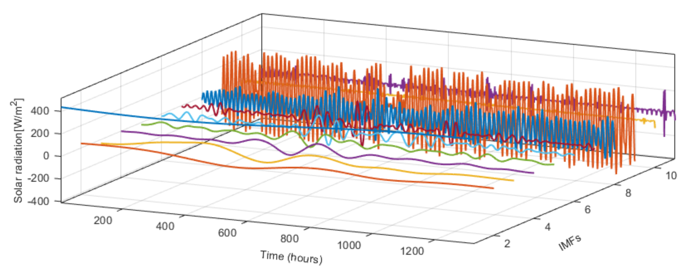
- To reduce the volatility of the original solar data, the non-stationary solar radiation series is divided into several stable sub-series with various scales via the CEEMDAN method. These stable components are simpler than the original series for forecasting, which is beneficial to enhance forecasting accuracy.
- (2)
- According to the inherent features, including periodicity, tendency, and randomness, of the original solar radiation series, a new physical information-based kernel function is designed by using several commonly used kernel functions. A GPR model based on the new physical kernel (PGPR) is constructed. The model PGPR can realize both deterministic and directly probabilistic solar radiation prediction, which is more in line with the actual demand during decision-making.
- (3)
- To handle local optimality and initialization dependence disadvantages of the conjugate gradient (CG) algorithm, widely used for searching the optimal hyper-parameters, BSA is executed to search for the optimum hyperparameters of PGPR.
2. Methodology
2.1. Solar Radiation Prediction Based on ML
2.2. Complete Ensemble Empirical Mode Decomposition with Adaptive Noise
- (1)
- Create a series by adding additional white noise to the original series , where is the noise amplitude;
- (2)
- Execute EMD N times to generate the first components . The final first component is calculated by taking the mean of . The corresponding first residual series is obtained by ;
- (3)
- Decompose the set of noise-added residual series to produce the second ; is the first sub-mode of the . Thus, the final second is calculated by taking the average of ;
- (4)
- The subsequent processes of decomposition are identical to Steps 2–3. After calculating the k-th residual series, the (k + 1)-th mode can be obtained. Continue doing so until the residual series exhibits monotony. The remaining modes of CEEMDAN can be represented mathematically as:
2.3. Gaussian Process Regression with Physical-Based Kernel Function (PGPR)
2.3.1. Basic Principles of Gaussian Process Regression
2.3.2. Covariance Functions and Their Hyperparameters Determination
- (1)
- Squared-Exponential (SE) kernel:
- (2)
- Matern (Ma) 5/2 kernel:
- (3)
- Rational Quadratic (RQ) kernel:
- (4)
- Linear kernel:
- (5)
- Random noise (RN) kernel:where , l is the relevance determination; is the variance and is used to control the degree of local relevance; is the Kronecker’s delta function for x and ; the is called the hyperparameter set of the kernel function.
2.3.3. Physical-Based Kernel Function
2.4. Backtracking Search Optimization Algorithm
2.5. Flowchart of CEEMDAN-BSA-PGPR (CBP) Model
- Step 1: For a nonlinear and nonstationary solar radiation series , employ CEEMDAN to decompose it into a residue, , and several intrinsic mode functions, (IMFs) ;
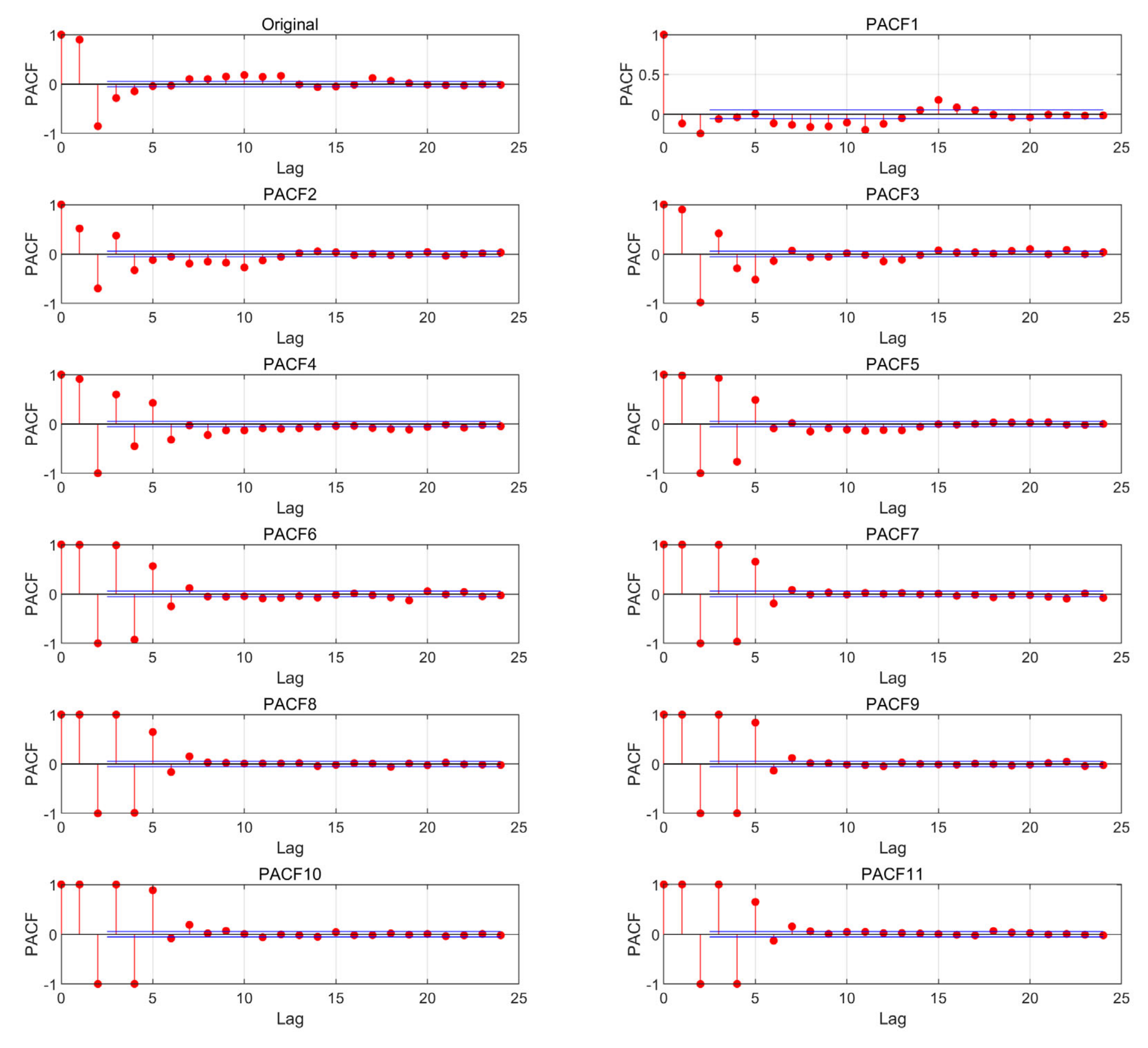
- Step 2: For each component ( or ), apply the PACF to determine suitable input variables;
- Step 3: Based on the selected input, establish PGPR for each component ( or ) and apply the BSA to obtain the best hyperparameters of the PGPR model;
- Step 4: The well-tuned models are utilized separately to do multi-hour-ahead forecasting using the testing dataset for every IMF and the residue;
- Step 5: The final forecasting values of the original solar radiation are obtained by aggregating all prediction results of all the IMFs and the residue.
3. Case Studies
3.1. Data Collection
3.2. Parameter Setting
3.3. Determination of Input Variables
3.4. Performance Criteria
4. Results
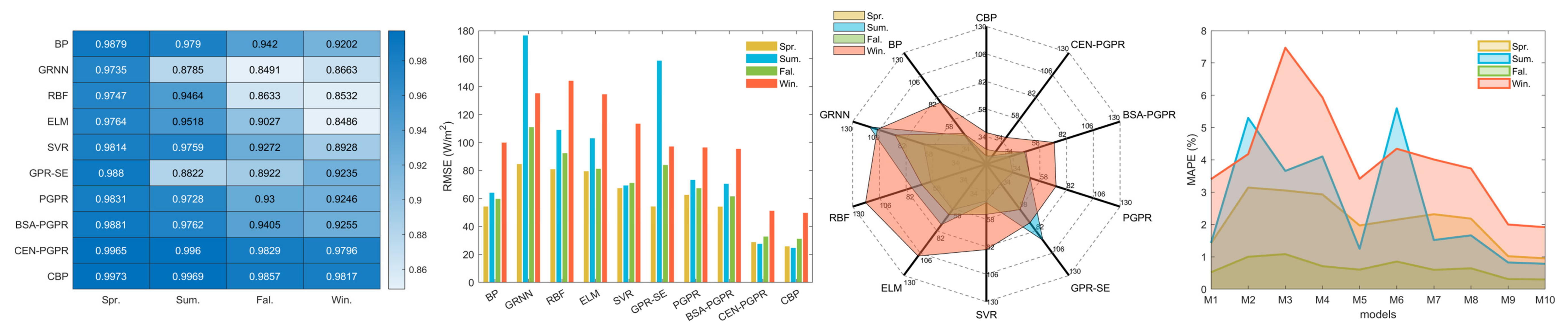
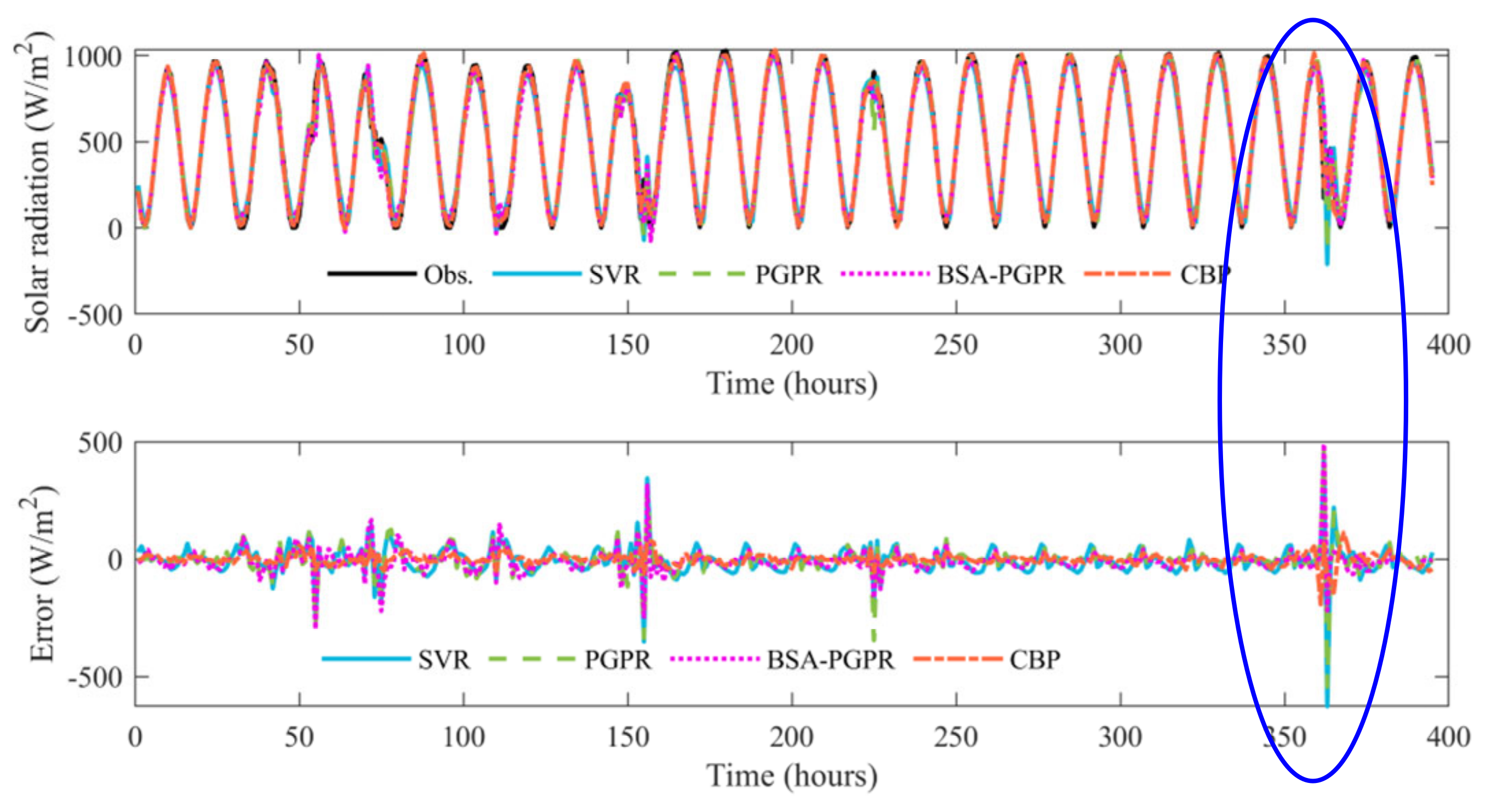
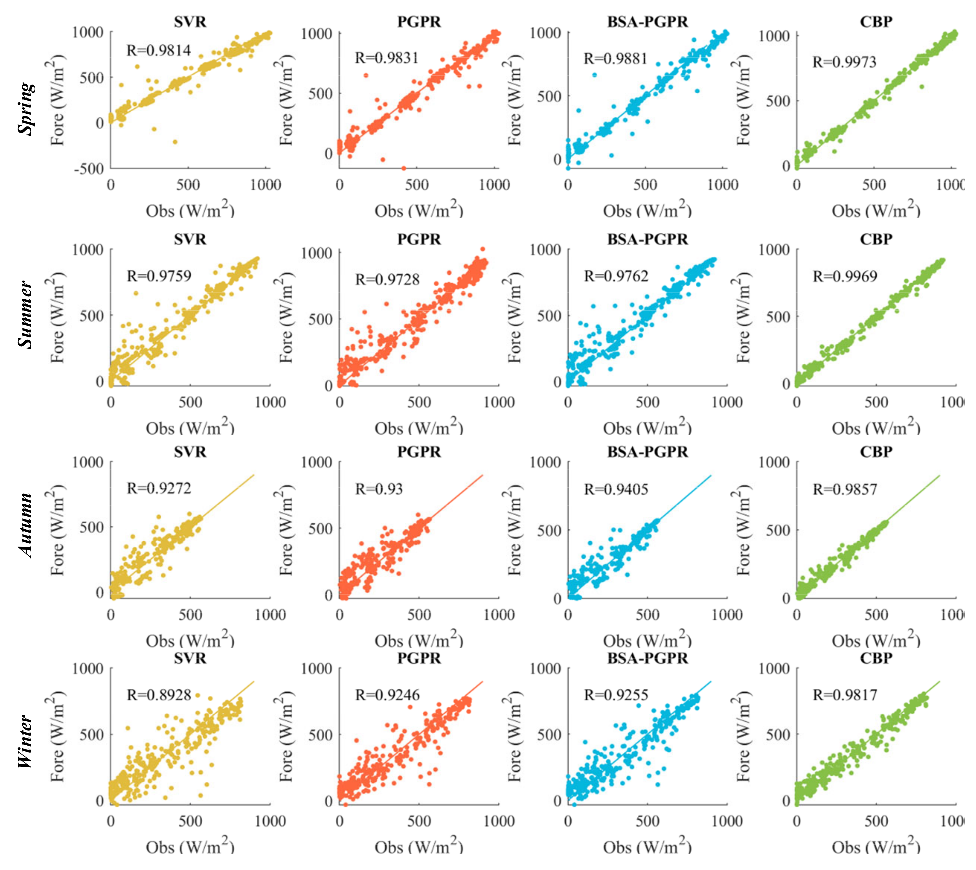
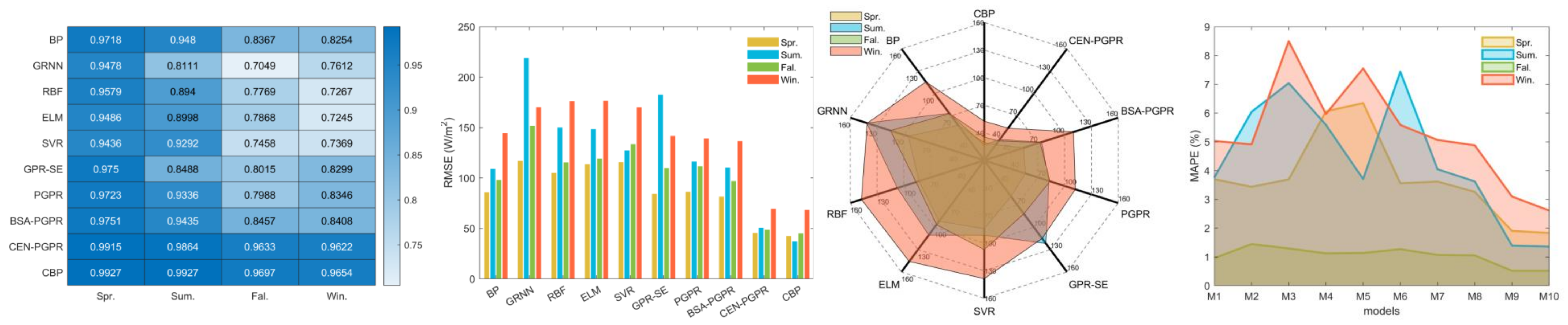
4.1. Results of 1-Hour Ahead Forecasting
4.2. Results of Multi-Hour Ahead Forecasting
5. Discussion
6. Conclusions
- (1)
- The proposed CBP model provided the best results, with the biggest R and lowest RMSE, MAE, and MAPE, which attested to the excellent forecasting ability of the CBP relative to the other comparative models;
- (2)
- The forecasting results produced by the PGPR model are close to or superior to those of the GPR model, indicating that the newly designed kernel function enhances the interpretability of the GPR model while maintaining accuracy;
- (3)
- The proposed PGPR model outperformed many widely used standalone BP, GRNN, RBF, ELM, and SVR models, which revealed the effectiveness of the CBP model relative to other comparative models;
- (4)
- The BSA, applied in searching appropriate hyperparameters of the PGPR, along with the use of CEEMDAN to extract detailed information, can enhance the forecasting ability of CBP. Using BSA alone to optimize PGPR parameters does not always achieve an ideal forecasting performance.
Author Contributions
Funding
Institutional Review Board Statement
Informed Consent Statement
Data Availability Statement
Acknowledgments
Conflicts of Interest
Appendix A. Nomenclature
| AnEn | Analog Ensemble |
| ANN | Artificial neural network |
| AR | Autoregressive |
| ARIMA | Auto-regressive integrated moving average |
| ARMA | Autoregressive moving average |
| BP | Back propagation neural network |
| BSA | Backtracking search optimization algorithm |
| CEEMD | Complementary EEMD |
| CEEMDAN | Complete EEMD with adaptive noise |
| DWT | Discrete wavelet transform |
| EEMD | Ensemble EMD |
| ELM | Extreme learning machine |
| EMD | Empirical mode decomposition |
| EWT | Empirical wavelet transform |
| GA | Genetic algorithms |
| GPR | Gaussian process regression |
| GRNN | Generalized regression neural network |
| IMF | Intrinsic mode function |
| MAE | Mean absolute error |
| MAPE | Mean average percentage error |
| ML | Machine learning |
| NWP | Numerical weather prediction |
| PACF | Partial autocorrelation coefficient function |
| PGPR | Gaussian process regression with physical-based kernel function |
| PSO | Particle swarm optimization |
| R | Pearson’s correlation coefficient |
| RBF | Radial basis function neural network |
| RF | Random forests |
| RMSE | Root mean square error |
| SVM/SVR | Support vector machine/Support vector regression |
| VMD | Variational mode decomposition |
References
- Murdock, H.E.; Gibb, D.; André, T.; Sawin, J.L.; Brown, A.; Ranalder, L.; Collier, U.; Dent, C.; Epp, B.; Hareesh Kumar, C.; et al. Renewables 2021-Global Status Report; UN Environment Programme: Paris, France, 2021. [Google Scholar]
- Liu, Y.; Qin, H.; Zhang, Z.; Pei, S.; Wang, C.; Yu, X.; Jiang, Z.; Zhou, J. Ensemble spatiotemporal forecasting of solar irradiation using variational Bayesian convolutional gate recurrent unit network. Appl. Energy 2019, 253, 113596. [Google Scholar] [CrossRef]
- Sun, S.; Wang, S.; Zhang, G.; Zheng, J. A decomposition-clustering-ensemble learning approach for solar radiation forecasting. Sol. Energy 2018, 163, 189–199. [Google Scholar] [CrossRef]
- Dong, J.; Olama, M.M.; Kuruganti, T.; Melin, A.M.; Djouadi, S.M.; Zhang, Y.; Xue, Y. Novel stochastic methods to predict short-term solar radiation and photovoltaic power. Renew. Energy 2020, 145, 333–346. [Google Scholar] [CrossRef]
- Niu, D.; Wang, K.; Sun, L.; Wu, J.; Xu, X. Short-term photovoltaic power generation forecasting based on random forest feature selection and CEEMD: A case study. Appl. Soft Comput. 2020, 93, 106389. [Google Scholar] [CrossRef]
- Huang, J.; Korolkiewicz, M.; Agrawal, M.; Boland, J. Forecasting solar radiation on an hourly time scale using a Coupled AutoRegressive and Dynamical System (CARDS) model. Sol. Energy 2013, 87, 136–149. [Google Scholar] [CrossRef]
- Sun, H.; Yan, D.; Zhao, N.; Zhou, J. Empirical investigation on modeling solar radiation series with ARMA–GARCH models. Energy Convers. Manag. 2015, 92, 385–395. [Google Scholar] [CrossRef]
- David, M.; Ramahatana, F.; Trombe, P.-J.; Lauret, P. Probabilistic forecasting of the solar irradiance with recursive ARMA and GARCH models. Sol. Energy 2016, 133, 55–72. [Google Scholar] [CrossRef]
- Alsharif, M.H.; Younes, M.K.; Kim, J. Time series ARIMA model for prediction of daily and monthly average global solar radiation: The case study of Seoul, South Korea. Symmetry 2019, 11, 240. [Google Scholar] [CrossRef]
- Ding, S.; Li, R.; Tao, Z. A novel adaptive discrete grey model with time-varying parameters for long-term photovoltaic power generation forecasting. Energy Convers. Manag. 2021, 227, 113644. [Google Scholar] [CrossRef]
- Reddy, K.S.S.; Ranjan, M. Solar resource estimation using artificial neural networks and comparison with other correlation models. Energy Convers. Manag. 2003, 44, 2519–2530. [Google Scholar] [CrossRef]
- Zeng, J.; Qiao, W. Short-term solar power prediction using a support vector machine. Renew. Energy 2013, 52, 118–127. [Google Scholar] [CrossRef]
- Al-Dahidi, S.; Ayadi, O.; Adeeb, J.; Alrbai, M.; Qawasmeh, B.R. Extreme learning machines for solar photovoltaic power predictions. Energies 2018, 11, 2725. [Google Scholar] [CrossRef]
- Zhang, Y.; Cui, N.; Feng, Y.; Gong, D.; Hu, X. Comparison of BP, PSO-BP and statistical models for predicting daily global solar radiation in arid Northwest China. Comput. Electron. Agric. 2019, 164, 104905. [Google Scholar] [CrossRef]
- Yagli, G.M.; Yang, D.; Srinivasan, D. Automatic hourly solar forecasting using machine learning models. Renew. Sustain. Energy Rev. 2019, 105, 487–498. [Google Scholar] [CrossRef]
- Moreira, M.O.; Balestrassi, P.P.; Paiva, A.P.; Ribeiro, P.F.; Bonatto, B.D. Design of experiments using artificial neural network ensemble for photovoltaic generation forecasting. Renew. Sustain. Energy Rev. 2021, 135, 110450. [Google Scholar] [CrossRef]
- Yujing, S.; Fei, W.; Zhao, Z.; Zengqiang, M.; Chun, L.; Bo, W.; Jing, L. Research on Short-Term Module Temperature Prediction Model Based on BP Neural Network for Photovoltaic Power Forecasting. In Proceedings of the 2015 IEEE Power & Energy Society General Meeting, Denver, CO, USA, 26–30 July 2015; IEEE: Piscataway, NJ, USA, 2015; pp. 1–5. [Google Scholar]
- Benali, L.; Notton, G.; Fouilloy, A.; Voyant, C.; Dizene, R. Solar radiation forecasting using artificial neural network and random forest methods: Application to normal beam, horizontal diffuse and global components. Renew. Energy 2019, 132, 871–884. [Google Scholar] [CrossRef]
- Cervone, G.; Clemente-Harding, L.; Alessandrini, S.; Delle Monache, L. Short-term photovoltaic power forecasting using Artificial Neural Networks and an Analog Ensemble. Renew. Energy 2017, 108, 274–286. [Google Scholar] [CrossRef]
- Feng, Y.; Hao, W.; Li, H.; Cui, N.; Gong, D.; Gao, L. Machine learning models to quantify and map daily global solar radiation and photovoltaic power. Renew. Sustain. Energy Rev. 2020, 118, 109393. [Google Scholar] [CrossRef]
- Sun, N.; Zhang, S.; Peng, T.; Zhou, J.; Sun, X. A Composite Uncertainty Forecasting Model for Unstable Time Series: Application of Wind Speed and Streamflow Forecasting. IEEE Access 2020, 8, 209251–209266. [Google Scholar] [CrossRef]
- Sun, N.; Zhang, S.; Peng, T.; Zhang, N.; Zhou, J.; Zhang, H. Multi-Variables-Driven Model Based on Random Forest and Gaussian Process Regression for Monthly Streamflow Forecasting. Water 2022, 14, 1828. [Google Scholar] [CrossRef]
- Zhu, S.; Luo, X.; Xu, Z.; Ye, L. Seasonal streamflow forecasts using mixture-kernel GPR and advanced methods of input variable selection. Hydrol. Res. 2018, 50, 200–214. [Google Scholar] [CrossRef]
- Alali, Y.; Harrou, F.; Sun, Y. Optimized Gaussian Process Regression by Bayesian Optimization to Forecast COVID-19 Spread in India and Brazil: A Comparative Study. In Proceedings of the 2021 International Conference on ICT for Smart Society (ICISS), Bandung, Indonesia, 2–4 August 2021; IEEE: Piscataway, NJ, USA, 2021; pp. 1–6. [Google Scholar]
- Sun, N.; Zhou, J.; Chen, L.; Jia, B.; Tayyab, M.; Peng, T. An adaptive dynamic short-term wind speed forecasting model using secondary decomposition and an improved regularized extreme learning machine. Energy 2018, 165, 939–957. [Google Scholar] [CrossRef]
- Ghimire, S.; Deo, R.C.; Raj, N.; Mi, J. Wavelet-based 3-phase hybrid SVR model trained with satellite-derived predictors, particle swarm optimization and maximum overlap discrete wavelet transform for solar radiation prediction. Renew. Sustain. Energy Rev. 2019, 113, 109247. [Google Scholar] [CrossRef]
- Li, F.-F.; Wang, S.-Y.; Wei, J.-H. Long term rolling prediction model for solar radiation combining empirical mode decomposition (EMD) and artificial neural network (ANN) techniques. J. Renew. Sustain. Energy 2018, 10, 013704. [Google Scholar] [CrossRef]
- Zhang, J.; Zhang, Q.; Li, G.; Wu, J.; Wang, C.; Li, Z. Hybrid Model for Renewable Energy and Load Forecasting Based on Data Mining and EWT. J. Electr. Eng. Technol. 2022, 17, 1517–1532. [Google Scholar] [CrossRef]
- Jiang, Y.; Zheng, L.; Ding, X. Ultra-short-term prediction of photovoltaic output based on an LSTM-ARMA combined model driven by EEMD. J. Renew. Sustain. Energy 2021, 13, 046103. [Google Scholar] [CrossRef]
- Zhang, X.; Wei, Z. A Hybrid Model Based on Principal Component Analysis, Wavelet Transform, and Extreme Learning Machine Optimized by Bat Algorithm for Daily Solar Radiation Forecasting. Sustainability 2019, 11, 4138. [Google Scholar] [CrossRef]
- Torres, M.E.; Colominas, M.A.; Schlotthauer, G.; Flandrin, P. A complete ensemble empirical mode decomposition with adaptive noise. In Proceedings of the 2011 IEEE International Conference on Acoustics, Speech and Signal Processing (ICASSP), Prague, Czech Republic, 22–27 May 2011; IEEE: Piscataway, NJ, USA, 2011; pp. 4144–4147. [Google Scholar]
- Schulz, E.; Speekenbrink, M.; Krause, A. A tutorial on Gaussian process regression: Modelling, exploring, and exploiting functions. J. Math. Psychol. 2018, 85, 1–16. [Google Scholar] [CrossRef]
- Civicioglu, P. Backtracking Search Optimization Algorithm for numerical optimization problems. Appl. Math. Comput. 2013, 219, 8121–8144. [Google Scholar] [CrossRef]
- Zhang, C.; Peng, T.; Nazir, M.S. A novel hybrid approach based on variational heteroscedastic Gaussian process regression for multi-step ahead wind speed forecasting. Int. J. Electr. Power Energy Syst. 2022, 136, 107717. [Google Scholar] [CrossRef]
- Peng, T.; Zhang, C.; Zhou, J.; Nazir, M.S. An integrated framework of Bi-directional long-short term memory (BiLSTM) based on sine cosine algorithm for hourly solar radiation forecasting. Energy 2021, 221, 119887. [Google Scholar] [CrossRef]
- Cao, E.; Bao, T.; Gu, C.; Li, H.; Liu, Y.; Hu, S. A Novel Hybrid Decomposition—Ensemble Prediction Model for Dam Deformation. Appl. Sci. 2020, 10, 5700. [Google Scholar] [CrossRef]


| Datasets | Ave. (W/m2) | Std. (W/m2) | Cv. | Cs. | Max. (W/m2) | Min. (W/m2) | Sample Size | Data Period |
|---|---|---|---|---|---|---|---|---|
| Spring | 526.4 | 340.0 | 0.65 | −0.13 | 1029 | 1 | 1327 | 2017/3/20~2017/6/20 |
| Summer | 483.0 | 326.7 | 0.68 | −0.03 | 1033 | 1 | 1347 | 2017/6/21~2017/9/21 |
| Autumn | 337.4 | 224.3 | 0.66 | 0.08 | 804 | 1 | 998 | 2017/9/22~2017/12/20 |
| Winter | 300.2 | 216.9 | 0.72 | 0.36 | 817 | 1 | 991 | 2017/12/21~2018/3/19 |
| Datasets | Metrics | BP | GRNN | RBF | ELM | SVR | GPR-SE | PGPR | BSA-PGPR | CEN-PGPR | CBP |
|---|---|---|---|---|---|---|---|---|---|---|---|
| Spring | R | 0.9879 | 0.9735 | 0.9747 | 0.9764 | 0.9814 | 0.9880 | 0.9831 | 0.9881 | 0.9965 | 0.9973 |
| RMSE (W/m2) | 54 | 85 | 81 | 79 | 67 | 54 | 63 | 54 | 29 | 26 | |
| MAE (W/m2) | 31 | 66 | 60 | 59 | 42 | 31 | 34 | 31 | 17 | 17 | |
| MAPE (%) | 1.42 | 3.14 | 3.05 | 2.93 | 1.97 | 2.15 | 2.32 | 2.18 | 1.02 | 0.95 | |
| Summer | R | 0.9790 | 0.8785 | 0.9464 | 0.9518 | 0.9759 | 0.8822 | 0.9728 | 0.9762 | 0.9960 | 0.9969 |
| RMSE (W/m2) | 64 | 177 | 109 | 103 | 69 | 159 | 73 | 71 | 28 | 25 | |
| MAE (W/m2) | 41 | 115 | 77 | 75 | 44 | 92 | 49 | 46 | 19 | 17 | |
| MAPE (%) | 1.43 | 5.30 | 3.66 | 4.11 | 1.25 | 5.59 | 1.52 | 1.66 | 0.83 | 0.79 | |
| Fall | R | 0.9420 | 0.8491 | 0.8633 | 0.9027 | 0.9272 | 0.8922 | 0.9300 | 0.9405 | 0.9829 | 0.9857 |
| RMSE (W/m2) | 60 | 111 | 92 | 81 | 71 | 84 | 67 | 62 | 33 | 31 | |
| MAE (W/m2) | 43 | 92 | 68 | 64 | 54 | 59 | 49 | 44 | 24 | 23 | |
| MAPE (%) | 0.52 | 1.00 | 1.08 | 0.71 | 0.60 | 0.85 | 0.60 | 0.64 | 0.31 | 0.30 | |
| Winter | R | 0.9202 | 0.8663 | 0.8532 | 0.8486 | 0.8928 | 0.9235 | 0.9246 | 0.9255 | 0.9796 | 0.9817 |
| RMSE (W/m2) | 100 | 135 | 144 | 134 | 113 | 97 | 96 | 95 | 51 | 50 | |
| MAE (W/m2) | 77 | 108 | 118 | 109 | 85 | 73 | 73 | 71 | 39 | 37 | |
| MAPE (%) | 3.41 | 4.18 | 7.47 | 5.93 | 3.42 | 4.35 | 4.01 | 3.73 | 2.00 | 1.92 |
| Datasets | Metrics | BP | GRNN | RBF | ELM | SVR | GPR-SE | PGPR | BSA-PGPR | CEN-PGPR | CBP |
|---|---|---|---|---|---|---|---|---|---|---|---|
| Spring | R | 0.9718 | 0.9478 | 0.9579 | 0.9486 | 0.9436 | 0.9750 | 0.9723 | 0.9751 | 0.9915 | 0.9927 |
| RMSE (W/m2) | 86 | 117 | 105 | 114 | 116 | 84 | 86 | 81 | 46 | 43 | |
| MAE (W/m2) | 57 | 95 | 83 | 92 | 84 | 59 | 56 | 54 | 31 | 29 | |
| MAPE (%) | 3.70 | 3.44 | 3.69 | 6.06 | 6.34 | 3.56 | 3.62 | 3.26 | 1.90 | 1.83 | |
| Summer | R | 0.9480 | 0.8111 | 0.8940 | 0.8998 | 0.9292 | 0.8488 | 0.9336 | 0.9435 | 0.9864 | 0.9927 |
| RMSE (W/m2) | 109 | 219 | 150 | 149 | 127 | 183 | 116 | 110 | 51 | 37 | |
| MAE (W/m2) | 73 | 141 | 107 | 111 | 91 | 122 | 83 | 74 | 38 | 27 | |
| MAPE (%) | 3.76 | 6.04 | 7.04 | 5.59 | 3.71 | 7.43 | 4.04 | 3.62 | 1.39 | 1.36 | |
| Fall | R | 0.8367 | 0.7049 | 0.7769 | 0.7868 | 0.7458 | 0.8015 | 0.7988 | 0.8457 | 0.9633 | 0.9697 |
| RMSE (W/m2) | 98 | 152 | 116 | 119 | 134 | 110 | 112 | 97 | 49 | 45 | |
| MAE (W/m2) | 73 | 115 | 86 | 96 | 107 | 82 | 84 | 73 | 36 | 35 | |
| MAPE (%) | 0.96 | 1.44 | 1.29 | 1.12 | 1.14 | 1.27 | 1.07 | 1.05 | 0.52 | 0.52 | |
| Winter | R | 0.8254 | 0.7612 | 0.7267 | 0.7245 | 0.7369 | 0.8299 | 0.8346 | 0.8408 | 0.9622 | 0.9654 |
| RMSE (W/m2) | 145 | 170 | 176 | 177 | 170 | 142 | 139 | 137 | 70 | 68 | |
| MAE (W/m2) | 116 | 141 | 147 | 146 | 139 | 115 | 112 | 110 | 53 | 53 | |
| MAPE (%) | 5.03 | 4.91 | 8.50 | 5.97 | 7.55 | 5.59 | 5.06 | 4.88 | 3.10 | 2.61 |
| Datasets | Metrics | BP | GRNN | RBF | ELM | SVR | GPR-SE | PGPR | BSA-PGPR | CEN-PGPR | CBP |
|---|---|---|---|---|---|---|---|---|---|---|---|
| Spring | R | 0.9497 | 0.9242 | 0.9383 | 0.9173 | 0.9040 | 0.9571 | 0.9587 | 0.9585 | 0.9805 | 0.9813 |
| RMSE (W/m2) | 112 | 139 | 132 | 139 | 147 | 112 | 110 | 106 | 68 | 67 | |
| MAE (W/m2) | 78 | 116 | 108 | 117 | 117 | 85 | 84 | 78 | 48 | 47 | |
| MAPE (%) | 2.27 | 3.58 | 4.33 | 5.89 | 6.31 | 2.97 | 3.00 | 3.08 | 2.46 | 1.95 | |
| Summer | R | 0.9046 | 0.7885 | 0.8486 | 0.8460 | 0.8589 | 0.8152 | 0.8806 | 0.9037 | 0.9719 | 0.9845 |
| RMSE (W/m2) | 144 | 236 | 184 | 182 | 179 | 207 | 160 | 147 | 73 | 54 | |
| MAE (W/m2) | 100 | 158 | 135 | 141 | 138 | 145 | 117 | 105 | 56 | 40 | |
| MAPE (%) | 6.13 | 7.29 | 8.49 | 7.54 | 7.52 | 8.07 | 6.77 | 6.52 | 2.30 | 1.90 | |
| Fall | R | 0.7693 | 0.6666 | 0.7617 | 0.6781 | 0.5326 | 0.7781 | 0.6881 | 0.7924 | 0.9314 | 0.9437 |
| RMSE (W/m2) | 115 | 152 | 116 | 141 | 175 | 113 | 137 | 110 | 67 | 61 | |
| MAE (W/m2) | 88 | 119 | 91 | 118 | 148 | 85 | 107 | 83 | 50 | 48 | |
| MAPE (%) | 0.88 | 1.40 | 1.21 | 1.37 | 1.67 | 1.19 | 1.37 | 1.12 | 0.76 | 0.70 | |
| Winter | R | 0.7159 | 0.6372 | 0.6747 | 0.6224 | 0.5339 | 0.7258 | 0.7341 | 0.7406 | 0.9268 | 0.9346 |
| RMSE (W/m2) | 177 | 198 | 191 | 202 | 219 | 173 | 171 | 169 | 97 | 93 | |
| MAE (W/m2) | 144 | 168 | 163 | 167 | 180 | 144 | 141 | 139 | 79 | 76 | |
| MAPE (%) | 6.08 | 6.61 | 8.13 | 6.03 | 9.08 | 6.11 | 5.27 | 4.69 | 5.03 | 3.53 |
| Datasets | Improvements (%) | CEN-PGPR vs. PGPR | CBP vs. BSA-PGPR | ||||
|---|---|---|---|---|---|---|---|
| 1-hour | 2-hour | 3-hour | 1-hour | 2-hour | 3-hour | ||
| Spring | PR | 1.37 | 1.97 | 2.27 | 0.93 | 1.80 | 2.37 |
| PRMSE | 54.09 | 47.24 | 37.84 | 52.49 | 47.82 | 37.04 | |
| PMAE | 47.85 | 44.63 | 42.30 | 44.75 | 45.69 | 39.26 | |
| PMAPE | 56.06 | 47.44 | 17.87 | 56.32 | 43.84 | 36.61 | |
| Summer | PR | 2.39 | 5.66 | 10.37 | 2.13 | 5.22 | 8.94 |
| PRMSE | 62.41 | 56.42 | 54.76 | 65.00 | 66.38 | 62.96 | |
| PMAE | 61.17 | 54.03 | 52.31 | 62.37 | 63.96 | 62.10 | |
| PMAPE | 45.72 | 65.58 | 66.00 | 52.80 | 62.57 | 70.86 | |
| Fall | PR | 5.69 | 20.60 | 35.35 | 4.81 | 14.67 | 19.10 |
| PRMSE | 51.32 | 56.45 | 51.32 | 49.32 | 53.54 | 44.63 | |
| PMAE | 51.85 | 56.81 | 53.36 | 48.52 | 51.28 | 42.56 | |
| PMAPE | 47.99 | 51.74 | 44.65 | 53.53 | 50.87 | 37.16 | |
| Winter | PR | 5.96 | 15.30 | 26.25 | 6.08 | 14.82 | 26.20 |
| PRMSE | 46.91 | 50.00 | 43.13 | 47.93 | 49.94 | 45.00 | |
| PMAE | 46.67 | 52.41 | 44.30 | 47.30 | 52.15 | 45.04 | |
| PMAPE | 50.16 | 38.81 | 4.59 | 48.68 | 46.46 | 24.76 | |
| Datasets | Improvements (%) | BSA-PGPR vs. PGPR | CBP vs. CEN-PGPR | ||||
|---|---|---|---|---|---|---|---|
| 1-hour | 2-hour | 3-hour | 1-hour | 2-hour | 3-hour | ||
| Spring | PR | 0.51 | 0.29 | −0.02 | 0.07 | 0.12 | 0.08 |
| PRMSE | 13.58 | 5.54 | 3.17 | 11.8 | 7.05 | 1.95 | |
| PMAE | 8.02 | 4.02 | 7.45 | 2.63 | 6.22 | 2.65 | |
| PMAPE | 5.93 | 9.89 | −2.68 | 6.95 | 3.86 | 26.2 | |
| Summer | PR | 0.35 | 1.06 | 2.62 | 0.09 | 0.64 | 1.28 |
| PRMSE | 3.81 | 5.06 | 8.56 | 11.66 | 36.52 | 33.59 | |
| PMAE | 7.62 | 10.04 | 9.77 | 11.71 | 41.78 | 39.45 | |
| PMAPE | −9.43 | 10.40 | 3.81 | 5.1 | 2.65 | 21.31 | |
| Fall | PR | 1.13 | 5.87 | 15.15 | 0.29 | 0.66 | 1.3 |
| PRMSE | 8.60 | 13.15 | 19.81 | 5.09 | 7.95 | 9.63 | |
| PMAE | 10.33 | 13.29 | 22.64 | 4.3 | 2.24 | 4.95 | |
| PMAPE | −8.02 | 1.67 | 18.82 | 3.61 | 0.11 | 8.51 | |
| Winter | PR | 0.10 | 0.74 | 0.88 | 0.21 | 0.33 | 0.83 |
| PRMSE | 1.04 | 1.84 | 0.92 | 3.01 | 1.73 | 4.35 | |
| PMAE | 2.13 | 1.86 | 1.78 | 3.39 | 1.34 | 3.18 | |
| PMAPE | 6.94 | 3.66 | 11.07 | 4.36 | 18.63 | 42.6 | |
Publisher’s Note: MDPI stays neutral with regard to jurisdictional claims in published maps and institutional affiliations. |
© 2022 by the authors. Licensee MDPI, Basel, Switzerland. This article is an open access article distributed under the terms and conditions of the Creative Commons Attribution (CC BY) license (https://creativecommons.org/licenses/by/4.0/).
Share and Cite
Sun, N.; Zhang, N.; Zhang, S.; Peng, T.; Jiang, W.; Ji, J.; Hao, X. An Integrated Framework Based on an Improved Gaussian Process Regression and Decomposition Technique for Hourly Solar Radiation Forecasting. Sustainability 2022, 14, 15298. https://doi.org/10.3390/su142215298
Sun N, Zhang N, Zhang S, Peng T, Jiang W, Ji J, Hao X. An Integrated Framework Based on an Improved Gaussian Process Regression and Decomposition Technique for Hourly Solar Radiation Forecasting. Sustainability. 2022; 14(22):15298. https://doi.org/10.3390/su142215298
Chicago/Turabian StyleSun, Na, Nan Zhang, Shuai Zhang, Tian Peng, Wei Jiang, Jie Ji, and Xiangmiao Hao. 2022. "An Integrated Framework Based on an Improved Gaussian Process Regression and Decomposition Technique for Hourly Solar Radiation Forecasting" Sustainability 14, no. 22: 15298. https://doi.org/10.3390/su142215298
APA StyleSun, N., Zhang, N., Zhang, S., Peng, T., Jiang, W., Ji, J., & Hao, X. (2022). An Integrated Framework Based on an Improved Gaussian Process Regression and Decomposition Technique for Hourly Solar Radiation Forecasting. Sustainability, 14(22), 15298. https://doi.org/10.3390/su142215298