Article

Time Series Data Modeling Using Advanced Machine Learning and AutoML

1
Yogananda School of AI, Computer and Data Science, Shoolini University, Solan 173229, India
2
Maharishi Markandeshwar Engineering College, Maharishi Markandeshwar (Deemed to be University), Mullana, Ambala 133207, India
3
School of Creative Technologies, University of Bolton, Bolton BL3 5AB, UK
*
Authors to whom correspondence should be addressed.
Sustainability 2022, 14(22), 15292; https://doi.org/10.3390/su142215292
Submission received: 24 September 2022 / Revised: 4 November 2022 / Accepted: 7 November 2022 / Published: 17 November 2022

Abstract

:
A prominent area of data analytics is “timeseries modeling” where it is possible to forecast future values for the same variable using previous data. Numerous usage examples, including the economy, the weather, stock prices, and the development of a corporation, demonstrate its significance. Experiments with time series forecasting utilizing machine learning (ML), deep learning (DL), and AutoML are conducted in this paper. Its primary contribution consists of addressing the forecasting problem by experimenting with additional ML and DL models and AutoML frameworks and expanding the AutoML experimental knowledge. In addition, it contributes by breaking down barriers found in past experimental studies in this field by using more sophisticated methods. The datasets this empirical research utilized were secondary quantitative data of the real prices of the currently most used cryptocurrencies. We found that AutoML for timeseries is still in the development stage and necessitates more study to be a viable solution since it was unable to outperform manually designed ML and DL models. The demonstrated approaches may be utilized as a baseline for predicting timeseries data.

1. Introduction

Research on time series analytics is demonstrated in past research works [1,2] with a rich background and its pivotal importance trended recently with the growth of data volumes [3,4,5]. Due to the significance of the field, tools that are reliable, scalable, and accurate in forecasting are in high demand. The last decade has seen a spike in the number of suggested forecasting models [6,7,8]. Recent developments should eventually provide the possibility to efficiently model this type of data. However, the ambiguity of timeseries data makes modeling it a difficult task. ML and DL models generally can perform well in the task [9] but require experience to set up the model and adjust its hyperparameters [10]. Moreover, in sophisticated models, the number of hyperparameters to adjust becomes large and necessitates laborious effort. Moreover, the designed model might become vulnerable to data drift [11,12] where the properties of the independent variable change over time, which is a common issue in timeseries data [13,14]. AutoML strives to solve the former two problems by automatically finding an appropriate model and adjusting its hyperparameters in light of the data [15]. A variety of AutoML frameworks are available for forecasting timeseries data, for example, EvalML [16], AutoKeras [17], and others [18,19].This paper represents the results and findings of experiments in the utilization of AutoML to tackle the data drift in timeseries data in providing higher-accuracy predictions.
Hamayel et al. (2021) [20] proposed three variants of Recurrent Neural Networks (RNNs) including Gated Recurrent Unit (GRU), Long Sort Term Memory (LSTM), and Bi-Directional LSTM (Bi-LSTM) to forecast the prices of several cryptocurrencies. Among the models, Bi-LSTM achieved the worst, with GRU achieving the best. Awoke et al. (2021) [21] developed LSTM and GRU for Bitcoin forecasting and found that GRU-based models are superior at predicting extremely volatile time series. Several AutoML comparative studies [22,23,24,25] compared different AutoML frameworks on standard tasks. The studies showed either a large variance or no significant variance across models. However, in simple classification tasks, AutoML frameworks did not substantially outperform conventional models or humans [26]. Paldino et al. (2021) [26] tested four AutoML frameworks (AutoGluon, H2O, TPOT, and Auto-Sklearn) against a benchmark of traditional forecasting algorithms (naive, exponential smoothing, and Holt-Winter’s) on a range of timeseries forecasting tasks. Their findings demonstrated that AutoML approaches are still immature for timeseries forecasting problems. However, mainly, the models did not give concern to the data drift problem and aimed to have high accuracy on the testing dataset. Alsharef et al. [27] reviewed different ML and AutoML solutions that can be utilized in forecasting and recommended the use of the EvalML AutoML framework to solve the problem of forecasting concerning data drift issues. Other comparative studies [9,28] evaluated different techniques to solve the problem of forecasting having promising results. In addition, non-financial applications of timeseries analysis found a place in most recent research. For example, product sales [29] and weather [30]. Daniela et al. [31] researched the process of data analysis and generation of prediction models of energy consumption in smart buildings. Huseyin et al. [32] proposed a hybrid model for streamflow forecasting due to the necessity of water management after the growth in water consumption.
This paper includes an experimental study on the effectiveness of various approaches that can be used for the problem of forecasting timeseries data including RNN, GRU, LSTM, Independent RNN (IndRNN), Auto-Regressive (AR), Moving Average (MA), Auto-Regressive Moving Average (ARMA), Auto-Regressive Integrated Moving Average (ARIMA), and Linear Regression (LR). Additionally, two AutoML frameworks—EvalML and Auto-Keras—were utilized to automatically search for the best prediction models concerning the data. The datasets were quantitative and included historical timeseries data of real prices of the cryptocurrencies Ethereum and Bitcoin gathered from a reputable bulletin [33,34]. With MSEs of 298 and 287, respectively, IndRNN was shown to have a stronger prediction potential than the other currently used approaches. Additionally, deep learning models outperformed linear models in terms of prediction accuracy. For AutoML, the best models with the Ethereum dataset, according to AutoML frameworks EvalML and Auto-Keras, were Random Forest and GRU, respectively, with MSEs of 762 and 414. The best models with the Bitcoin dataset, on the other hand, were Decision Tree Regressor and LSTM, with MSEs of 693 and 376.We concluded that AutoML for timeseries modeling is currently in development, and it necessitates hard work from researchers to evolve.
Due to the characteristics of time series data such as being structured and small in size, the models did not require high infrastructure and had a relatively low computation cost compared with 2d and 3d data that require high computation costs, for example. The experiments of this work did not consider the computational cost of the models. No model required more than 45 min to train (training ARIMA on BTC-ETH dataset with parameters [2,6,7] on a normal laptop device was the slowest operation). The experiments were performed on the processor “Intel Core i5-7200U CPU” with “8192 MB RAM Memory”.
This paper contributed in:
  • Performing a comparative experimental study on different ML and DL models and AutoML frameworks.
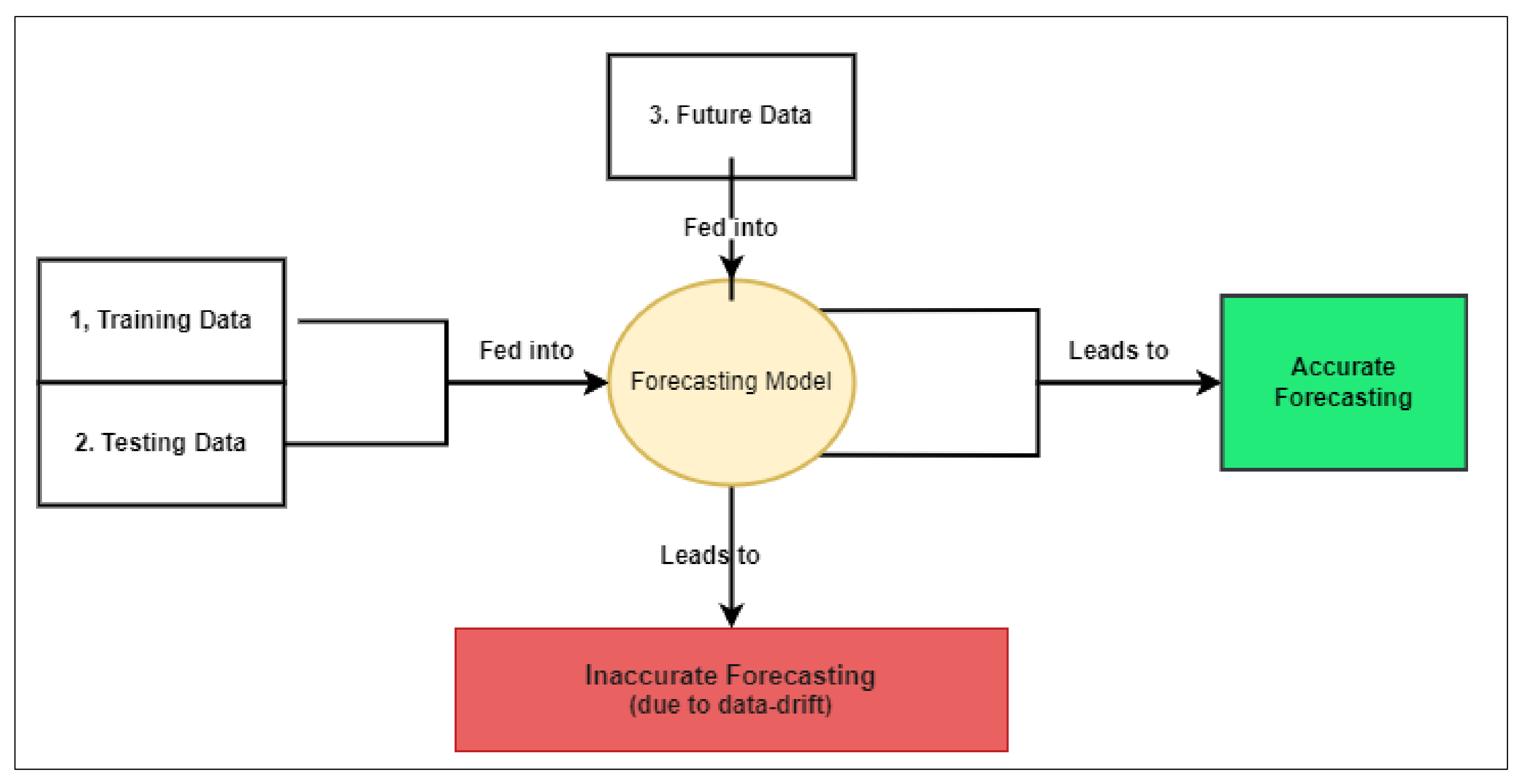
  • Defining the problem of data drift and investigating the ability of the automation in ML to tackle it.
  • Representing a contribution to establishing the use of theory-based methods such as AutoML in experimental studies.
  • Adding to the growing body of literature by elaborating the problem of data drift and elaborating the AutoML concept where this work can serve as an example for researchers to conduct empirical or review studies on ML and AutoML.
  • This experimental work can be applied in extended time series domains and enables the widening of the same research domain with other data features.
  • This work provided a comprehensive analysis of cryptocurrency data in an area where data significantly vary (from time to time and cryptocurrency to another).

2. Literature Review

2.1. TimeSeries Forecasting

Massive volumes of timeseries data are now accessible, providing businesses and professionals with new potential for data mining and decision making. Linear models [35,36] for timeseries forecasting [37] have been extensively used for a while, and many scientists still use them since they are accurate and straightforward to understand. However, recent breakthroughs in machine learning research showed that neural networks can be more effective models to forecast timeseries [38] as they achieve higher accuracy [9]. However, these linear and deep learning methods need in-depth domain expertise for data pre-processing, feature selection, and hyperparameter tuning in order to successfully complete a forecasting task [39]. Since it is difficult to find researchers with both machine learning and domain knowledge, using time series forecasting techniques may be a tedious task for organizations conducting research in different domains [40]. The need for frameworks to automate the ML process has increased as a result of this gap [40]. Automated machine learning (AutoML) provides solutions to build and run machine learning pipelines while minimizing human involvement [41].Analyzing data with limited human involvement has become an interesting topic for researchers and industries [42,43,44]. However, establishing a mechanism that automates the whole ML process for forecasting is not yet a developed area of study, and also contains limitations and peculiarities that should be handled in special ways [26].
Examples from the plethora of studies in timeseries forecasting in the sustainability domain and its applications include the following examples.
Oana et al. [45] conducted a study on economic applications on the basis of the Eurostat database [46]. The study was built around the problem of the circular economy over data with features that cover all areas of interest (production and consumption, waste management, secondary raw materials, and competitiveness and innovation). For each selected feature, experimented time series prediction models were able to reveal accurate forecasts with respect to different time horizons. The limitation concerned the length of the data series available in the Eurostat database (only since 2000) making possible the establishment of a limited predictive horizon.
Muhammad et al. [47] conducted a study on economic applications focused on forecasting the data of the inflation and exchange rates from 1989 to 2020 in a generalizable use case, using different ML algorithms such as KNNs, polynomial regression, ANNs, and SVM. The data set was split into a training set (from 1989 to 2018) and a testing set(from 2019 to 2020). For forecasting inflation rates based on error prediction, the test set showed that the polynomial regression and ANN methods outperformed SVM and KNN. On the other hand, forecasting the exchange rate, SVM RBF outperformed KNN, polynomial regression, and ANNs. The results showed that the parameter setting of all ML algorithms is also important.
Jintian et al. [48] conducted a study on economy that investigated the impacts of democracy, environmental regulations, renewable energy, globalization, and economic growth on “ecological footprints” [49], which is a method to measure human demand on natural capital, i.e., the quantity of nature it takes to support people or economy, from 1990 to 2018, in a generalizable use case example of N-11 (Next Eleven) countries. They applied the cross-sectional autoregressive distributed lags (CS-ARDL) methods. The results showed that environmental regulation significantly mitigates ecological footprint, while economic growth escalates ecological footprints. Additionally, all selected features were contributing factors to environmental quality.
Antonio et al. [50] conducted a study on climate change that analyzed in a generalizable use case the regularity of monthly rainfall timeseries during the period 1953 to 2012, recorded at 133 measuring stations well-distributed across the study area. They used the sample entropy (SampEn) method, by calculating SampEn values in 10 year sliding windows for the whole series and by applying statistical tests for two 30-year subperiods. The study was able to provide detailed spatiotemporal analysis of rainfall regime, to distinguish among different rainfall regimes, and to identify climatic phenomena.
Eyad et al. [51] carried out a study on climate change aimed to analyze hydrological variability by conducting an intensive analysis of extreme events, under dry and wet conditions. They utilized four meteorological stations selected to provide daily rainfall rates based on a dataset of recorded data periods of rainfall ranging from 24 years to 70 years. They mentioned that the performance of any model on a different storm event could be different based on the recording interval and, therefore, the results will change accordingly.
This work adds to the plethora of timeseries analytics in sustainability applications, providing a generalizable empirical study on ML and AutoML techniques that can be utilized for modeling.

2.2. Machine Learning

The moving average (MA) model is a simple straightforward approach where the predicted value at time t + 1 is equal to the average (mean) of the earlier values up to time t. Despite linear models’ underlying simplicity, some of them, such as ARIMA, have been shown to be very accurate and efficient predictors [9,28,52]. ANN is designed to analyze and learn from many different unidentified inputs. Because ANNs are non-linear, they may be used to compute intricate relationships between input and output [28,53]. For this reason, it can be utilized to effectively predict timeseries volatile data. ANN contains parameters and hyperparameters [54] that significantly control the processes of learning. The parameters and hyperparameters affect the whole process of predicting and determining their values and significantly influence the model behavior. These parameters should be selected or initialized carefully by the researcher intending to achieve satisfactory outcomes. Most machine learning algorithms require extensive domain knowledge, pre-processing, feature selection, and hyperparameter optimization to be able to solve a forecasting task with a satisfying result [39]. Analysts with both machine learning and domain expertise are relatively rare, which makes engagement with time series forecasting methods expensive for organizations. Moreover, machine learning models are vulnerable to data drift [11,12] where the properties of the independent variable change over time. Therefore, an pre-designed model might not be able to forecast future data accurately.

2.3. Data Drift Problem

After a machine learning model is placed into production and users start using it, one of the main concerns of data scientists is whether the model will still capture the pattern of new incoming data and whether it will efficiently continue to capture the pattern of newly incoming data as it was functioning during its design phase. Data drift is defined as the changes to data structure, semantics, and infrastructure that are unforeseen and undocumented as a consequence of modern data architectures [55]. In other words, data driftis a type of model drift that occurs when the characteristics of the independent input variables change. Data drift examples include seasonal variations in data, shifts in customer preferences, exposure to new items, etc. This issue is common when working with time series data which is volatile and vulnerable to sudden change. The following Figure 1 illustrates the problem of data drift.

2.4. Automated Machine Learning

The term “AutoML” refers to the automation of machine learning tasks such that no (or very little) manual work is necessary [56]. With AutoML, non-experts had the opportunity to use machine learning methods to tackle a particular problem without needing any previous technical or domain expertise [57]. Most methods of AutoML aim to completely automate the model selection, hyperparameter optimization, and feature selection processes. [58]. Previously, many methods and tactics only addressed a portion of this AutoML process and in recent years, various completely automated methods have emerged.
The AutoML automated approach underlines several steps until the selected model becomes ready to perform forecasting:
  • Model Selection: The objective of model selection, given a collection of ML models and a dataset, is to identify ML models with the greatest accuracy when trained on the dataset. AutoML aims to determine the model that best fits the data without human involvement, iterating over many models to be trained on the same input data and selecting the model with the best performance [27,59].
  • Hyperparameter Optimization (HPO): Setting and adjusting hyperparameters appropriately will often result in a model with enhanced performance. Additionally, research has shown that an appropriate choice of hyper-parameters considerably improves the performance of models in comparison with the default model settings [60,61]. HPO is an important technique in machine learning that became essential owing to the upscaling of neural networks to improve accuracy. Due to the upscaling of neural networks for improved accuracy, a potential set of hyperparameter values becomes essential, necessitating that researchers have experience with neural networks when manually setting the hyperparameter [27]. Bayesian Optimization [62] and Random Search [63] are examples of strategies for automated HPO.
  • Feature Engineering: This is another step that can be achieved by AutoML which is tedious and repetitive when performed manually [27].
Recently, many frameworks have been proposed that combine all three former steps of AutoML. For example: AutoKeras [17], EvalML [16], AutoGluon [64], Auto-Weka [65], Auto-PyTorch [66], and others.
EvalML [16] is an open-source AutoML framework that automatically executes feature selection, model selection, hyper-parameter optimization, etc. It uses random forest classifier/regressor for feature selection and Bayesian optimization to optimize its pipeline hyperparameters. It builds and optimizes ML pipelines depending on an objective function parameter, e.g., MSE in case of timeseries forecasting. It supports various supervised ML problem types, including regression, classification, time series regression, and time series classification. In this work, we set the problem type as “timeseries regression”. In our previous paper [27], we compared different AutoML frameworks and we gave the recommendation to use EvalML for timeseries forecasting. This work will use it to auto search for the optimal models and auto optimize concerning the data.
AutoKeras [17] is an AutoML system depending on the widely used Keras API. Amongst other equivalent AutoML systems, Auto-Keras emphasizes deep learning over basic ML models. It uses a special Neural Architecture Search (NAS) algorithm for searching over neural architectures to best address a modeling job. Since AutoKeras uses an efficient algorithm for auto search in advanced optimal models, this work will use the this AutoKeras AutoML system.
We concluded by combining our current empirical study and our previous literature study [27] of different AutoML steps and frameworks and determined that the computational cost of AutoML depends on the search space and the searching algorithm. In other words, efficiency depends on the initial space and algorithm set by the pipeline designer. Therefore, some manual work is still required. Some frameworks, such as EvalML, select the search spaces depending on the problem type; in the case of time series, it searches within architectures used frequently for time series and this minimizes the search space of the model selection, HPO, and feature engineering resulting in a computationally efficient pipeline. Other frameworks, such as AuroKeras, search within more sophisticated architectures such as neural networks where it runs each model for a certain number of epochs to estimate its accuracy with given data resulting in a lower computationally efficient but more accurate pipeline. However, overall, the computational cost for time series data analysis is not a big concern compared with larger data such as3rd images, for example, since it has a low volume, clear structure, less complex model architecture, and lower number of parameters.

3. Experimental Work

3.1. Data and Pre-Processing

3.1.1. Data Collection

Two datasets were employed for training and testing the proposed models [33,34].
  • The datasets were collected from a reliable bulletin (Yahoo Finance).
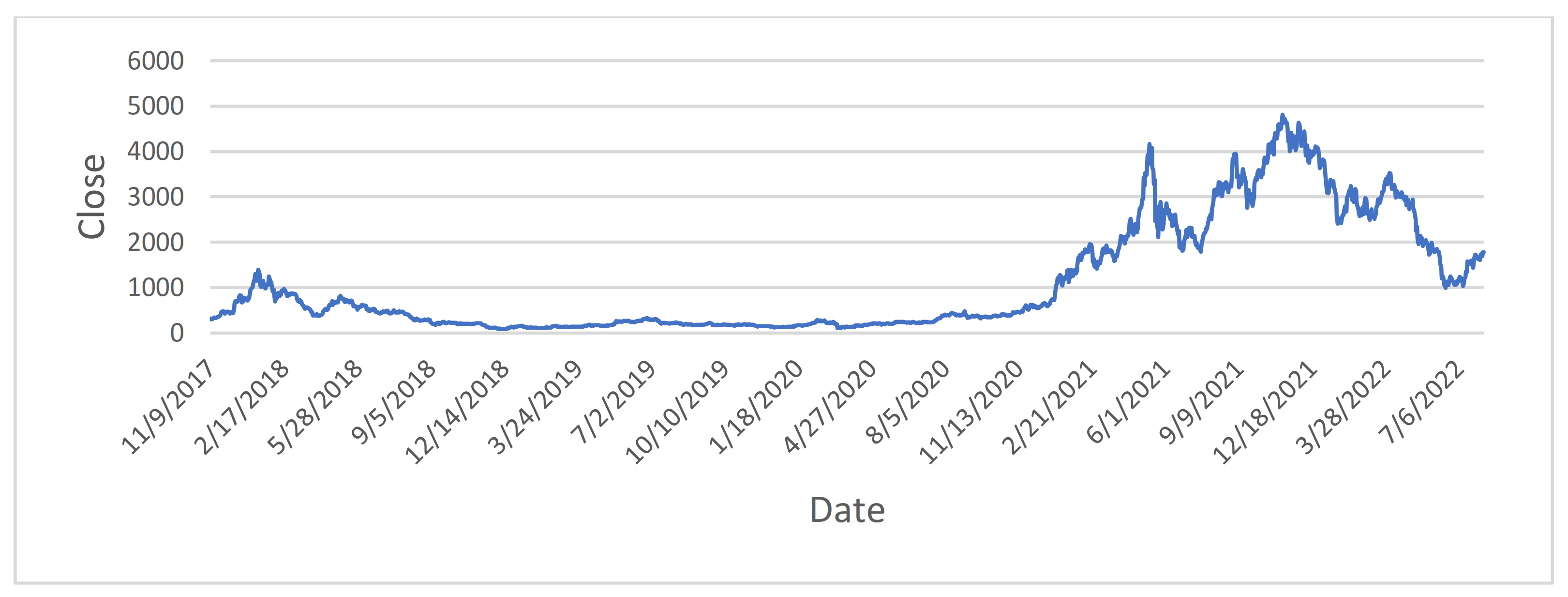
  • The first dataset contained the daily Ethereum cryptocurrency prices in U.S. Dollars (ETH-USD) from 8 July 2015 to 9 August 2022 with 2590 observations.
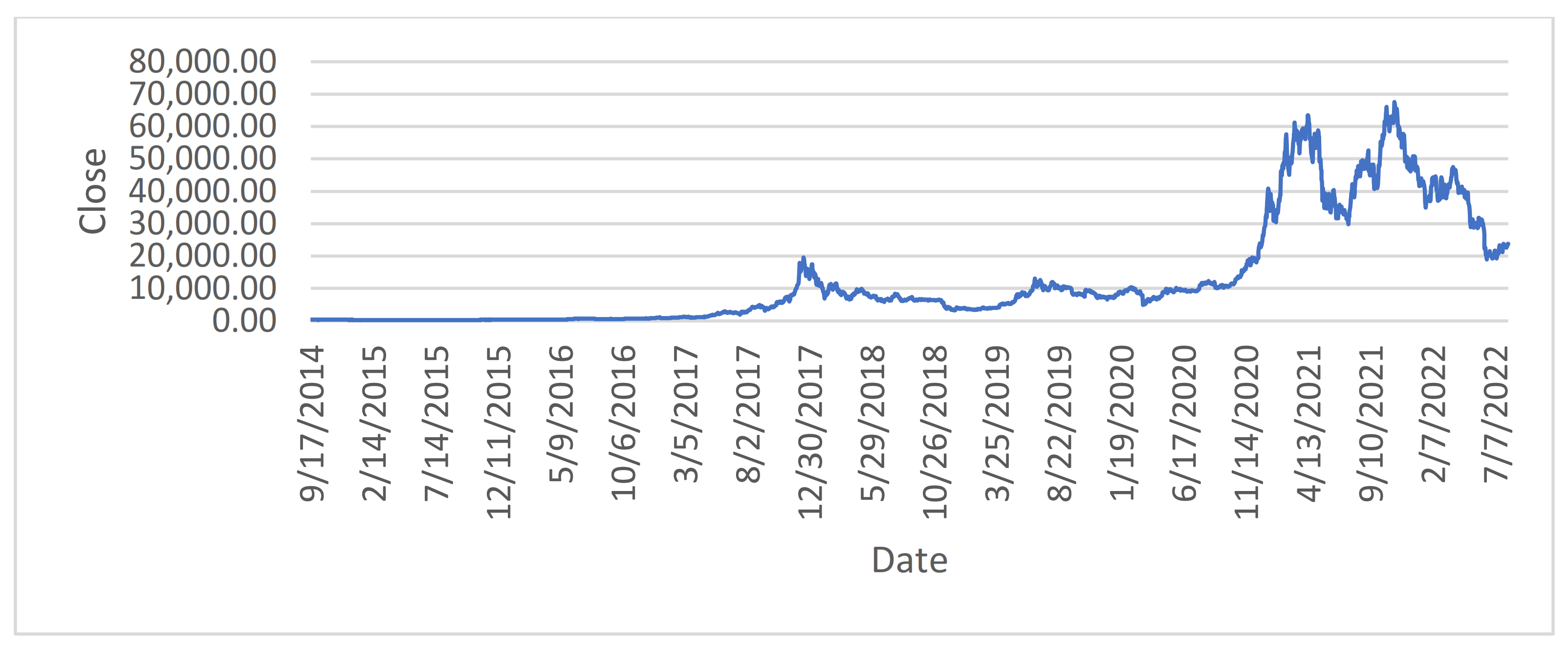
  • The 2nd data set contained the daily Bitcoin cryptocurrency prices in U.S. Dollars (BTC-USD) from 17 September 2014 to 9 August 2022 with 2886 observations.
  • Each dataset contained mainly the following features: date (date of observation taken), Close price, Open price, High price, Low price, Volume, and Adj Close price.
The study used the Date and Close features for analysis since the closing price is the most important feature of the data and it is the basic data that is used in the analysis of the stock market [67].

3.1.2. Data Visualization

A chart showing the fluctuations in the 1st dataset (Ethereum close prices in USD historical data) starting from 2017 is provided in the following Figure 2.
We observed that the data had minimal fluctuations until the end of2020 when a spike in price and the following fluctuations can be seen.
A chart showing the fluctuations in the 2nd dataset (Bitcoin close prices in USD historical data) starting from 2015 is provided in the following Figure 3.
We observed that the data had mild fluctuations until early 2021 when a trough in price followed by an immediate spike and later fluctuations can be seen.
As we can conclude from the charts, while the prices of both cryptocurrencies are highly volatile, Ethereum is more stable to an extent. On the other hand, Bitcoin is an older cryptocurrency with a larger volume of historical data available.
As a part of understanding the data, ACF and PACF plots were drawn for both datasets to determine the best parameters to be used with AR, MA, ARMA, and ARIMA models.
ACF [68] is a function that gives values of autocorrelation of any series with its lagged values. ACF plot describes how highly the present value of a series is connected to its past values.
PACF [68] is a partial autocorrelation function where instead of finding correlations of the present with lags, it finds a correlation of the residuals (which remains after removing the effects which are already explained by the earlier lag(s)). In PACF, we correlate the “parts” of y t and y t 3 that are not predicted by y t 1 and y t 2 .
The following Figure 4, Figure 5, Figure 6 and Figure 7, show ACF and PACF plots for the datasets used in this empirical study.
Figure 4 shows the ACF plot for the 1st database, ETH-USD:
Figure 5 shows the PACF plot for the 1st database, ETH-USD:
Figure 6 shows the ACF plot for the 2nd database, BTC-USD:
Figure 7 shows the PACF plot for the 2nd database, BTC-USD:

3.1.3. Data Pre-Processing

The following Table 1 illustrates data quality properties.
The cleaning process included filling the missed values by approximating each missed value by its corresponding previous value. In other words, the missed price of a certain day is considered the same price as the previous days. The data format was unified by converting strings to numbers, handling symbols such as “$”, and converting all to a unified number format. Data values were rounded into an integer number. For example, a value of 222.5 was rounded to 222 to facilitate calculation. The closing price is the most important feature of the data. It is the basic data that is used in the analysis of the stock market [67]. We selected the “Close” price as a target for modeling and “Date” and historical “Close” prices as an input.

3.2. Methodology

  • This work used a combination of machine learning models and AutoML frameworks that auto-find and tune optimal ML models to solve the problems of forecasting time series and data drift. The machine learning models included: LR, AR, MA, ARMA, ARIMA, RNN, GRU, LSTM, and IndRNN. The AutoML frameworks included: EvalML and Auto-Keras.
  • The datasets included: Ethereum cryptocurrency prices in U.S. Dollars (ETH-USD) from 2015 to 2022 and Bitcoin cryptocurrency prices in U.S. Dollars (BTC-USD) from 2014 to 2022.
  • The MSE and MAE scores were used as evaluation metrics to compare the models’ efficiency, which is the mean of the squared errors. The larger this metric is the larger the error indicating that the model is less accurate. The units of MSE and MAE are the same as the unit of measurement for the quantity, which is being estimated, U.S. Dollars in our case.
  • The programming language used for implementation was Python.
  • After data pre-processing and feature selection, this work experimented with 9 machine learning models to model the timeseries data and then experimented with two AutoML frameworks to model the same.

3.2.1. Machine Learning

The 9 machine learning models used in this work included 5 linear models: MA, AR, ARMA, LR, and ARIMA, and 4 deep learning models: RNN, GRU, LSTM, and IndRNN. The linear models were:
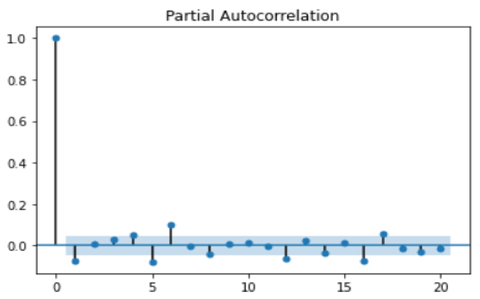
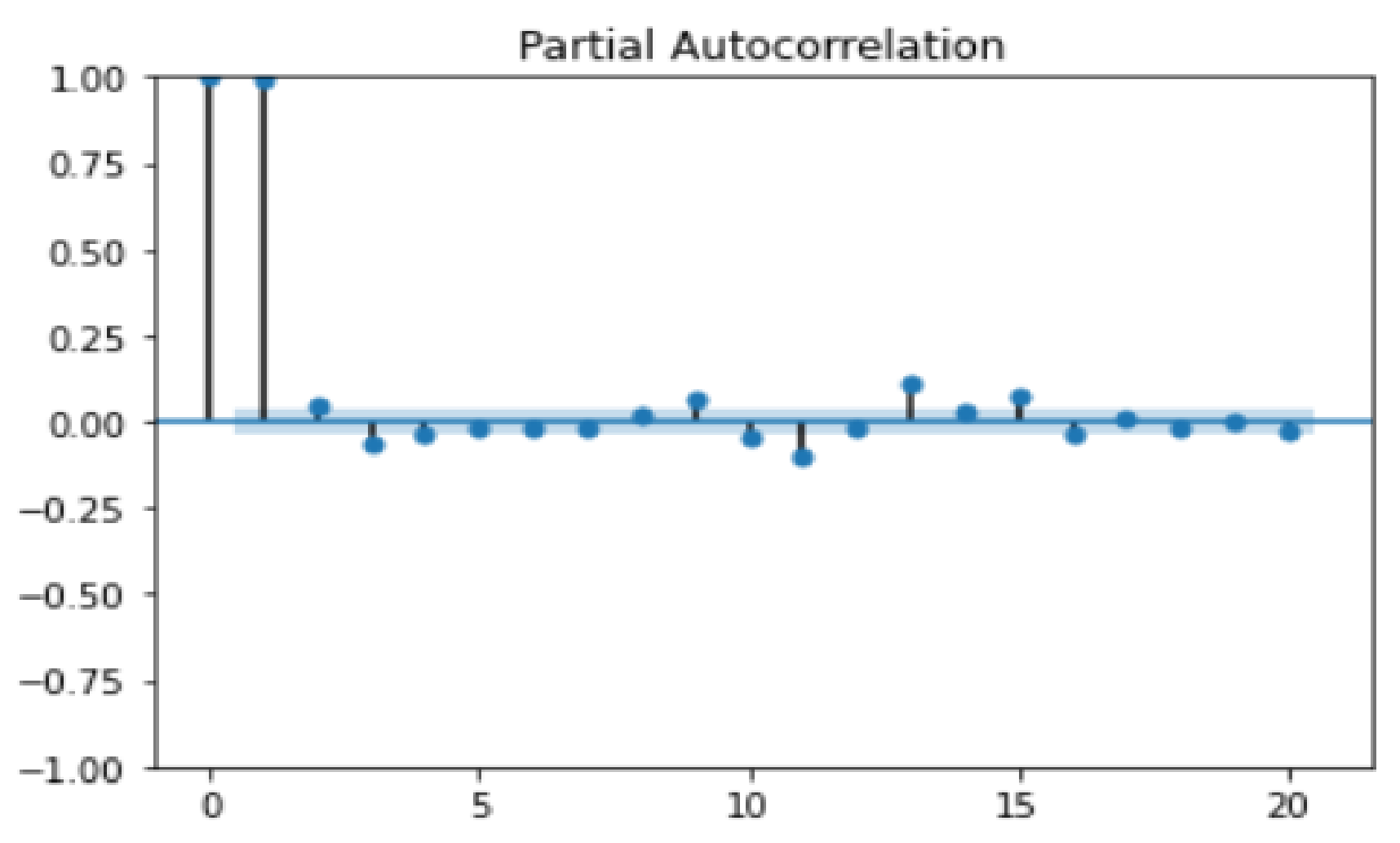
  • Auto-Regressive (AR) [27,69] with the parameters: p = 12 on the 1st dataset and p = 12 on the 2nd dataset. These parameters were set using PACF plots [68] that can determine the partial autocorrelation between a value and its proceedings in a time series. The higher the partial autocorrelation, the higher the impact on prediction.
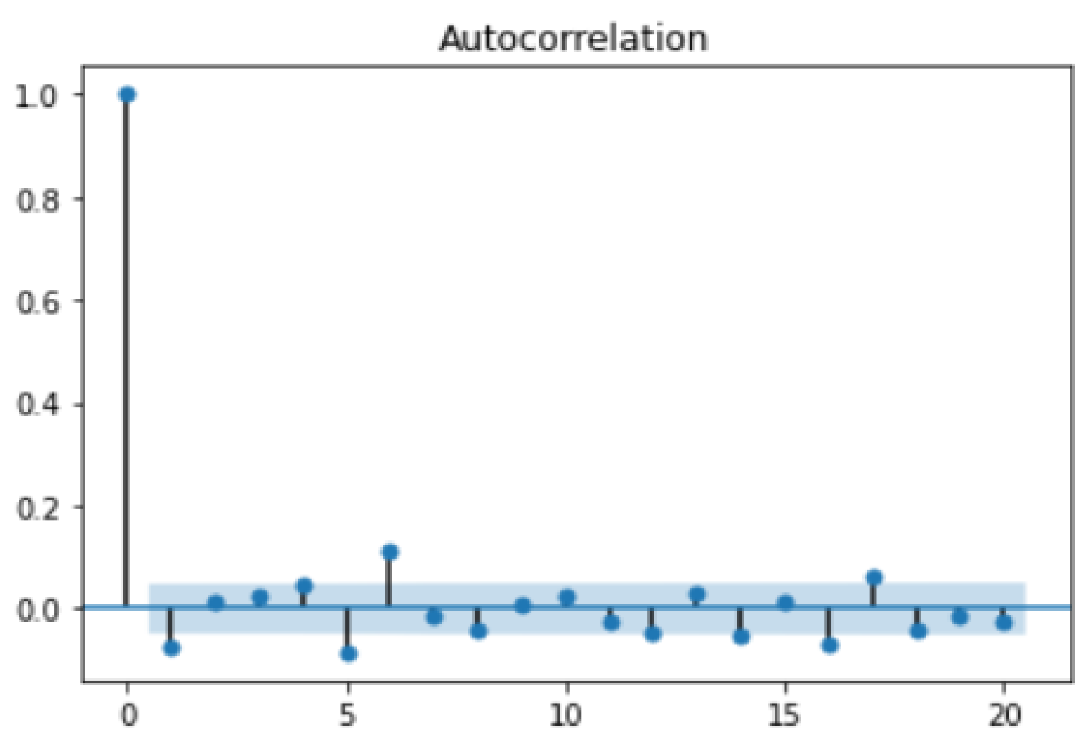
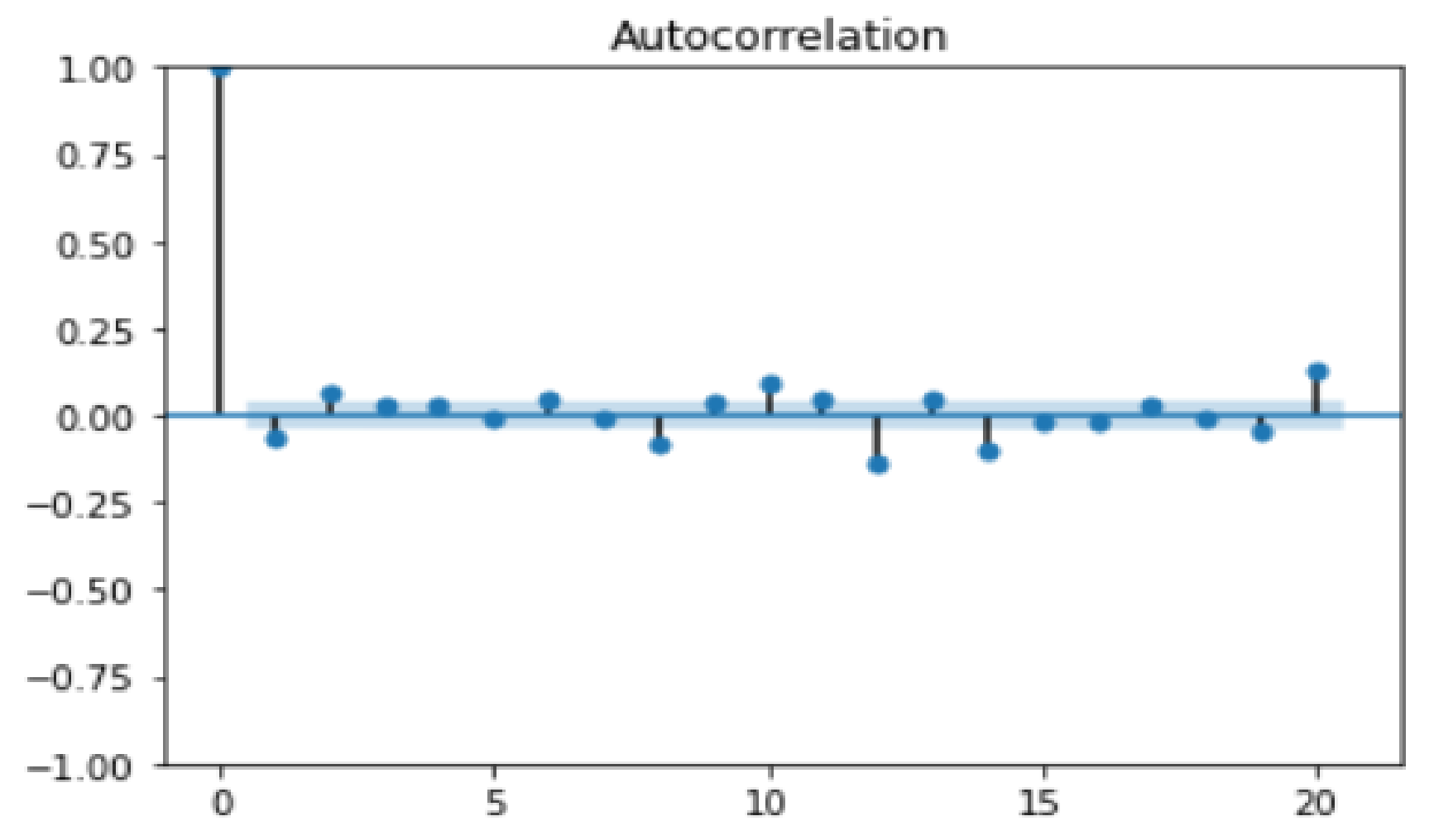
  • Moving Average (MA) [70] with the parameters: q = 14 on the 1st dataset and q = 14 on the 2nd dataset. These parameters were set using ACF plots [68] that can determine the autocorrelation between a value and its proceedings in a time series. The higher the autocorrelation, the higher the impact on prediction.
  • ARMA [71] with the parameters: p = 12, q = 14 on both the 1st dataset and 2nd dataset. These parameters were set using both ACF and PACF plots that can determine, combined, the optimal order for the ARMA model parameters.
  • ARIMA [72] with the parameters: p = 7, d = 1, and q = 7 on the 1st dataset and p = 6, d = 2, and q = 7 on the 2nd dataset. These parameters were set using the grid search optimization algorithm [23] which automatically discovers the optimal order for an ARIMA model.
  • Linear Regression (LR) [73] where all training data points (closing prices) for each dataset were used to draw a fitting line of the data using the ordinary least squares method.
The deep learning models were RNN, GRU, LSTM, and IndRNN. These deep learning models followed state-of-the-art architecture, and the problem configuration of all the deep learning models was as follows:
  • Forecast horizon: 5;
  • Max delay (lookback): 20;
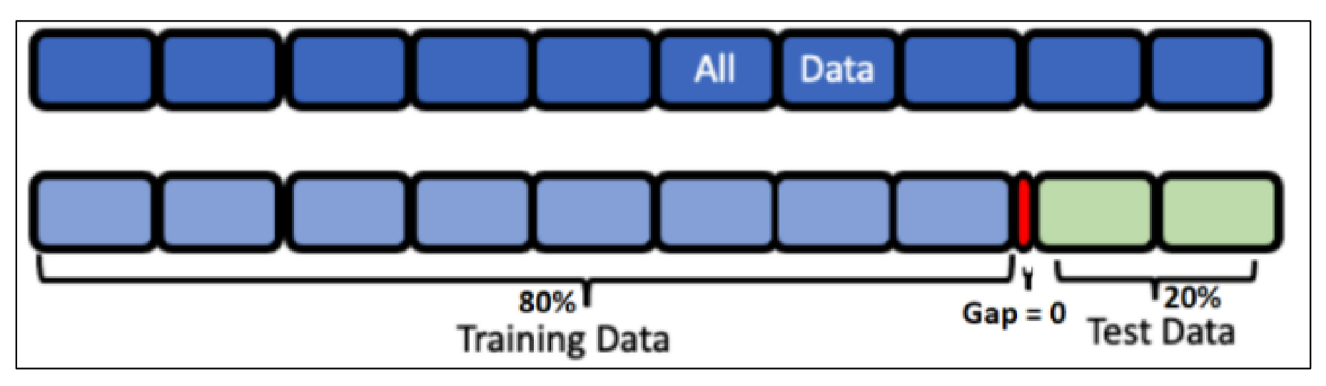
  • Gap: 0;
  • Batch size: 20 for each deep learning model;
  • Number of hidden layers: 3, for each deep learning model;
  • Learning rate: 0.001, for each deep learning model;
  • Time index: Date.
where:
  • Forecast horizon: The number of future periods we are attempting to forecast. In this example, we want to forecast prices for the next 5 days, hence the value is 5. According to [74], predicting a long horizon is not an easy task and choosing a shorter horizon such as 5 is more useful.
  • Max delay: The maximum number of past values to investigate from the present value in order to construct forecasting input features. Increasing the max delay (look-back period) might result in lesser error rates, but would imply a higher dimensional input and hence increased complexity [75]. In our example, a sliding window method was used, where the previous 20 values were used to predict the next 5 values.
  • Gap: The number of periods that pass between the end of the training set and the beginning of the test set. Throughout our example, the gap is zero since we are trying to forecast the prices for the following five days using the data as it is “today”. However, if we were to forecast prices for the next Monday through Sunday using data from the prior Friday, the difference would be 2 (Saturday and Sunday separate Monday from Friday).
  • Time index: The column of the training set, having the date of the corresponding observation.

3.2.2. AutoML

This work used 2 AutoML frameworks to automatically find optimal models and tune them concerning the data. These frameworks were EvalML and Auto-Keras.
EvalML is an AutoML framework for creating, optimizing, and evaluating machine learning pipelines based on domain-specific objective functions. In this work, our goal is to forecast future values for the time series by utilizing its historical values. EvalML time series functionality is designed for this purpose. We used EvalML with the same problem configuration of our state-of-the-art deep learning models: {Forecast horizon: 5, Max delay: 20, Gap: 0, Time index: Date} for the same reasons we selected them with state-of-the-art DL models. The same datasets were loaded: ETH-USD and BTC-USD. First, we cleaned the data following the same procedure with ML and DL models. Second, we used the DefaultDataChecks of EvalML to check the health of data where EvalML accepts a Pandas data frame as an input, which can also run type inference on this data directly.
Sustainability 14 15292 i001
These default data checks have a built-in functionality to validate data by checking for errors and recommending a preprocessing action. In our case, this automated preprocessing was recommended to apply log-normal transformation on the data as a normalizing and preprocessing action. For this reason, the lognormal transformation was applied to the dataset. Third, we used the AutoSplit functionality of EvalML to split the data into training and testing datasets depending on the problem type (time series regression in this case) and the problem configurations (forecast horizon, max delay, gap, and time index).
We performed this action which was recommended by the AutoML framework, EvalML, having DefaultDataChecks [76] which is a collection of data checks defined to check for some of the most common data issues.
After that, we performed the AutoSplit functionality of EvalML which splits the data into training and testing data depending on the problem type and timeseries problem configurations.
Sustainability 14 15292 i002
The AutoSplit divided each dataset into 80% of the samples as training data and 20% of them as testing data with cross validation as shown in the following Figure 8.
We applied AutoML techniques to let the machine determine the best prediction models. We followed the same window slide method where the data of the previous 20 days were used to predict the following 5 days’ data. We used the AutoML search function of the EvalML framework. We passed the training data, the type of problem, and the number of batches. It returned the top models that fit the training data.
Sustainability 14 15292 i003
This gave us the best 5 models to be used in forecasting that were: Random Forest, Extra Trees, LightGBM, XGBoost, and Decision Tree on the 1st dataset and Decision Tree, Elastic Net, XGBoost, Random Forest, and Extra Trees on the 2nd dataset.
AutoKeras is a widely used AutoML framework based on Keras. It uses a network morphism Neural Architecture Search (NAS), which is a method for model selection, to automatically search and tune deep neural networks. Many NAS approaches require a large number of searched networks to reach good performance. Moreover, many of them train each neural network in the search scope from scratch, which makes the searching process very slow. However, Auto-Keras uses network morphism NAS methodology that keeps the functionality of a neural network while changing its neural architecture and this could be helpful as it enables more efficient training during the search [17]. Using AutoKeras to search within advanced neural network architectures on both datasets, we configured the auto search within 30 different models and trained each model for 30 epochs to determine its efficiency with a batch size of 20, with the same problem configuration: {Forecast horizon: 5, Max delay: 20, Gap: 0, Time index: Date}.
Sustainability 14 15292 i004
This gave us the best model to be used in forecasting which was a GRU-based architecture on the 1st dataset and an LSTM-based architecture on the 2nd dataset.

4. Result Analysis

4.1. Machine Learning

This work experimented with nine different machine learning models including five linear models: LR, MA, AR, ARMA, and ARIMA, and four deep learning models: RNN, GRU, LSTM, and IndRNN. After applying the experiments on the preprocessed data using the former models, the tested mean squared errors (MSEs) and mean absolute errors (MAEs) resulting for each model on each dataset are provided in the following Table 2.
As Bitcoin is an older cryptocurrency with larger historical data available, the same models worked and achieved better accuracy than Ethereum which is newer and has less available data. Bitcoin was more predictable due to the availability of data and the large dataset used for training. IndRNN showed the best efficiency since it addresses the problems of gradient vanishing and exploding. LSTM showed the 2nd best efficiency due to its capability to process longer sequences than RNN and GRU due to its memory. ARIMA showed good efficiency due to its good configuration generated automatically using GridSearch.

4.2. EvalML

The ranking of the models when applying EvalML autosearch on the Ethereum dataset is shown in the following Table 3.
The former table showed the ranking of models with their respective cross-validation MSE scores. The top five models were as follows:
  • Random Forest;
  • Extra Trees;
  • Light Gradient Boosting Machine (LightGBM);
  • eXtreme Gradient Boosting (XGBoost);
  • Decision Tree Regressor.
All the models contained an imputer for replacing missing data, a timeseries featurizer, and a date–time featurization component. By training the former models on the ETH-USD training dataset and testing on the ETH-USD testing dataset, we obtained an MSE as a test score for each model as shown in the following Table 4.
The previous results showed that the best model suggested with EvalML achieved an MSE of 762 on ETH-USD dataset which is higher than the MSE achieved by many of the manually designed deep learning models indicating that it is not optimal. This can infer that the EvalML autosearch did not yet outperform the traditional deep learning.
The ranking of models when applying EvalML autosearch on the Bitcoin dataset is shown in the following Table 5.
The former table showed the ranking of models with their respective cross validation score. The top five models were as follows:
  • Decision Tree Regressor;
  • Elastic Net Regressor;
  • eXtreme Gradient Boosting (XGBoost);
  • Random Forest Regressor;
  • Extra Trees Regressor.
All the models contained an imputer for replacing missing data, a timeseries featurizer, and a date–time featurization component. By training the former models on the BTC-USD training dataset and testing on the BTC-USD testing dataset, we obtained an MSE as the test score for each model as shown in the following Table 6.
The previous results showed that the best model suggested with EvalML achieved an MSE of 693 on the BTC-USD dataset which is lower than the MSE achieved by many of the manually designed deep learning models, indicating better efficiency; however, it was not optimal since it yielded higher MSE than LSTM and IndRNN. This can infer that EvalML autosearch did not yet outperform the traditional machine learning and deep learning models.

4.3. AutoKeras

Using AutoKeras to search within advanced neural network architectures on the ETH-USD dataset, we configured the auto search within 30 different models and trained for 30 epochs on each model (from its search scope) to determine its efficiency with a batch size of 20, with the same problem configuration. The autosearch concluded that the best architecture that fits the data included the following layers:
  • Input layer;
  • GRU layer;
  • GRU layer;
  • GRU layer;
  • Dropout layer;
  • Dense layer;
The above layers had the following hyperparameters illustrated in Table 7.
After training the resulting model for 200 epochs with the same configuration ({’time_index’: ‘Date’, ‘max_delay’: 20, ‘gap’: 0, ‘forecast_horizon’: 5}) and testing it, we obtained a test MSE of 414 on the first dataset (ETH-USD),which means higher accuracy than many of the manually designed models and higher accuracy than EvalML suggested models; however, it was also not optimal.
Using AutoKeras to search within advanced neural network architectures on the BTC-USD dataset, we configured the auto search within 30 different models and trained for 30 epochs on each model (from its search scope) to determine its efficiency with a batch size of 20, with the same problem configuration. The auto search concluded that the best architecture that fits the data included the following layers:
  • Input layer;
  • Bidirectional LSTM layer;
  • Bidirectional LSTM layer;
  • Dropout layer;
  • Dense layer.
The above layers had the following hyperparameters illustrated in Table 8.
After training the resulting model for 200 epochs with the same configuration ({time_index: Date, max_delay: 20, gap: 0, forecast_horizon: 5}) and testing it, we obtained a testing MSE of 376 on the first dataset (ETH-USD), which means higher accuracy than many of our proposed models and higher accuracy than EvalML suggested models; however, it was also not optimal.

5. Conclusions

Timeseries modeling, which forecasts future values for the time series using previous data on the same variable, is found to have significance in data modeling. The many cases in which it is utilized, including those involving the economy, the atmosphere, asset prices, and capital investment data, demonstrate its significance. The efficiency of different ML, DL, and AutoML methodologies that might be employed to solve this issue was experimentally studied in this research concerning the data drift problem that was challenging in previous studies. The datasets were quantitative historical timeseries data gathered from a reliable bulletin on the prices of the cryptocurrencies Ethereum and Bitcoin. Based on our experiments, we came to the conclusion that AutoML for timeseries is still at the development level and necessitates further study to be a feasible approach. The demonstrated techniques may be employed as a starting point for predicting timeseries data with satisfying accuracy. This study did not provide an alternative AutoML pipeline to overcome the current problems. A high-level scope experimental analysis of further AutoML methods that tests numerous frameworks with various model selection and optimization techniques will be part of future work. In addition, a new AutoML framework with pipelines for timeseries forecasting will be designed and implemented to overcome the current automated forecasting limitations. Moreover, comparative study needs to go one step further and determine whether this difference is significant (for predictive purposes) or simply due to the specific choice of data values in the sample, whereas depending on performance metrics for comparing is not always sufficient. Further research can use the Diebold–Mariano test [77] to determine whether the two forecasts are significantly different.

Author Contributions

Conceptualization, A.A. and S.; methodology, A.A. and S.; software, A.A. and K.K.; validation, K.K.; formal analysis, A.A. and S.; investigation, K.K.; resources, S.; data curation, S.; writing—original draft preparation, S. and K. K.; writing—review and editing, K.K. and C.I.; visualization, C. I.; supervision, C. I. All authors have read and agreed to the published version of the manuscript.

Funding

This research received no external funding.

Institutional Review Board Statement

Not applicable.

Informed Consent Statement

Not applicable.

Data Availability Statement

Data available in a publicly accessible repository that does not issue DOIs Data available in a publicly accessible repository that does not issue DOIs at: https://finance.yahoo.com/quote/ETH-USD/history/?guccounter=1 (accessed on 10 August 2022), https://finance.yahoo.com/quote/BTC-USD/history/?guccounter= (accessed on 10 August 2022).

Conflicts of Interest

The authors declare no conflict of interest.

References

  1. De Gooijer, J.G.; Hyndman, R.J. 25 Years of IIF Time Series Forecasting: A Selective Review; Tinbergen Institute Discussion Paper, No. 05-068/4; Tinbergen Institute: Amsterdam, The Netherlands, 2005; pp. 5–68. [Google Scholar]
  2. Clements, M.P.; Franses, P.H.; Swanson, N.R. Forecasting economic and financial time-series with non-linear models. Int. J. Forecast. 2004, 20, 169–183. [Google Scholar] [CrossRef] [Green Version]
  3. Cowpertwait, P.S.P.; Metcalfe, A. V Introductory Time Series with R; Springer: Berlin/Heidelberg, Germany, 2009; ISBN 0387886982. [Google Scholar]
  4. Parray, I.R.; Khurana, S.S.; Kumar, M.; Altalbe, A.A. Time series data analysis of stock price movement using machine learning techniques. Soft Comput. 2020, 24, 16509–16517. [Google Scholar] [CrossRef]
  5. Frick, T.; Glüge, S.; Rahimi, A.; Benini, L.; Brunschwiler, T. Explainable Deep Learning for Medical Time Series Data. In Proceedings of the International Conference on Wireless Mobile Communication and Healthcare, Virtual Event, 18–19 December 2020; pp. 244–256. [Google Scholar]
  6. Shen, Z.; Zhang, Y.; Lu, J.; Xu, J.; Xiao, G. A novel time series forecasting model with deep learning. Neurocomputing 2020, 396, 302–313. [Google Scholar] [CrossRef]
  7. Livieris, I.E.; Pintelas, E.; Pintelas, P. A CNN–LSTM model for gold price time-series forecasting. Neural Comput. Appl. 2020, 32, 17351–17360. [Google Scholar] [CrossRef]
  8. Du, S.; Li, T.; Yang, Y.; Horng, S.-J. Multivariate time series forecasting via attention-based encoder–decoder framework. Neurocomputing 2020, 388, 269–279. [Google Scholar] [CrossRef]
  9. Alsharef, A.; Bhuyan, P.; Ray, A. Predicting Stock Market Prices Using Fine-Tuned IndRNN. Int. J. Innov. Technol. Explor. Eng. 2020, 9, 309–315. [Google Scholar] [CrossRef]
  10. Marc Claesen, B.D.M. Hyperparameter Search in Machine Learning. In Proceedings of the MIC 2015: The XI Metaheuristics International Conference, Agadir, Morocco, 7–10 June 2015. [Google Scholar]
  11. Ackerman, S.; Raz, O.; Zalmanovici, M.; Zlotnick, A. Automatically detecting data drift in machine learning classifiers. arXiv 2021, arXiv:2111.05672. [Google Scholar]
  12. Ackerman, S.; Farchi, E.; Raz, O.; Zalmanovici, M.; Dube, P. Detection of data drift and outliers affecting machine learning model performance over time. arXiv 2020, arXiv:2012.09258. [Google Scholar]
  13. Rahmani, K.; Thapa, R.; Tsou, P.; Chetty, S.C.; Barnes, G.; Lam, C.; Tso, C.F. Assessing the effects of data drift on the performance of machine learning models used in clinical sepsis prediction. medRxiv 2022. [Google Scholar] [CrossRef]
  14. Fields, T.; Hsieh, G.; Chenou, J. Mitigating drift in time series data with noise augmentation. In Proceedings of the 2019 International Conference on Computational Science and Computational Intelligence (CSCI), Las Vegas, NV, USA, 5–7 December 2019; pp. 227–230. [Google Scholar]
  15. Tornede, T.; Tornede, A.; Wever, M.; Hüllermeier, E. Coevolution of remaining useful lifetime estimation pipelines for automated predictive maintenance. In Proceedings of the Genetic and Evolutionary Computation Conference, Lille, France, 10–14 July 2021; pp. 368–376. [Google Scholar]
  16. Alteryx EvalML 0.36.0 Documentation. Available online: https://evalml.alteryx.com/en/stable/ (accessed on 1 August 2022).
  17. Jin, H.; Song, Q.; Hu, X. Auto-keras: An efficient neural architecture search system. In Proceedings of the 25th ACM SIGKDD International Conference on Knowledge Discovery & Data Mining, Anchorage, AK, USA, 4–8 August 2019; pp. 1946–1956. [Google Scholar]
  18. LeDell, E.; Poirier, S. H2O automl: Scalable automatic machine learning. In Proceedings of the AutoML Workshop at ICML, Vienna, Austria, 17–18 July 2020. [Google Scholar]
  19. Olson, R.S.; Bartley, N.; Urbanowicz, R.J.; Moore, J.H. Evaluation of a tree-based pipeline optimization tool for automating data science. In Proceedings of the Genetic and Evolutionary Computation Conference 2016, Denver, CO, USA, 20–24 July 2016; pp. 485–492. [Google Scholar]
  20. Hamayel, M.J.; Owda, A.Y. A Novel Cryptocurrency Price Prediction Model Using GRU, LSTM and bi-LSTM Machine Learning Algorithms. AI 2021, 2, 477–496. [Google Scholar] [CrossRef]
  21. Awoke, T.; Rout, M.; Mohanty, L.; Satapathy, S.C. Bitcoin price prediction and analysis using deep learning models. In Communication Software and Networks; Springer: Singapore, 2021; pp. 631–640. [Google Scholar]
  22. Balaji, A.; Allen, A. Benchmarking automatic machine learning frameworks. arXiv 2018, arXiv:1808.06492. [Google Scholar]
  23. Gijsbers, P.; LeDell, E.; Thomas, J.; Poirier, S.; Bischl, B.; Vanschoren, J. An open source AutoML benchmark. arXiv 2019, arXiv:1907.00909. [Google Scholar]
  24. Hanussek, M.; Blohm, M.; Kintz, M. Can AutoML outperform humans? An evaluation on popular OpenML datasets using AutoML benchmark. arXiv 2020, arXiv:2009.01564. [Google Scholar]
  25. Zoller, M.-A.; Huber, M.F. Benchmark and Survey of Automated Machine Learning Frameworks. arXiv 2019, arXiv:1904.12054. [Google Scholar] [CrossRef]
  26. Paldino, G.M.; De Stefani, J.; De Caro, F.; Bontempi, G. Does AutoML Outperform Naive Forecasting? Eng. Proc. 2021, 5, 36. [Google Scholar]
  27. Alsharef, A.; Aggarwal, K.; Kumar, M.; Mishra, A. Review of ML and AutoML Solutions to Forecast Time-Series Data. Arch. Comput. Methods Eng. 2022, 29, 5297–5311. [Google Scholar] [CrossRef]
  28. Alsharef, A.; Sonia; Aggarawal, K. Predicting Time-Series Data Using Linear and Deep Learning Models—An Experimental Study. In Data, Engineering and Applications; Springer: Singapore, 2022; pp. 505–516. ISBN 978-981-19-4686-8. [Google Scholar]
  29. Ekambaram, V.; Manglik, K.; Mukherjee, S.; Sajja, S.S.K.; Dwivedi, S.; Raykar, V. Attention based multi-modal new product sales time-series forecasting. In Proceedings of the 26th ACM SIGKDD International Conference on Knowledge Discovery & Data Mining, Virtual Event, 6–10 July 2020; pp. 3110–3118. [Google Scholar]
  30. Karevan, Z.; Suykens, J.A.K. Transductive LSTM for time-series prediction: An application to weather forecasting. Neural Netw. 2020, 125, 1–9. [Google Scholar] [CrossRef]
  31. Durand, D.; Aguilar, J.; R-Moreno, M.D. An Analysis of the Energy Consumption Forecasting Problem in Smart Buildings Using LSTM. Sustainability 2022, 14, 13358. [Google Scholar] [CrossRef]
  32. Kilinc, H.C.; Yurtsever, A. Short-Term Streamflow Forecasting Using Hybrid Deep Learning Model Based on Grey Wolf Algorithm for Hydrological Time Series. Sustainability 2022, 14, 3352. [Google Scholar] [CrossRef]
  33. © 2022 Yahoo Ethereum USD (ETH-USD) Price History & Historical Data-Yahoo Finance. Available online: https://finance.yahoo.com/quote/ETH-USD/history/?guccounter=1 (accessed on 10 August 2022).
  34. © 2022 Yahoo Bitcoin USD (BTC-USD) Price History & Historical Data-Yahoo Finance. Available online: https://finance.yahoo.com/quote/BTC-USD/history/?guccounter=1 (accessed on 10 August 2022).
  35. Bhuriya, D.; Kaushal, G.; Sharma, A.; Singh, U. Stock market predication using a linear regression. In Proceedings of the 2017 International Conference of Electronics, Communication and Aerospace Technology (ICECA), Coimbatore, India, 20–22 April 2017; Volume 2, pp. 510–513. [Google Scholar]
  36. Laine, M. Introduction to dynamic linear models for time series analysis. In Geodetic Time Series Analysis in Earth Sciences; Springer: Cham, Switzerland, 2020; pp. 139–156. [Google Scholar]
  37. Tseng, F.-M.; Tzeng, G.-H.; Yu, H.-C.; Yuan, B.J.C. Fuzzy ARIMA model for forecasting the foreign exchange market. Fuzzy Sets Syst. 2001, 118, 9–19. [Google Scholar] [CrossRef]
  38. Uras, N.; Marchesi, L.; Marchesi, M.; Tonelli, R. Forecasting Bitcoin closing price series using linear regression and neural networks models. PeerJ Comput. Sci. 2020, 6, e279. [Google Scholar] [CrossRef] [PubMed]
  39. Quemy, A. Two-stage optimization for machine learning workflow. Inf. Syst. 2020, 92, 101483. [Google Scholar] [CrossRef] [Green Version]
  40. Dahl, S.M.J. TSPO: An Automl Approach to Time Series Forecasting. Master’s Thesis, Universidade Nova de Lisboa, Lisbon, Portugal, 2020. [Google Scholar]
  41. Manikantha, K.; Jain, S. Automated Machine Learning. Int. J. Adv. Res. Innov. Ideas Educ. 2021, 6, 245–281. [Google Scholar]
  42. Xu, Z.; Tu, W.-W.; Guyon, I. AutoML Meets Time Series Regression Design and Analysis of the AutoSeries Challenge. In Proceedings of the Joint European Conference on Machine Learning and Knowledge Discovery in Databases, Bilbao, Spain, 13–17 September 2021; pp. 36–51. [Google Scholar]
  43. Wu, Q.; Wang, C. Fair AutoML. arXiv 2021, arXiv:2111.06495. [Google Scholar]
  44. Wang, C.; Wu, Q.; Weimer, M.; Zhu, E. FLAML: A fast and lightweight automl library. Proc. Mach. Learn. Syst. 2021, 3, 434–447. [Google Scholar]
  45. Dobre-Baron, O.; Nițescu, A.; Niță, D.; Mitran, C. Romania’s Perspectives on the Transition to the Circular Economy in an EU Context. Sustainability 2022, 14, 5324. [Google Scholar] [CrossRef]
  46. Eurostat. Available online: https://ec.europa.eu/eurostat/cache/metadata/en/cei_pc033_esmsip2.htm (accessed on 5 October 2021).
  47. Khan, M.A.; Abbas, K.; Su’ud, M.M.; Salameh, A.A.; Alam, M.M.; Aman, N.; Mehreen, M.; Jan, A.; Hashim, N.A.A.B.N.; Aziz, R.C. Application of Machine Learning Algorithms for Sustainable Business Management Based on Macro-Economic Data: Supervised Learning Techniques Approach. Sustainability 2022, 14, 9964. [Google Scholar] [CrossRef]
  48. Wang, J.; You, S.; Agyekum, E.B.; Matasane, C.; Uhunamure, S.E. Exploring the Impacts of Renewable Energy, Environmental Regulations, and Democracy on Ecological Footprints in the Next Eleven Nations. Sustainability 2022, 14, 11909. [Google Scholar] [CrossRef]
  49. Wackernagel, M.; Lin, D.; Evans, M.; Hanscom, L.; Raven, P. Defying the Footprint Oracle: Implications of Country Resource Trends. Sustainability 2019, 11, 2164. [Google Scholar] [CrossRef]
  50. Silva, A.S.A.d.; Barreto, I.D.D.C.; Cunha-Filho, M.; Menezes, R.S.C.; Stosic, B.; Stosic, T. Spatial and Temporal Variability of Precipitation Complexity in Northeast Brazil. Sustainability 2022, 14, 13467. [Google Scholar] [CrossRef]
  51. Abushandi, E.; Al Ajmi, M. Assessment of Hydrological Extremes for Arid Catchments: A Case Study in Wadi Al Jizzi, North-West Oman. Sustainability 2022, 14, 14028. [Google Scholar] [CrossRef]
  52. Abu Bakar, N.; Rosbi, S.; Bakar, N.A.; Rosbi, S. Autoregressive integrated moving average (ARIMA) model for forecasting cryptocurrency exchange rate in high volatility environment: A new insight of bitcoin transaction. Int. J. Adv. Eng. Res. Sci. 2017, 4, 237311. [Google Scholar]
  53. Li, Y.; Ma, W. Applications of artificial neural networks in financial economics: A survey. In Proceedings of the 2010 International Symposium on Computational Intelligence and Design, Hangzhou, China, 29–31 October 2010; Volume 1, pp. 211–214. [Google Scholar]
  54. Alto, V. Neural Networks: Parameters, Hyperparameters and Optimization Strategies. Available online: https://towardsdatascience.com/neural-networks-parameters-hyperparameters-and-optimization-strategies-3f0842fac0a5 (accessed on 1 August 2022).
  55. Bhatia, R. Data Drift: An In-Depth Understanding. Available online: https://www.linkedin.com/pulse/data-drift-in-depth-understanding-rishabh-bhatia (accessed on 1 September 2022).
  56. Hu, Y.-J.; Huang, S.-W. Challenges of automated machine learning on causal impact analytics for policy evaluation. In Proceedings of the 2017 2nd International Conference on Telecommunication and Networks (TEL-NET), Noida, India, 10–11 August 2017; pp. 1–6. [Google Scholar]
  57. Feurer, M.; Eggensperger, K.; Falkner, S.; Lindauer, M.; Hutter, F. Practical automated machine learning for the automl challenge 2018. In Proceedings of the International Workshop on Automatic Machine Learning at ICML, Stockholm, Sweden, 10–15 July 2018; pp. 1189–1232. [Google Scholar]
  58. Mohr, F.; Wever, M.; Hüllermeier, E. ML-Plan: Automated machine learning via hierarchical planning. Mach. Learn. 2018, 107, 1495–1515. [Google Scholar] [CrossRef] [Green Version]
  59. Waring, J.; Lindvall, C.; Umeton, R. Automated machine learning: Review of the state-of-the-art and opportunities for healthcare. Artif. Intell. Med. 2020, 104, 101822. [Google Scholar] [CrossRef] [PubMed]
  60. Mantovani, R.G.; Horváth, T.; Cerri, R.; Vanschoren, J.; de Carvalho, A.C. Hyper-parameter tuning of a decision tree induction algorithm. In Proceedings of the 2016 5th Brazilian Conference on Intelligent Systems (BRACIS), Recife, Brazil, 9–12 October 2016; pp. 37–42. [Google Scholar]
  61. Melis, G.; Dyer, C.; Blunsom, P. On the state of the art of evaluation in neural language models. arXiv 2017, arXiv:1707.05589. [Google Scholar]
  62. Snoek, J.; Larochelle, H.; Adams, R.P. Practical bayesian optimization of machine learning algorithms. Adv. Neural Inf. Process. Syst. 2012, 25, 2951–2959. [Google Scholar] [CrossRef]
  63. Bergstra, J.; Bengio, Y. Random search for hyper-parameter optimization. J. Mach. Learn. Res. 2012, 13, 281–305. [Google Scholar]
  64. Erickson, N.; Mueller, J.; Shirkov, A.; Zhang, H.; Larroy, P.; Li, M.; Smola, A. Autogluon-tabular: Robust and accurate automl for structured data. arXiv 2020, arXiv:2003.06505. [Google Scholar]
  65. Kotthoff, L.; Thornton, C.; Hoos, H.H.; Hutter, F.; Leyton-Brown, K. Auto-WEKA: Automatic model selection and hyperparameter optimization in WEKA. In Automated Machine Learning; Springer: Cham, Switzerland, 2019; pp. 81–95. [Google Scholar]
  66. Zimmer, L.; Lindauer, M.; Hutter, F. Auto-Pytorch: Multi-Fidelity MetaLearning for Efficient and Robust AutoDL. IEEE Trans. Pattern Anal. Mach. Intell. 2021, 43, 3079–3090. [Google Scholar] [CrossRef] [PubMed]
  67. He, Y.; Fataliyev, K.; Wang, L. Feature selection for stock market analysis. In Proceedings of the International Conference on Neural Information Processing, Daegu, Korea, 3–7 November 2013; pp. 737–744. [Google Scholar]
  68. Momani, P.; Naill, P.E. Time series analysis model for rainfall data in Jordan: Case study for using time series analysis. Am. J. Environ. Sci. 2009, 5, 599. [Google Scholar] [CrossRef]
  69. Adhikari, R.; Agrawal, R.K. An introductory study on time series modeling and forecasting. arXiv 2013, arXiv:1302.6613. [Google Scholar]
  70. Idrees, S.M.; Alam, M.A.; Agarwal, P. A prediction approach for stock market volatility based on time series data. IEEE Access 2019, 7, 17287–17298. [Google Scholar] [CrossRef]
  71. Oancea, B. Linear regression with r and hadoop. Challenges Knowl. Soc. 2015, 1007–1012. Available online: https://scholar.archive.org/work/46m3utxrpfhnlc4ssehtrpoyue/access/wayback/http://cks.univnt.ro/uploads/cks_2015_articles/index.php?dir=12_IT_in_social_sciences%2F&download=CKS+2015_IT_in_social_sciences_art.144.pdf (accessed on 4 November 2022).
  72. Zhang, M. Time Series: Autoregressive Models AR, MA, ARMA, ARIMA; University of Pittsburgh: Pittsburgh, PA, USA, 2018. [Google Scholar]
  73. Kedem, B.; Fokianos, K. Regression Models for Time Series Analysis; John Wiley & Sons: Hoboken, NJ, USA, 2005; ISBN 0471461687. [Google Scholar]
  74. Shah, S. Comparison of Stochastic Forecasting Models. 2021. Available online: https://doi.org/10.31219/osf.io/7fepu (accessed on 4 November 2022).
  75. Chakraborty, D.; Ghosh, S.; Ghosh, A. Autoencoder based Hybrid Multi-Task Predictor Network for Daily Open-High-Low-Close Prices Prediction of Indian Stocks. arXiv 2022, arXiv:2204.13422. [Google Scholar]
  76. EvalML Data Checks. Available online: https://evalml.alteryx.com/en/stable/user_guide/data_checks.html (accessed on 10 August 2022).
  77. Diebold, F.X.; Mariano, R.S. Comparing predictive accuracy. J. Bus. Econ. Stat. 2002, 20, 134–144. [Google Scholar] [CrossRef]
Figure 1. Data drift problem.
Sustainability 14 15292 g001
Figure 2. ETH-USD line graph.
Sustainability 14 15292 g002
Figure 3. BTC-USD Line graph.
Sustainability 14 15292 g003
Figure 4. ACF Plot (ETH-USD).
Sustainability 14 15292 g004
Figure 5. PACF Plot (ETH-USD).
Sustainability 14 15292 g005
Figure 6. ACF Plot (BTC-USD).
Sustainability 14 15292 g006
Figure 7. PACF Plot (BTC-USD).
Sustainability 14 15292 g007
Figure 8. Auto-split into training and testing datasets.
Sustainability 14 15292 g008
Table 1. Data Quality Assessment Properties.
Property Description 1st Dataset (ETH-USD) 2nd Dataset (BTC-USD) Notes
Event data loss There are gaps in the event data/time series.70 out of 2590 observations were missing from the 1st dataset.60 out of 2886 observations were missing from the 2nd dataset.Missed values were replaced with their corresponding previous values (Forward Fill) and we assumed that the value did not change on that day where the most recent value is closest to the current.
Values out of range The values are out of range for the domain under observation.FalseFalse1st dataset’s values ranged between 0 and 5000. 2nd dataset values ranged between 0 and 70,000.
Value spikes Spikes or sudden changes are implausible for the domain.TrueTrueDatasets contained spikes (price spikes).
Wrong timestamps Timestamps are wrong.FalseFalseDatasets did not have wrong timestamps.
Rounded measurement value The value is not to the optimal level of detail or has slight variations. FalseFalseAs a part of pre-processing, the float values of price were normalized to the nearest integer to facilitate calculations and readability of data.
Signal noise Small changes which are not in the process but result from inaccurate measurements.NoNoDatasets did not have signal noise.
Data Not Updated Data arenot up-to-date. NoNoThe data are up-to-date and were updated on 31 December 2021.
Unreliable data source The data source is not considered fully reliable.FalseFalseData were collected from a reliable source, Yahoo Finance, which provides financial news, data, financial reports, and original content.
Units of measurements The units of measurement are the same for all data sources.TrueTrueUnified for all datasets (U.S. Dollars) where all the values are in U.S. Dollars.
Data formats Different data formats, e.g., float vs. string, etc.TrueTrueThe prices were given as float numbers or string values (e.g., 21 k). This was taken into consideration in the pre-processing where all data formats were unified as natural integer numbers.
Short data history The history of recorded data is short for good analysis.TrueTrueBTC and ETH are among the oldest cryptocurrencies in exchange and the historical data available are large when compared with other cryptocurrencies; however, data volume is still not perfectly sufficient.
Calculated/forced values Compensated values are used instead of real measurements.FalseFalseAll data values are real measurements not calculated.
Table 2. MSE and MAE of experimented models (rounded to nearest integer).
Prediction ModelLRARMAARMAARIMARNNGRULSTMIndRNN
Time Series Featurizer{’time_index’: ‘Date’, ‘max_delay’: 20, ‘delay_target’: True, ‘delay_features’: False, ‘forecast_horizon’: 5, ‘gap’: 0}
MSE ETH-USD11,83517,50016,4106124675478389311298
MSE BTC-USD995211,42210,2143177554495386302287
MAE ETH-USD45.0965.9447.2441.5614.5113.1812.4111.5711.73
MAE BTC-USD46.7061.8847.3531.2513.1312.3512.8011.7510.77
Table 3. EvalML ETH-USD autosearch results.
IndexPipeline NameMSE ScoreModel Parameters and Hyperparameters
0 Random Forest Regressor w/Imputer + Time Series Featurizer + DateTimeFeaturizer334{‘Time Series Featurizer’: {’time_index’: ‘Date’, ‘max_delay’: 20, ‘delay_target’: True, ‘delay_features’: True, ‘forecast_horizon’: 5, ‘conf_level’: 0.05, ‘gap’: 0, ‘rolling_window_size’: 0.25}, ‘Random Forest Regressor’: {’n_estimators’: 100, ‘max_depth’: 6, ‘n_jobs’: -1}, ‘pipeline’: {’gap’: 0, ‘max_delay’: 20, ‘forecast_horizon’: 5, ‘time_index’: ‘Date’}}
1Extra Trees Regressor w/Imputer + Time Series Featurizer + DateTimeFeaturizer363{‘Time Series Featurizer’: {’time_index’: ‘Date’, ‘max_delay’: 20, ‘delay_target’: True, ‘delay_features’: True, ‘forecast_horizon’: 5, ‘conf_level’: 0.05, ‘gap’: 0, ‘rolling_window_size’: 0.25}, ‘Extra Trees Regressor’: {’n_estimators’: 100, ‘max_features’: ‘auto’, ‘max_depth’: 6, ‘min_samples_split’: 2, ‘min_weight_fraction_leaf’: 0.0, ‘n_jobs’: -1}, ‘pipeline’: {’gap’: 0, ‘max_delay’: 20, ‘forecast_horizon’: 5, ‘time_index’: ‘Date’}}
2LightGBM Regressor w/Imputer + Time Series Featurizer + DateTimeFeaturizer396{‘Time Series Featurizer’: {’time_index’: ‘Date’, ‘max_delay’: 20, ‘delay_target’: True, ‘delay_features’: True, ‘forecast_horizon’: 5, ‘conf_level’: 0.05, ‘gap’: 0, ‘rolling_window_size’: 0.25}, ‘LightGBM Regressor’: (boosting_type: gbdt, learning_rate: 0.1, n_estimators: 20, max_depth’: 0, ‘num_leaves’: 31, Win_child_samples’: 20, ‘n-jobs’. -1, ‘bagging_freq’: 0, ‘bagging_fraction’: 0.9), ‘pipeline’: {’gap’: 0, ‘max_delay’: 20, ‘forecast_horizon’: 5, ‘time_index’: ‘Date’}}
3XGBoost Regressor w/Imputer + Time Series Featurizer + DateTimeFeaturizer422{‘Time Series Featurizer’: {’time_index’: ‘Date’, ‘max_delay’: 20, ‘delay_target’: True, ‘delay_features’: True, ‘forecast_horizon’: 5, ‘conf_level’: 0.05, ‘gap’: 0, ‘rolling_window_size’: 0.25}, ‘XGBoost Regressor’: {’eta’: 0.1, ‘max_depth’: 6, ‘min_child_weight’: 1, ‘n_estimators’: 100, ‘n_jobs’: -1}, ‘pipeline’: {’gap’: 0, ‘max_delay’: 20, ‘forecast_horizon’: 5, ‘time_index’: ‘Date’}}
4Decision Tree Regressor w/Imputer + Time Series Featurizer + DateTimeFeaturizer533{’Time Series Featurizer’: {’time_index’: ‘Date’, ‘max_delay’: 20, ‘delay_target’: True, ‘delay_features’: False, ‘forecast_horizon’: 5, ‘conf_level’: 0.05, ‘gap’: 0, ‘rolling_window_size’: 0.25}, ‘Decision Tree Regressor’: {’gap’: 0, ‘forecast_horizon’: 5}, ‘pipeline’: {’time_index’: ‘Date’, ‘gap’: 0, ‘max_delay’: 20, ‘forecast_horizon’: 10}}
Table 4. EvalML ETH-USD testing scores.
ETH-USD EvalML
ModelMSE
Random Forest762
Extra Trees768
LightGBM1062
XGBoost1059
Decision Tree Regressor1079
Table 5. EvalML BTC-USD autosearch results.
IndexPipeline NameMSE ScoreModel Parameters and Hyperparameters
0Decision Tree Regressor w/Imputer + Time Series Featurizer + DateTime Featurization component368{’Time Series Featurizer’: {’time_index’: ‘Date’, ‘max_delay’: 20, ‘delay_target’: True, ‘delay_features’: False, ‘forecast_horizon’: 5, ‘conf_level’: 0.05, ‘gap’: 0, ‘rolling_window_size’: 0.25}, ‘Decision Tree Regressor’: {’gap’: 0, ‘forecast_horizon’: 5}, ‘pipeline’: {’time_index’: ‘Date’, ‘gap’: 0, ‘max_delay’: 20, ‘forecast_horizon’: 10}}
1Elastic Net Regressor w/Imputer + Time Series Featurizer + DateTimeFeaturizer + Standard Scaler394{‘Time Series Featurizer’: {’time_index’: ‘Date’, ‘max_delay’: 20, ‘delay_target’: True, ‘delay_features’: True, ‘forecast_horizon’: 5, ‘conf_level’: 0.05, ‘gap’: 0, ‘rolling_window_size’: 0.25}, ‘Elastic Net Regressor’: {’alpha’: 0.0001, ‘l1_ratio’: 0.15, ‘max_iter’: 1000, ‘normalize’: False}, ‘pipeline’: {’gap’: 0, ‘max_delay’: 20, ‘forecast_horizon’: 5, ‘time_index’: ‘Date’}}
2XGBoost Regressor w/Imputer + Time Series Featurizer + DateTimeFeaturizer470{‘Time Series Featurizer’: {’time_index’: ‘Date’, ‘max_delay’: 20, ‘delay_target’: True, ‘delay_features’: True, ‘forecast_horizon’: 5, ‘conf_level’: 0.05, ‘gap’: 0, ‘rolling_window_size’: 0.25}, ‘XGBoost Regressor’: {’eta’: 0.1, ‘max_depth’: 6, ‘min_child_weight’: 1, ‘n_estimators’: 100, ‘n_jobs’: -1}, ‘pipeline’: {’gap’: 0, ‘max_delay’: 20, ‘forecast_horizon’: 5, ‘time_index’: ‘Date’}}
3Random Forest Regressor w/Imputer + Time Series Featurizer + DateTimeFeaturizer542{‘Time Series Featurizer’: {’time_index’: ‘Date’, ‘max_delay’: 20, ‘delay_target’: True, ‘delay_features’: True, ‘forecast_horizon’: 5, ‘conf_level’: 0.05, ‘gap’: 0, ‘rolling_window_size’: 0.25}, ‘Random Forest Regressor’: {’n_estimators’: 100, ‘max_depth’: 6, ‘n_jobs’: -1}, ‘pipeline’: {’gap’: 0, ‘max_delay’: 20, ‘forecast_horizon’: 5, ‘time_index’: ‘Date’}}
4Extra Trees Regressor w/Imputer + Time Series Featurizer + DateTimeFeaturizer638{‘Time Series Featurizer’: {’time_index’: ‘Date’, ‘max_delay’: 20, ‘delay_target’: True, ‘delay_features’: True, ‘forecast_horizon’: 5, ‘conf_level’: 0.05, ‘gap’: 0, ‘rolling_window_size’: 0.25}, ‘Extra Trees Regressor’: {’n_estimators’: 100, ‘max_features’: ‘auto’, ‘max_depth’: 6, ‘min_samples_split’: 2, ‘min_weight_fraction_leaf’: 0.0, ‘n_jobs’: -1}, ‘pipeline’: {’gap’: 0, ‘max_delay’: 20, ‘forecast_horizon’: 5, ‘time_index’: ‘Date’}}
Table 6. EvalML BTC-USD testing scores.
BTC-USD EvalML
ModelMSE
Decision Tree Regressor693
Elastic Net838
XGBoost1142
Random Forest1322
Extra Trees1457
Table 7. AutoKeras ETH-USD recommended architecture.
HyperparameterBest Value
BidirectionalFalse
Layer TypeGRU
Number of Hidden Layers3
Dropout0.25
OptimizerAdam
Learning Rate0.001
Table 8. AutoKeras BTC-USD recommended architecture.
HyperparameterBest Value
BidirectionalTrue
Layer TypeLSTM
Number of Hidden Layers2
Dropout0.2
OptimizerSGD
Learning Rate0.001
Publisher’s Note: MDPI stays neutral with regard to jurisdictional claims in published maps and institutional affiliations.

