Distribution-Free Approaches for an Integrated Cargo Routing and Empty Container Repositioning Problem with Repacking Operations in Liner Shipping Networks

Abstract

Cargo (laden container) routing and empty container repositioning are crucial components in liner shipping, which are closely relevant. However, most existing works focus on cargo routing and empty container repositioning separately, which cannot optimize the global shipping cost. In addition, (1) appropriate repacking operations for laden containers can curtail the total handling costs, and (2) the perfect information for uncertain laden and empty container demands may be difficult to obtain due to insufficient historical data. This work investigates an integrated cargo routing and empty container repositioning problem with repacking operations in which only partial information about uncertain laden and empty container demands is known. The objective is to minimize the total costs including repacking operation cost and laden and empty container transportation costs. For the problem, a new chance-constrained programming model based on moment-based ambiguous sets is formulated. Then, four distribution-free solution approaches are adopted to solve the investigated problem. Numerical experiments are conducted to compare the proposed methods.

1. Introduction

Cargo routing occupies a dominant proportion of the container logistics and maintains boom [1]. With the increasing global container demand, the cargo routing problem in liner shipping networks has attracted much attention from researchers in recent decades [2]. Empty container repositioning is used to eliminate the unbalancing distributions of empty containers at different ports [3]. Rodrigue et al. [4] estimate that shipping companies spent about 16 billion United States dollar (USD) for repositioning empty containers (i.e., 15% of 110 billion USD per year in the total handling cost of containers). Epstein et al. [5] report that a shipping company after managing empty container repositioning saved 81 million USD in 2010. Therefore, empty container repositioning is a fundamental issue in liner shipping. In practice, the transportation of laden and empty containers can share the same container ship to reduce cost. Therefore, how to manage joint cargo routing and empty container repositioning in liner shipping is a critical issue for shipping companies. A repacking operation refers to an operation packing two twenty-foot equivalent units (TEUs) into one forty-foot equivalent unit (FEU), which is implemented at origin, transshipment, and destination ports. Wang et al. [6] report that the handling cost of one FEU accounts for less than 75% of that of two TEUs, while the capacity of one FEU is equivalent to that of two TEUs. Thus, appropriate repacking operations performed at certain ports are of significance to curtail container handling costs in liner shipping [6]. Figure 1 illustrates an example of joint cargo routing and empty container repositioning with repacking operations in a liner shipping network. In Figure 1, there are two shipping routes, each of which contains a group of ports. Shipping route 1 contains ports 1, 2, and 3, and shipping route 2 contains ports 1 and 3. Laden and empty containers are transported via shipping routes between origin and destination ports, which are called cargo routes. The laden and empty containers can be transported from origin port 1 to destination port 3 by the following cargo routes: (1) port 1 → port 2 → port 3; (2) port 1 → port 3. Due to the limited capacity and different laden container handling costs of each shipping route, considering the diversity of alternative cargo routes is necessary for effective operations [7]. At port 1, two laden TEU containers are repacked into one laden FEU container and loaded upon the liner ship. Then, the FEU container is transported to port 3 and is unpacked into two laden TEU containers for the convenience of inland transportation and freight services.

Most existing studies focus on cargo (laden containers) routing problems. For more related studies on deterministic laden container routing problems, please refer to Wang et al. [7]. In the last decade, some researchers are interested in laden container routing problems with perfect or partial information for uncertain demand [1,8]. Recently, Liu et al. [9] studied a stochastic laden container routing problem with repacking operations to minimize the total costs. In addition, the empty container repositioning problem is an essential topic in liner shipping networks. Most existing works consider cargo routing and empty container repositioning separately. To the best of our knowledge, only Song and Dong [10] studied a joint cargo routing and empty container repositioning problem with deterministic container demand. In practice, the container shipment demand can be uncertain, and its perfect probability information may be difficult to obtain due to insufficient historical data. Consequently, it can severely disturb the original container routing arrangement [11]. Therefore, it is crucial to investigate the joint cargo routing and empty container repositioning problem with repacking operations under uncertain laden and empty container demands.

In this work, we study a new integrated cargo routing and empty container repositioning problem with repacking operations and uncertain laden and empty container demands in liner shipping networks, which were targeted at minimizing the total handling costs of containers.

The main contributions of this paper include:

(1)

This work studies a new integrated cargo routing and empty container repositioning problem with repacking operations and uncertain laden and empty container demands in liner shipping networks.

(2)

For the problem, a chance-constrained programming model based on moment-based ambiguous sets is proposed.

(3)

To solve the problem, four distribution-free solution methods including Sample Average Approximation (SAA), enhanced SAA (eSAA), Approximation based on Markov’s Inequality (AMI) and Mixed Integer Second-Order Cone Program (MI-SOCP) are adopted to solve the problem.

The remainder of this paper is organized as follows. Section 2 reviews the relevant literature. The investigated stochastic optimization problem is formally described in Section 3. In Section 4, the moment-based ambiguity sets are applied to portray the ambiguous demands, and a chance-constrained programming model is constructed for the problem. Four distribution-free solution methods are adopted to solve the problem in Section 5. In Section 6, numerical experiments are conducted to compare the performance of these methods. Finally, the work is concluded, and future research directions are indicated in Section 7.

2. Literature Review

In this section, we review the literature from three aspects: the cargo routing and empty container repositioning problems, the ambiguity set and chance-constrained programming, and the distribution-free approaches. The first aspect shows the significance of considering the stochastic integrated cargo routing and empty container repositioning with repacking operations. The second aspect illustrates the applications of the ambiguity set and chance-constrained programming on which our model builds. The third aspect reviews distribution-free approaches, which are typically applied to approximately resolve the chance-constrained programming model.

2.1. Cargo Routing and Empty Container Repositioning Problems

There are a large number of container logistics studies, particularly on the container liner shipping problem [12]. Many researchers have investigated uncertain demand in liner shipping [1,8]. Meng et al. [1] studied a short-term liner ship planning problem under uncertain container shipment demand. The authors established a two-stage stochastic integer programming model for maximizing the expected value of the total profit and developed a solution algorithm to solve the problem. Ng [13] studied the problem of optimal container vessel deployment with uncertain demand in a distribution-free fashion and proposed a novel distribution-free optimization model. Dong et al. [11] investigated a service capacity planning and dynamic container routing problems with uncertain demand. The authors developed a two-stage stochastic programming model with recourse, and they designed a new enhanced progressive hedging algorithm to solve the problem. Li et al. [8] studied a container liner shipping problem under various regular uncertain factors and the emerging disruption event. The aim was to minimize the total expected fuel cost and delay penalty. A deterministic cargo routing problem with repacking operations was firstly introduced by Wang et al. [6]. The authors demonstrated that repacking operations have a significant profit in reducing laden container handling costs in liner shipping. Liu et al. [9] generalized the work of Wang et al. [6] by considering the uncertain demand for laden containers.

The empty container repositioning problem is one of the most important issues in the container liner shipping [3,14]. Shintani et al. [14] considered a container shipping network design problem with empty container repositioning. The authors formulated the problem to a two-stage problem and developed a genetic algorithm-based heuristic to solve the problem. Song and Dong [10] investigated the problem of joint cargo routing and empty container repositioning. The work of Song and Dong [10] was the first to consider an integrated cargo routing and empty container repositioning problem without uncertain demands of laden and empty containers. Song and Dong [15] considered a liner long-haul service route design problem including route structure design, ship deployment and empty container repositioning. Wang [16] investigated a container routing problem and translated it into the multi-commodity flow problem. Based on existing origin-link-based and destination-link-based models, the author proposed a novel hybrid-link-based container routing model to solve the problem. Jeong et al. [17] considered a direct shipping service routes planning problem with an empty container management strategy. They designed a hybrid solution procedure based on heuristic rules. Kuzmicz and Pesch [18] studied an empty container repositioning problem with container shuffling operations and conducted a case study. For more studies on empty container repositioning problems, please refer to the review paper by Song and Dong [3].

In the above literature, although cargo routing and empty container repositioning problems were studied separately, the problem of combining the two problems and considering repacking operations has not been studied.

2.2. Moment-Based Ambiguity Set and Chance Constrained Programming

In real situations, the probability distribution of a random variable, e.g., laden or empty container demand, may not be accurately estimated due to data scarcity. Facing the challenge, Delage and Ye [19] introduced a new moment-based ambiguity set, which describes a random variable by mean and variance. Then, it is successively applied to a quadratic knapsack problem [20], appointment scheduling problem [21], allocating surgeries problem [22], disassembly line balancing problem [23], liner ship bunkering and sailing speed planning problem [24], etc. In line with the above successful works, we naturally apply moment-based ambiguity sets to portray the uncertain laden and empty demands under data scarcity.

Constraint programming is a technique for optimization problems that arises in many research fields, e.g., multi-agent path planning problem [25], assembly sequence generation problem [26,27,28], etc. The chance-constraint programming is a constraint programming for coping with random parameters in a studied problem while satisfying a certain level. The chance-constrained programming, firstly introduced by Charnes et al. [29] has been applied extensively in stochastic optimization problems: the stochastic vehicle routing problem [30], stochastic location problem [31], container routing problem with uncertain weather [32], container liner shipping problem with uncertain demand [13,33], short-term liner fleet planning problem [34], dynamic network design problem [35], inventory routing problem [36], etc. The advantage of chance-constrained programming models is to ensure that the uncertain factor-related constraints can be satisfied with a certain guarantee. The chance-constrained programming is a relatively robust approach, especially for partial distributional knowledge about the random variable. Therefore, in our work, uncertain laden and empty container demands related constraints are reasonable to be constructed through chance constraints.

2.3. Distribution-Free Approach

Due to lacking historical data, perfect probability distribution may not be obtained to characterize a random variable. Numerous effective distribution-free approaches in the literature are employed to handle the partial probability information. SAA consists of generating plenty of scenarios to simulate the stochastic problem approximately, and its solution quality depends on the number of scenarios. Dong et al. [11] designed an SAA and an algorithm based on scenarios to solve a service capacity planning and dynamic container routing problem with uncertain demand. The AMI method can reformulate the chance constraints and obtain a faster running time than the SAA method. It is important to evaluate the efficacy of the approximation approach. Ng [13,33] applied AMI to address the chance constraint with only the mean and variance of uncertain demand in liner shipping. Some researchers applied MI-SOCP to reformulate the chance constraints as tractable convex constraints [37,38]. The MI-SOCP is faster than SAA in terms of computation time.

In our work, we adopt SAA, AMI, and MI-SOCP methods for our problem. Moreover, an eSAA is designed. Then, we compare the performance of four distribution-free approaches from different perspectives. The comparison between this work and related literature of container routing problems in liner shipping is illustrated in

Table 1. Comparison of related studies of container routing problems in liner shipping.

Literature	Problem Setting				Modeling Method	Solution Method
	Demand	Cargo Routing	Empty Container Repositioning	Repacking Operations	Chance Constrained
Meng et al. [1]	Known distribution	√			√	SAA
Ng [13]	Distribution-free	√			√	AMI
Dong et al. [11]	Known distribution	√				SAA, PHA
Li et al. [8]	Known distribution	√				DPA
Wang et al. [6]	Deterministic	√		√		Cplex
Liu et al. [9]	Distribution-free	√		√	√	AMI, MI-SOCP
Song and Dong [15]	Deterministic		√			Cplex
Jeong et al. [17]	Deterministic		√			HOP
Kuzmicz and Pesch [18]	Deterministic		√			Cplex
Song and Dong [10]	Deterministic	√	√			TSP, THR
Our work	Distribution-free	√	√	√	√	SAA, eSAA, AMI, MI-SOCP

SAA: Sample Average Approximation; TSP: Two-stage Shortest-Path; THR: Two-stage Heuristic Rules; AMI: Approximation based on Markov’s Inequality; PHA: Progressive Hedging Algorithm; DPA: Dynamic Programming Algorithm; HOP: Hybrid Solution Procedure; MI-SOCP: Mixed Integer Second-Order Cone Program; eSAA: enhanced SAA (i.e., SAA with K-means).

.

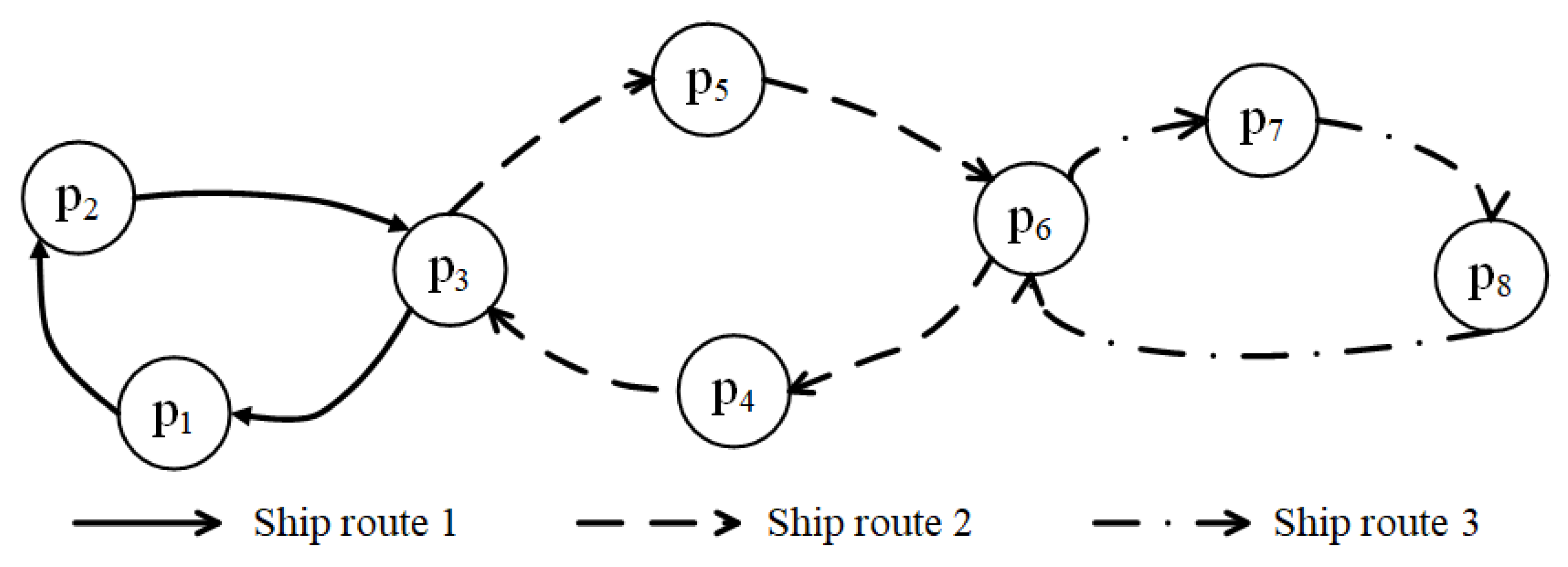
3. Problem Statement

In this section, we describe the studied problem. Especially, repacking operations are illustrated by five modes of transportation based on the proposition of Wang et al. [6], and the related costs are calculated by an illustrative example.

Consider a shipping network (P, G), where P is the set of ports and G is the set of legs between two ports. Let H be the set of transshipment ports, i.e., the intersection ports of different shipping routes, where $H\subseteq P$. Let R and S be the sets of shipping routes and cargo routes, respectively. Let $R_j$ be the port set of shipping route j and H be the set of transshipment ports in the container liner ship network. For example, in Figure 2, there are four shipping routes $R_1=\{p_1,p_2,p_3\},R_2=\{p_3,p_4,p_5,p_6\},R_3=\{p_6,p_7,p_8\}$. The transshipment ports are $H=\{p_3,p_6\}$.

Let $L_s$ and $K_s$ be the port set and the packing (and repacking) port set of cargo route $s\in S$, respectively. Clearly, $K_s\subseteq L_s$ for any $s\in S$. This signifies that there may be several repacking and unpacking operations for a cargo route s. For any $p,q\in K_s$ where port p precedes port q, let $\langle p,q\rangle$ be a subset of $K_s$ that contains all the packing ports from p to q in $K_s$. Consider a cargo route s: $p_2\to p_3\to p_5\to p_6\to p_7\to p_8$ in Figure 2. In this cargo route s, $L_s=\{p_2,p_3,p_5,p_6,p_7,p_8\}$, $K_s=\{p_2,p_3,p_6,p_8\}$ and $\langle p_3,p_8\rangle =\{p_3,p_6,p_8\}$. Let $(m,n)\in G$ be a leg from port m to port n where $m,n\in L_s$. For simplicity, we use $\{p,q\}\subseteq G$ to denote the leg set of $L_s$. If port p and port q are adjacent, then $\{p,q\}$ denotes one leg. In Figure 2, for example, $(m,n)\in \{p_4,p_8\}$ denotes that (m, n) is one leg of $p_4\to p_3$, $p_3\to p_5$, $p_5\to p_6$, $p_6\to p_7$ and $p_7\to p_8$. We use o and d to denote the origin port and the destination port, respectively.

In line with Wang et al. [6], the problem assumptions are summarized as follows:

(1)

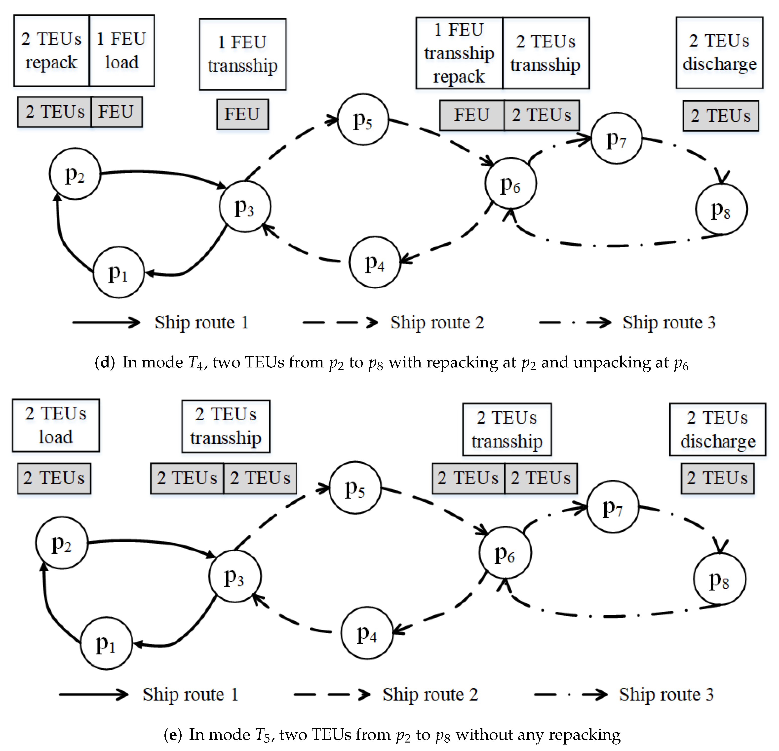
The repacking operations can only be executed at container yards. Therefore, before TEUs are repackaged into FEUs, containers need to be discharged from the liner ship, and then unload costs are incurred.

(2)

Each TEU and FEU are repacked at most once for a cargo route $s\in S$.

(3)

The uncertain demand of each cargo route is considered, and it is assumed to be not over the capacity of a cargo route.

(4)

Repacking operations can occur at transshipment ports, origin and destination ports.

(5)

The capacity of a shipping route is limited. That is, the numbers of transported TEUs and FEUs at each leg are less than or equal to the capacity of the shipping route. Note that we consider the capacity of the shipping route but not the capacity of the liner ship, because a shipping route has a group of liner ships to provide services.

To formulate the mathematical formulation, the repacking operations need to be discussed and summarized by five modes of transportation. Based on the proposition of Wang et al. [6], we can divide the repacking operations into five modes (see

Table 2. The enumeration of all five modes.

Modes	Origin Port	Transshipment Port	Destination Port
$T_1$	2TEUs→1FEU	None	1FEU→2TEUs
$T_2$	None	2TEUs→1FEU	1FEU→2TEUs
$T_3$	None	2TEUs→1FEU 1FEU→2TEUs	None
$T_4$	2TEUs→1FEU	1FEU→2TEUs	None
$T_5$	2TEUs	None	2TEUs

). The first column in Table 2 represents the number of modes denoted as $T_i$, $i=1,2,3,4,5$. The second, third and fourth columns indicate the different repacking operations at ports of origin, transshipment and destination, respectively. Let 2TEUs→1FEU denote the repacking from two TEUs into one FEU and let 1FEU→2TEUs denote the unpacking from one FEU into two TEUs.

To analyze the container handling costs of the five operating modes, we first introduce the following notations. Let ${\overline{c}}_p^T$, ${\tilde{c}}_p^T$ and ${\widehat{c}}_p^T$ be the loading, transshipment, and discharge costs of one TEU at a port p, respectively. The loading, transshipment, and discharge costs of one FEU at port p are denoted as ${\overline{c}}_p^F$, ${\tilde{c}}_p^F$, and ${\widehat{c}}_p^F$, respectively. To consider repacking operations, the repacking and unpacking costs of two TEUs and one FEU at port p are denoted as $c_p^T$ and $c_p^F$, respectively. $x_{sod}^{pq}$ denotes the number of TEUs that are repacked at port p ($p\in K_s$) and unpacked at port q ($q\in K_s$) while transshipping the containers, where $o,d$ are the origin and destination ports of cargo route s, respectively. ${\widehat{x}}_{sod}$ denotes the number of TEUs without repacking operations. Let $C_{T_1}$, $C_{T_2}$, $C_{T_3}$ and $C_{T_4}$ be the costs for loading, discharge, repacking and unpacking operations at the origin and destination ports, respectively.

The first mode, denoted as $T_1$, is the situation where two TEUs are repacked into one FEU at the origin port and later unpacked at the destination port. In line with Wang et al. [6], $C_{T_1}$ can be calculated as follows:

$$C_{T_1}=\frac{1}{2}·\sum _{s\in S}\left[\left(c_o^T+{\overline{c}}_o^F+{\widehat{c}}_d^F+c_d^F\right)·x_{sod}^{od}\right].$$

(1)

In the second mode $T_2$, two TEUs are loaded at the origin port, repacked at a transshipment port and unpacked at the destination port. $C_{T_2}$ can be calculated as follows:

$$C_{T_2}=\sum _{s\in S}\left({\overline{c}}_o^T+\frac{{\widehat{c}}_d^F}{2}+\frac{c_d^F}{2}\right)·\sum _{p\in K_s\setminus \{o,d\}}{x}_{sod}^{pd}.$$

(2)

In the third mode $T_3$, two TEUs are loaded at the origin port, repacked and unpacked at two respective transshipment ports, and finally discharged at the destination port. In line with Wang et al. [6], $C_{T_3}$ can be calculated as follows:

$$C_{T_3}=\sum _{s\in S}\left({\overline{c}}_o^T+\frac{{\widehat{c}}_d^F}{2}\right)·\sum _{p\in K_s\setminus \{o,d\}}\sum _{q\in K_s\setminus \{o,d\}}{x}_{sod}^{pq}.$$

(3)

The fourth mode $T_4$ describes the situation where two TEUs are repacked at the origin port and later unpacked into two TEUs at a transshipment port. $C_{T_4}$ can be calculated as follows:

$$C_{T_4}=\sum _{s\in S}\left(\frac{{\overline{c}}_o^F}{2}+\frac{c_o^T}{2}+{\widehat{c}}_d^T\right)·\sum _{q\in K_s\setminus \{o,d\}}{x}_{sod}^{oq}.$$

(4)

The fifth mode $T_5$ depicts that only the TEUs form is used at both the origin and destination ports without repacking or unpacking the whole way. $C_{T_5}$ can be calculated as follows:

$$C_{T_5}=\sum _{s\in S}\left[({\overline{c}}_o^T+{\widehat{c}}_d^T)·{\widehat{x}}_{sod}\right].$$

(5)

Figure 3 illustrates an example of transporting two TEUs from port $p_2$ to port $p_8$. In mode $T_1$, at the origin port $p_2$, two TEUs are repacked into one FEU, which is loaded on the liner ship. Then, the FEU is transshipped at ports $p_3$ and $p_6$ sequentially, and finally the FEU is discharged and unpacked at destination port $p_8$. Please see Figure 3a. In this situation, $C_{T_1}$ can be calculated as: $C_{T_1}=c_{p_2}^T+{\overline{c}}_{p_2}^F+{\widehat{c}}_{p_8}^F+c_{p_8}^F$. As shown in Figure 3b, in mode $T_2$, two TEUs are loaded at origin port $p_2$. At port $p_3$, the two TEUs are repacked into one FEU. Then, the FEU is transshipped at ports $p_3$ and $p_6$ sequentially, and finally, at destination port $p_8$, the FEU is discharged and unpacked into two TEUs. $C_{T_2}$ can be calculated as: $C_{T_2}=2{\overline{c}}_{p_2}^T+{\widehat{c}}_{p_8}^F+c_{p_8}^F$. As shown in Figure 3c, at origin port $p_2$, two TEUs are loaded. At port $p_3$, the two TEUs are repacked into one FEU and transported to port $p_6$. At port $p_6$, the FEU is discharged, unpacked into two TEUs, and reloaded on a liner ship. Finally, at destination port $p_8$, the two TEUs are discharged. $C_{T_3}$ can be calculated as: $C_{T_3}=2{\overline{c}}_{p_2}^T+2{\widehat{c}}_{p_8}^T$. In mode $T_4$, at the origin port $p_2$, two TEUs are repacked into one FEU, which is loaded on a liner ship. At port $p_6$, the FEU is discharged, unpacked into two TEUs, and reloaded on a liner ship. Finally, at destination port $p_8$, the two TEUs are discharged. Please see Figure 3d. $C_{T_4}$ can be calculated as: $C_{T_4}=c_{p_2}^T+{\overline{c}}_{p_2}^F+2{\widehat{c}}_{p_8}^F$. As shown in Figure 3e, in mode $T_5$, two TEUs are transported from port $p_2$ to port $p_8$ sequentially, and the repacking operations are not executed. $C_{T_5}$ can be calculated as follows: $C_{T_5}=2{\overline{c}}_{p_2}^T+2{\widehat{c}}_{p_8}^T$.

To analyze the handling cost of empty containers for loading, discharge, repacking and unpacking operations at the origin and destination ports, we first introduce the following notations. $z_{sod}^T$ denotes the number of empty TEUs from o to d in cargo route $s\in S$. $z_{sod}^F$ denotes the number of empty FEUs from o to d in cargo route $s\in S$. $C_E$ denotes the handling cost for loading, discharge, repacking and unpacking operations at the origin and destination ports. Since empty containers cannot be repacked, the handling cost of empty containers is similar to mode 5 ($T_5$), i.e., container transshipment without repacking operations. $C_E$ can be calculated as follows:

$$C_E=\sum _{s\in S}\left[({\overline{c}}_o^T+{\widehat{c}}_d^T)·z_{sod}^T+({\overline{c}}_o^F+{\widehat{c}}_d^F)·z_{sod}^F\right].$$

(6)

In the following section, we propose a distribution-free chance-constrained programming model to handle ambiguous laden and empty container demands, in which the costs of origin and destination ports and the numbers of transshipment containers of shipping routes are calculated according to the above five modes.

4. Mathematical Formulation

In this section, we first introduce some notations and apply moment-based uncertain sets to portray the ambiguous demands. Then, we construct a new distribution-free formulation with chance constraints.

4.1. Notations and Moment-Based Ambiguity Set

A moment-based ambiguity set is introduced to describe the uncertain laden container demand, and similarly, another two ambiguity sets are built to portray the empty TEU demand and empty FEU demand, respectively. For ease of modeling, we assume that shipment demands between different cargo routes are independent. Let $\mathsf{\Omega }$ and $\omega$ denote the set of laden container demand samples and the index of the set, respectively, and $\left|\mathsf{\Omega }\right|$ denotes the cardinality of set $\mathsf{\Omega }$. We use $\left|S\right|$ to denote the cardinality of set S. The historical laden container demand is assumed to be ${\left\{{\mathit{y}}^{\mathit{\omega }}\right\}}_{\omega =1}^{\left|\mathsf{\Omega }\right|}$ and ${\mathit{y}}^{\mathit{\omega }}={\{y_1^{\omega },y_2^{\omega },\dots ,y_{\left|S\right|}^{\omega }\}}^T$, where $y_s^{\omega }$ ($1\le s\le \left|S\right|$) is the laden container demand of cargo route s in scenario $\omega$. The mean vector $\mathit{\mu }$ and variance vector $\mathbf{\Sigma }$ of demand can be estimated as:

$$\mathit{\mu }=\frac{1}{\left|\mathsf{\Omega }\right|}·\sum _{\omega \in \mathsf{\Omega }}{\mathit{y}}^{\mathit{\omega }},\mathbf{\Sigma }=\frac{1}{\left|\mathsf{\Omega }\right|}·\sum _{\omega \in \mathsf{\Omega }}({\mathit{y}}^{\mathit{\omega }}-\mathit{\mu }){({\mathit{y}}^{\mathit{\omega }}-\mathit{\mu })}^{\top }.$$

(7)

Theoretically, $\mathit{\mu }$ and $\mathbf{\Sigma }$ converge to the true mean and covariance of demand as $\left|\mathsf{\Omega }\right|\to \infty$ [19]. Therefore, the set of all possible probability distributions of laden container demand, denoted by ${\Xi }_s({\mu }_s,{\Sigma }_s)$, of cargo route $s\in S$ can be described as:

$${\Xi }_s({\mu }_s,{\Sigma }_s)=\left\{{\mathbb{P}}_s:\begin{array}{c}{\mathbb{E}}_{{\mathbb{P}}_s}\left[y_s\right]={\mu }_s\hfill \\ {\mathbb{E}}_{{\mathbb{P}}_s}\left[{(y_s-{\mu }_s)}^2\right]={\Sigma }_s\hfill \end{array}\right\},$$

(8)

where ${\mathbb{P}}_s$ denotes a possible probability distribution of the laden container demand of cargo route s satisfying the given conditions, and $\mathbb{E}[·]$, with respect to ${\mathbb{P}}_s$, denotes the expected value of the expression in the brackets [19].

Similarly, let ${\mathsf{\Omega }}^T$ and $\omega$ denote the set of empty TEU container demand samples and the index of the set, respectively, and $\left|{\mathsf{\Omega }}^T\right|$ denotes the cardinality of set ${\mathsf{\Omega }}^T$. The historical empty TEU demand is assumed to be ${\left\{{\mathit{e}}^{\mathit{T}\mathit{\omega }}\right\}}_{\omega =1}^{\left|{\mathsf{\Omega }}^T\right|}$ and ${\mathit{e}}^{\mathit{T}\mathit{\omega }}={\{e_1^{T\omega },e_2^{T\omega },\dots ,e_{\left|S\right|}^{T\omega }\}}^{\top }$, where $e_s^{T\omega }$ ($1\le s\le \left|S\right|$) is the empty TEU container demand of cargo route s in scenario $\omega$. The mean vector ${\mathit{\mu }}^{\mathit{T}}$ and variance vector ${\mathbf{\Sigma }}^{\mathit{T}}$ of demand can be estimated as:

$${\mathit{\mu }}^T=\frac{1}{\left|{\mathsf{\Omega }}^T\right|}·\sum _{\omega \in {\mathsf{\Omega }}^T}{\mathit{e}}^{\mathit{T}\mathit{\omega }},{\mathbf{\Sigma }}^T=\frac{1}{\left|{\mathsf{\Omega }}^T\right|}·\sum _{\omega \in {\mathsf{\Omega }}^T}({\mathit{e}}^{\mathit{T}\mathit{\omega }}-{\mathit{\mu }}^T){({\mathit{e}}^{\mathit{T}\mathit{\omega }}-{\mathit{\mu }}^T)}^{\top }.$$

(9)

Similarly, the set of all possible probability distributions of empty TEU demand, denoted by ${\Xi }_s^T({\mu }_s^T,{\Sigma }_s^T)$, of cargo route $s\in S$ can be described as:

$${\Xi }_s^T({\mu }_s^T,{\Sigma }_s^T)=\left\{{\mathbb{P}}_s^T:\begin{array}{c}{\mathbb{E}}_{{\mathbb{P}}_s^T}\left[e_s^T\right]={\mu }_s^T\hfill \\ {\mathbb{E}}_{{\mathbb{P}}_s^T}\left[{(e_s^T-{\mu }_s^T)}^2\right]={\Sigma }_s^T\hfill \end{array}\right\},$$

(10)

where ${\mathbb{P}}_s^T$ denotes a possible probability distribution of the empty TEU container demand of cargo route s satisfying the given conditions.

Similarly, let ${\mathsf{\Omega }}^F$ and $\omega$ denote the set of empty FEU container demand samples and the index of the set, respectively, and let $\left|{\mathsf{\Omega }}^F\right|$ denote the cardinality of set ${\mathsf{\Omega }}^F$. The historical empty FEU container demand is assumed to be ${\left\{{\mathit{e}}^{\mathit{F}\mathit{\omega }}\right\}}_{\omega =1}^{\left|{\mathsf{\Omega }}^F\right|}$ and ${\mathit{e}}^{\mathit{F}\mathit{\omega }}={\{e_1^{F\omega },e_2^{F\omega },\dots ,e_{\left|S\right|}^{F\omega }\}}^{\top }$, where $e_s^{F\omega }$ ($1\le s\le \left|S\right|$) is the empty FEU container demand of cargo route s in scenario $\omega$. The mean vector ${\mathit{\mu }}^{\mathit{F}}$ and variance vector ${\mathbf{\Sigma }}^{\mathit{F}}$ of demand can be estimated as:

$${\mathit{\mu }}^F=\frac{1}{\left|{\mathsf{\Omega }}^F\right|}·\sum _{\omega \in {\mathsf{\Omega }}^F}{\mathit{e}}^{\mathit{F}\mathit{\omega }},{\mathbf{\Sigma }}^F=\frac{1}{\left|{\mathsf{\Omega }}^F\right|}·\sum _{\omega \in {\mathsf{\Omega }}^F}({\mathit{e}}^{\mathit{F}\mathit{\omega }}-{\mathit{\mu }}^F){({\mathit{e}}^{\mathit{F}\mathit{\omega }}-{\mathit{\mu }}^F)}^{\top }.$$

(11)

Similarly, the set of all possible probability distributions of empty FEU demand, denoted by ${\Xi }_s^F({\mu }_s^F,{\Sigma }_s^F)$, of cargo route $s\in S$ can be described as:

$${\Xi }_s^F({\mu }_s^F,{\Sigma }_s^F)=\left\{{\mathbb{P}}_s^F:\begin{array}{c}{\mathbb{E}}_{{\mathbb{P}}_s^F}\left[e_s^F\right]={\mu }_s^F\hfill \\ {\mathbb{E}}_{{\mathbb{P}}_s^F}\left[{(e_s^F-{\mu }_s^F)}^2\right]={\Sigma }_s^F\hfill \end{array}\right\},$$

(12)

where ${\mathbb{P}}_s^F$ denotes a possible probability distribution of the empty FEU container demand of cargo route s satisfying the given conditions.

4.2. Formulation

Additional problem parameters:

$V_j^T$:

the capacity of both empty and laden TEUs in shipping route $j\in R$;

$V_j^F$:

the capacity of both empty and laden FEUs in shipping route $j\in R$;

$y_s$:

the laden TEU demand of cargo route $s\in S$, random parameter;

$e_s^T$:

the empty TEU demand of cargo route $s\in S$, random parameter;

$e_s^F$:

the empty FEU demand of cargo route $s\in S$, random parameter;

${\alpha }_s$:

the maximum probability of failing to meet the demand of the laden TEUs in cargo route $s\in S$; Note that laden FEUs derived from repacking operations are finally unpacked to laden TEUs in cargo route s;

${\beta }_s$:

the maximum probability of failing to meet the demand of the empty TEUs in cargo route $s\in S$;

${\gamma }_s$:

the maximum probability of failing to meet the demand of the empty FEUs in cargo route $s\in S$.

Decision variables:

$x_{sod}^{pq}$:

the number of laden TEUs that are repacked at port p ($p\in K_s$) and unpacked at port q ($q\in K_s$) while transshipping the laden containers, where $o,d$ are the origin and destination ports of cargo route $s\in S$, respectively;

${\widehat{x}}_{sod}$:

the number of laden TEUs without repacking operations from o to d in cargo route $s\in S$;

$z_{sod}^T$:

the number of empty TEUs from o to d in cargo route $s\in S$;

$z_{sod}^F$:

the number of empty FEUs from o to d in cargo route $s\in S$;

$f_{jpq}^T$:

TEU flow of leg ($p,q$) of shipping route j, where $p,q\in R_j$;

$f_{jpq}^F$:

FEU flow of leg ($p,q$) of shipping route j, where $p,q\in R_j$;

$x_{spq}^T$:

TEU flow of leg ($p,q$) of cargo route s, where $p,q\in L_s$;

$x_{spq}^F$:

FEU flow of leg ($p,q$) of cargo route s, where $p,q\in L_s$;

$y_p^T$:

the quantity of laden and empty TEUs transshipped at port $p\in H$;

$y_p^F$:

the quantity of laden and empty FEUs transshipped at port $p\in H$;

$y_p^{TF}$:

the quantity of laden TEUs repacked into FEUs at port $p\in H$;

$y_p^{FT}$:

the quantity of laden FEUs unpacked into TEUs at port $p\in H$;

$C_{trans}$:

the transshipment cost of all ports;

$C_{pack}$:

the total packing cost incurred at all ports in the transshipment port set H;

$C_{load}$:

the cost for loading, discharge, repacking and unpacking operations at the origin and destination ports;

$C_E$:

the costs of both empty TEU and FEU containers for loading, discharge, repacking and unpacking operations at the origin and destination ports.

Formulation with chance constraints [${\mathit{ϝ}}_{\mathbf{1}}$]:

$$min{f}_1=C_{trans}+C_{pack}+C_{load}$$

(13)

Formula (13) is the objective function, i.e., minimizing the total cost that consists of transshipment cost, packing (repacking and unpacking) cost, and loading (loading and unloading) cost.

$$s.t.\left(1\right)\text{–}\left(6\right)$$

Equations (1)–(6) count the sum of loading, discharge, packing costs for all kinds of containers, respectively.

$$\begin{array}{c}\hfill C_{trans}=\sum _{p\in H}\left({\tilde{c}}_p^T·y_p^T+{\tilde{c}}_p^F·y_p^F\right)+\sum _{p\in H}\left[\left(\frac{{\tilde{c}}_p^T}{2}+\frac{{\tilde{c}}_p^F}{4}\right)·y_p^{TF}\right]+\sum _{p\in H}\left[\left(\frac{{\tilde{c}}_p^T}{2}+\frac{{\tilde{c}}_p^F}{4}\right)·y_p^{FT}\right]\end{array}$$

(14)

Equation (14) states the transshipment cost of all ports. The formula on the right-hand side of the equation contains three items. The first item ${\sum }_{p\in H}\left({\tilde{c}}_p^T·y_p^T+{\tilde{c}}_p^F·y_p^F\right)$ counts the transshipment cost of ports without any repacking or unpacking operations. The second item ${\sum }_{p\in H}\left(\frac{{\tilde{c}}_p^T}{2}+\frac{{\tilde{c}}_p^F}{4}\right)·y_p^{TF}$ calculates the transportation cost with repacking. The last item is the unpacking cost of ports.

$$C_{pack}=\sum _{p\in H}\left(c_p^T·\frac{y_p^{TF}}{2}+c_p^F·y_p^{FT}\right)$$

(15)

$C_{pack}$ denotes the total packing cost incurred at all ports in the transshipment port set H. Note that the packing cost incurred at origin and destination ports is not included.

$$C_{load}=C_{T_1}+C_{T_2}+C_{T_3}+C_{T_4}+C_{T_5}+C_E$$

(16)

$C_{load}$ is the cost for loading, discharge, repacking and unpacking operations at the origin and destination ports. Equation (16) shows that the cost consists of six terms, corresponding to five transportation modes, i.e., $T_1,T_2,T_3,T_4,T_5$, and E, respectively, which are calculated as follows.

$$\begin{array}{c}\hfill y_m^T=\sum _{s\in S}\sum _{p\in \langle m,d\rangle \setminus \{m,d\}}\sum _{q\in \langle o,m\rangle \setminus \{o,m\}}{x}_{sod}^{pq}+\sum _{s\in S}({\widehat{x}}_{sod}+z_{sod}^T)m\in H\end{array}$$

(17)

$$y_m^F=\sum _{s\in S}\sum _{p\in \langle o,m\rangle \setminus \left\{m\right\}}\sum _{q\in \langle m,d\rangle \setminus \left\{m\right\}}{x}_{sod}^{pq}+\sum _{s\in S}{z}_{sod}^{F}m\in H$$

(18)

Equations (17) and (18) calculate the numbers of TEUs and FEUs transshipped at port $m\in H$.

$$y_m^{TF}=\sum _{s\in S}\sum _{q\in \langle m,d\rangle \setminus \left\{m\right\}}{x}_{sod}^{mq}m\in H$$

(19)

$$y_m^{FT}=\frac{1}{2}·\sum _{s\in S}\sum _{p\in \langle o,m\rangle \setminus \left\{m\right\}}{x}_{sod}^{pm}m\in H$$

(20)

Equations (19) and (20) give the number of TEUs repacked into FEUs and FEUs unpacked into TEUs at port $m\in H$.

$$\begin{array}{c}\hfill x_{smv}^T=\sum _{q\in \langle o,m\rangle \setminus \left\{o\right\}}\sum _{p\in \langle o,q\rangle \setminus \left\{q\right\}}{x}_{sod}^{pq}+\sum _{p\in \langle v,d\rangle \setminus \left\{d\right\}}\sum _{q\in \langle p,d\rangle \setminus \left\{p\right\}}{x}_{sod}^{pq}+{\widehat{x}}_{sod}+z_{sod}^{T}s\in S,(m,v)\in \{o,d\}\end{array}$$

(21)

$$x_{smv}^F=\frac{1}{2}·\sum _{p\in \langle o,m\rangle }\sum _{q\in \langle v,d\rangle }{x}_{sod}^{pq}+z_{sod}^{F}s\in S,(m,v)\in \{o,d\}$$

(22)

Equations (21) and (22) state the TEU and FEU flows of cargo route legs. The container flow of each leg is composed of the containers with repacking operations and the ones transported by TEU.

$$f_{jpq}^T=\sum _{s\in S}{x}_{spq}^{T}j\in R,p,q\in R_j,\{p,q\}\in G$$

(23)

$$f_{jpq}^F=\sum _{s\in S}{x}_{spq}^{F}j\in R,p,q\in R_j,\{p,q\}\in G$$

(24)

Different cargo routes may pass the same leg in one shipping route. Equations (23) and (24) calculate the TEU and FEU flows for each leg, respectively.

$$f_{jpq}^T\le V_j^{T}j\in R,p,q\in R_j,\{p,q\}\in G$$

(25)

$$f_{jpq}^F\le V_j^{F}j\in R,p,q\in R_j,\{p,q\}\in G$$

(26)

Inequalities (25) and (26) are shipping route capacity constraints.

$$\begin{array}{c}\hfill \underset{{\mathbb{P}}_s\in {\Xi }_s}{inf}P{r}_{{\mathbb{P}}_s}\left\{\sum _{p\in K_s\setminus \{o,d\}}\sum _{q\in K_s\setminus \{o,d\}}{x}_{sod}^{pq}+{\widehat{x}}_{sod}\ge y_s\right\}\ge 1-{\alpha }_{s}s\in S\end{array}$$

(27)

$$\begin{array}{c}\hfill \underset{{\mathbb{P}}_s^T\in {\Xi }_s^T}{inf}P{r}_{{\mathbb{P}}_s^T}\left\{z_{sod}^T\ge e_s^T\right\}\ge 1-{\beta }_{s}s\in S\end{array}$$

(28)

$$\begin{array}{c}\hfill \underset{{\mathbb{P}}_s^F\in {\Xi }_s^F}{inf}P{r}_{{\mathbb{P}}_s^F}\left\{z_{sod}^F\ge e_s^F\right\}\ge 1-{\gamma }_{s}s\in S\end{array}$$

(29)

Constraints (27)–(29) are chance constraints in which the demands of laden TEU, empty TEU and empty FEU in cargo route $s\in S$ are met with a probability of at least $1-{\alpha }_s$, $1-{\beta }_s$ and $1-{\gamma }_s$, respectively. $P{r}_{{\mathbb{P}}_s}\{·\}$, $P{r}_{{\mathbb{P}}_s^T}\{·\}$, and $P{r}_{{\mathbb{P}}_s^F}\{·\}$ denote the probabilities with respect to ${\mathbb{P}}_s$, ${\mathbb{P}}_s^T$, and ${\mathbb{P}}_s^F$, respectively.

5. Distribution-Free Approximation Approaches

In this section, we apply four distribution-free approaches, i.e., SAA, eSAA, AMI, and MI-SOCP, to approximate the chance constraints in this problem.

5.1. Sample Average Approximation (SAA)

SAA is employed to solve large-scale stochastic optimization problems via Monte Carlo simulation, which is widely applied in different fields [36]. It applies historical scenarios to portray the uncertainty of the problem when the distribution is unknown [39]. In other words, SAA is used to transform the stochastic programming problem into a sample average estimation through many scenarios. To approximate model ${\mathit{ϝ}}_{\mathbf{1}}$, we generate scenarios with respect to three distributions, normal, uniform and mixed (normal and uniform) of the uncertain demand $y_s\left(\omega \right)$, $e_s^T\left(\omega \right)$, and $e_s^F\left(\omega \right)$, respectively.

Formulation with distribution [${\mathit{ϝ}}_{\mathbf{2}}$]:

New parameters:

$\varsigma$:

a sufficiently large positive number;

$y_s\left(\omega \right)$:

the laden TEU demand of cargo route s in scenario $\omega$;

$e_s^T\left(\omega \right)$:

the empty TEU demand of cargo route s in scenario $\omega$;

$e_s^F\left(\omega \right)$:

the empty FEU demand of cargo route s in scenario $\omega$;

New decision variables:

${\Theta }_s\left(\omega \right)$:

binary variable, equal to 0 if the number of transshipment laden TEU containers meets the demand of cargo route s in scenario $\omega$, 1 otherwise;

${\mathsf{\Phi }}_s\left(\omega \right)$:

binary variable, equal to 0 if the number of empty TEU containers meets the demand of cargo route s in scenario $\omega$, 1 otherwise;

${\mathsf{\Gamma }}_s\left(\omega \right)$:

binary variable, equal to 0 if the number of empty FEU containers meets the demand of cargo route s in scenario $\omega$, 1 otherwise.

$$min{f}_1$$

$$s.t.\left(14\right)\text{–}\left(26\right)$$

$$\begin{array}{c}\hfill \sum _{p\in K_s\setminus \{o,d\}}\sum _{q\in K_s\setminus \{o,d\}}{x}_{sod}^{pq}+{\widehat{x}}_{sod}\ge y_s\left(\omega \right)·(1-{\Theta }_s\left(\omega \right))s\in S,\omega \in \mathsf{\Omega }\end{array}$$

(30)

$$\sum _{\omega \in \mathsf{\Omega }}{\Theta }_s\left(\omega \right)\le \left|\mathsf{\Omega }\right|·{\alpha }_{s}s\in S$$

(31)

$$\begin{array}{c}\hfill z_{sod}^T\ge e_s^T\left(\omega \right)·(1-{\mathsf{\Phi }}_s\left(\omega \right))s\in S,\omega \in {\mathsf{\Omega }}^T\end{array}$$

(32)

$$\sum _{\omega \in {\mathsf{\Omega }}^T}{\mathsf{\Phi }}_s\left(\omega \right)\le \left|{\mathsf{\Omega }}^T\right|·{\beta }_{s}s\in S$$

(33)

$$\begin{array}{c}\hfill z_{sod}^F\ge e_s^F\left(\omega \right)·(1-{\mathsf{\Gamma }}_s\left(\omega \right))s\in S,\omega \in {\mathsf{\Omega }}^F\end{array}$$

(34)

$$\sum _{\omega \in {\mathsf{\Omega }}^F}{\mathsf{\Gamma }}_s\left(\omega \right)\le \left|{\mathsf{\Omega }}^F\right|·{\gamma }_{s}s\in S$$

(35)

Constraints (27)–(29) are replaced by constraints (30)–(35) in the model ${\mathit{ϝ}}_{\mathbf{2}}$. Constraint (30) states that laden TEU containers are not less than the demand when ${\Theta }_s\left(\omega \right)$ equals 0. Constraint (31) ensures that the laden TEU containers can meet the demand of cargo route s with a probability of no less than $1-{\alpha }_s$. Constraint (32) states that empty TEU containers are not less than the demand when ${\mathsf{\Phi }}_s\left(\omega \right)$ equals 0. Constraint (33) ensures that the empty TEU containers can meet the demand of cargo route s with a probability no less than $1-{\beta }_s$. Constraint (34) states that empty FEU containers are not less than the demand when ${\mathsf{\Gamma }}_s\left(\omega \right)$ equals 0. Constraint (35) ensures that the empty FEU containers can meet the demand of cargo route s with a probability no less than $1-{\gamma }_s$.

5.2. Enhanced Sample Average Approximation (eSAA)

SAA performs well under a large number of samples, but inappropriate samples may lead to low-quality solutions with a high computational burden [40]. Therefore, in this work, we utilize the clustering (K-means and K-means++) technique to update both sample sizes and sample qualities dynamically.

K-means clustering is a popular unsupervised algorithm proposed by Lloyd [41]. It works in two phases. In the first phase, initial cluster centers are selected randomly, and each data point is assigned to one of the clusters by distance. In the second phase, the core position of each cluster is updated and data points are reassigned accordingly. The second phase is repeated until the convergence requirement is satisfied. The SAA with K-means cluster algorithm is in Algorithm 1, which is called eSAA with K-means.

Algorithm 1: SAA with K-means clustering (eSAA with K-means)

Step 1: Set parameters: $N\leftarrow$ the number of scenarios; $K\leftarrow$ number of clusters; $C_k\leftarrow$ set of points that belongs to cluster k, where k = 1, 2, 3, …, K. Step 2: Generate N scenarios: ${\mathit{x}}_{\mathit{n}}$, where n = 1, 2, 3, …, N. Step 3: Randomly select K initial cluster centers recorded as ${\mathit{y}}_{\mathit{k}}$ from ${\mathit{x}}_{\mathit{n}}$, where n = 1, 2, 3, …, N, k = 1, 2, 3, …, K, $N\gg K$. Step 4: Attribute the nearest cluster to each data point: $C_k=\{i:d({\mathit{x}}_{\mathit{i}},{\mathit{y}}_{\mathit{k}})\le d({\mathit{x}}_{\mathit{i}},{\mathit{y}}_{\mathit{j}}),j=1,2,3,\dots ,K,j\ne k,i=1,2,3,\dots ,N\}$, where k = 1, 2, 3, …, K. Step 5: Fix the position of each cluster by calculating the mean of all points belonging to that cluster: ${\mathit{y}}_{\mathit{k}}=\frac{1}{\left|C_k\right|}{\sum }_{i\in C_k}{\mathit{x}}_{\mathit{i}}$. Step 6: Repeat Step 4 and Step 5 until convergence. Step 7: Randomly select one sample of each cluster as input. Step 8: Solve the model ${\mathit{ϝ}}_{\mathbf{2}}$ by CPLEX.

Arthur and Vassilvitskii [42] developed K-means++ based on K-means. The difference between K-means++ and K-means is in the phase of initializing cluster centers. In the K-means++ algorithm, cluster centers are selected with some probability, which is ensured by the distances between data points and the core of cluster centers. The detail of SAA with K-means++ is represented in Algorithm 2, which is called eSAA with K-means++.

Algorithm 2: SAA with K-means++ clustering (eSAA with K-means++)

Step 1: The same as Step 1 of Algorithm 1. Step 2: The same as Step 2 of Algorithm 1. Step 3: Randomly select one cluster center, recorded as ${\mathit{y}}_{\mathbf{1}}$, from ${\mathit{x}}_{\mathit{n}}$, where n = 1, 2, 3, …, N; set $m=2$; Step 4: Calculate the core of m cluster center(s) recorded as $\mathit{z}$: $\mathit{z}=\frac{1}{m-1}{\sum }_{i=1}^{m-1}{\mathit{y}}_{\mathit{i}}$ Step 5: Select one sample ${\mathit{x}}_{\mathit{i}}$ ($i=1,2,3,\dots ,N$) apart from ${\mathit{x}}_{\mathit{n}}$ as cluster center recorded as $y_m$ with probability: $\frac{d(\mathit{z},{\mathit{x}}_{\mathit{n}})}{{\sum }_{n=1}^{N}d(\mathit{z},{\mathit{x}}_{\mathit{n}})}$. Step 6: Set $m=m+1$, repeat Step 4 and Step 5 when $m\le K$. Step 7: The same as Step 4 of Algorithm 1. Step 8: The same as Step 5 of Algorithm 1. Step 9: Repeat Step 7 and Step 8 until convergence. Step 10: The same as Step 7 of Algorithm 1. Step 11: The same as Step 8 of Algorithm 1.

5.3. An Approximation Based on Markov’s Inequality (AMI)

Both SAA and eSAA generate plenty of scenarios to simulate the stochastic problem approximatively. Theoretically, the larger the number of scenarios, the better the solutions. However, it is impractical to solve a large number of scenarios due to consuming an unreasonable running time. Therefore, it is necessary to develop more practical approaches to solve the stochastic problem.

Below, we introduce an approximate method, which only requires empirical mean and variance. The method is mainly derived from Markov’s inequality, i.e., Equation (36). A proof of transformation of chance constraints (27)–(29) is given below in detail based on the paper [13].

$$Pr\{\left|X\right|\ge a\}\le \frac{\mathbb{E}\left(X\right)}{a}$$

(36)

Theorem 1

([13]). As for ${\nu }_s$, ${\nu }_s^T$ and ${\nu }_s^F$ given by functions $g_s(·)$, $g_s^T(·)$, and $g_s^F(·)$, the chance constraints (27)–(29) are equivalent to the following constraints (37)–(45).

$$\sum _{p\in K_s\setminus \{o,d\}}\sum _{q\in K_s\setminus \{o,d\}}{x}_{sod}^{pq}+{\widehat{x}}_{sod}\ge {\mu }_s+{\nu }_{s}s\in S$$

(37)

$$\begin{array}{c}\hfill g_s\left({\nu }_s\right)\equiv \underset{\lambda >0}{min}\left(e^{\frac{-\lambda {\nu }_s}{{\mu }_s}}\left(1+\frac{{\Sigma }_s}{{\mu }_s^2{\kappa }_s^2}(e^{\lambda {\kappa }_s}-\lambda {\kappa }_s-1)\right)-{\alpha }_s\right)s\in S\end{array}$$

(38)

$$g_s\left({\nu }_s\right)=0s\in S$$

(39)

$$z_{sod}^T\ge {\mu }_s^T+{\nu }_s^{T}s\in S$$

(40)

$$\begin{array}{c}\hfill g_s^T\left({\nu }_s^T\right)\equiv \underset{\lambda >0}{min}\left(e^{\frac{-\lambda {\nu }_s^T}{{\mu }_s^T}}\left(1+\frac{{\Sigma }_s^T}{{\left({\mu }_s^T\right)}^2{\left({\kappa }_s^T\right)}^2}(e^{\lambda {\kappa }_s^T}-\lambda {\kappa }_s^T-1)\right)-{\beta }_s\right)s\in S\end{array}$$

(41)

$$g_s^T\left({\nu }_s^T\right)=0s\in S$$

(42)

$$z_{sod}^F\ge {\mu }_s^F+{\nu }_s^{F}s\in S$$

(43)

$$\begin{array}{c}\hfill g_s^F\left({\nu }_s^F\right)\equiv \underset{\lambda >0}{min}\left(e^{\frac{-\lambda {\nu }_s^F}{{\mu }_s^F}}\left(1+\frac{{\Sigma }_s^F}{{\left({\mu }_s^F\right)}^2{\left({\kappa }_s^F\right)}^2}(e^{\lambda {\kappa }_s^F}-\lambda {\kappa }_s^F-1)\right)-{\gamma }_s\right)s\in S\end{array}$$

(44)

$$g_s^F\left({\nu }_s^F\right)=0s\in S$$

(45)

where ${\Sigma }_s$, ${\Sigma }_s^T$, and ${\Sigma }_s^F$ are the empirical means of $y_s$, $e_s^T$, and $e_s^F$, respectively; ${\mu }_s$, ${\mu }_s^T$, and ${\mu }_s^F$ are the empirical variances of $y_s$, $e_s^T$, and $e_s^F$, respectively; λ is a positive number.

Before proving the above theorem related to constraints (37)–(39), we introduced two lemmas. ${\xi }_s$ is a random variable to model the deviation from the mean demand of cargo route s.

Lemma 1

([13]). Given $\lambda >0$, the following inequality holds:

$$\mathbb{E}\left[e^{\lambda {\xi }_s}\right]\le 1+\frac{\mathbb{E}\left[{\left({\xi }_s\right)}^2\right]}{{\left({\kappa }_s\right)}^2}(e^{\lambda {\kappa }_s}-\lambda {\kappa }_s-1)$$

(46)

The proof of Lemma 1 follows Lemma 2 in the work [13], and we omit the details here.

Lemma 2

([13]).

$$\mathbb{E}\left[{\xi }_s^2\right]·{\mu }_s^2={\Sigma }_s$$

(47)

Proof. 

Since

$${\Sigma }_s=\mathbb{E}\left[{(y_s-{\mu }_s)}^2\right]$$

and $y_s={\mu }_s(1+{\xi }_s)$, we have ${\Sigma }_s=\mathbb{E}\left[{\mu }_s^2{\xi }_s^2\right]$. The lemma follows, and the proof is completed. □

Now, we make the proof of Theorem 1.

Proof. 

First,

$$\begin{array}{c}\hfill Pr\left\{\sum _{p\in K_s\setminus \{o,d\}}\sum _{q\in K_s\setminus \{o,d\}}{x}_{sod}^{pq}+{\widehat{x}}_{sod}\ge y_s\right\}\end{array}.$$

As $y_s={\mu }_s(1+{\xi }_s)$, the above formula is equivalent to

$$Pr\left\{\sum _{p\in K_s\setminus \{o,d\}}\sum _{q\in K_s\setminus \{o,d\}}{x}_{sod}^{pq}+{\widehat{x}}_{sod}\ge {\mu }_s(1+{\xi }_s)\right\}.$$

When inequality ${\mu }_s+{\nu }_s\ge {\mu }_s(1+{\xi }_s)$ and Constraint (37) are established, the inequality in the brace above holds. The subsequent derivation process is as follows.

$$\begin{array}{c}\hfill Pr\left\{{\mu }_s+{\nu }_s\ge {\mu }_s(1+{\xi }_s)\right\}=Pr\left\{{\mu }_s{\xi }_s\le {\nu }_s\right\}=Pr\left\{\lambda {\xi }_s\le \frac{\lambda {\nu }_s}{{\mu }_s}\right\}=Pr\left\{e^{\lambda {\xi }_s}\le e^{\frac{\lambda {\nu }_s}{{\mu }_s}}\right\}\end{array}$$

Based on Markov’s Inequality (36),

$$Pr\left\{e^{\lambda {\xi }_s}\le e^{\frac{\lambda {\nu }_s}{{\mu }_s}}\right\}\le \mathbb{E}\left[e^{\lambda {\xi }_s}\right]·e^{\frac{-\lambda {\nu }_s}{{\mu }_s}}.$$

Substituting Inequality (46) and Equation (47) into the above inequality, we have

$$Pr\left\{e^{\lambda {\xi }_s}\le e^{\frac{\lambda {\nu }_s}{{\mu }_s}}\right\}\le e^{\frac{-\lambda {\nu }_s}{{\mu }_s}}·\left(1+\frac{{\Sigma }_s}{{\mu }_s^2{\kappa }_s^2}(e^{\lambda {\kappa }_s}-\lambda {\kappa }_s-1)\right).$$

Therefore, with similar analysis, we can show that Constraints (27)–(29) are equivalent to Constraints (37)–(45). □

Markov formulation [${\mathit{ϝ}}_{\mathbf{3}}$]:

$$min{f}_1$$

$$s.t.\left(14\right)\text{–}\left(26\right),\left(37\right)\text{–}\left(45\right)$$

5.4. Mixed Integer Second-Order Cone Program (MI-SOCP)

Alternatively, we adopt an approximation approach without scenarios for Constraints (27)–(29), which are called a mixed-integer second-order cone program. Based on Proposition 1 in Wagner [43], three ambiguity sets, i.e., ${\mathcal{D}}_s^{\mathcal{C}}$, ${\mathcal{D}}_s^{\mathcal{T}}$ and ${\mathcal{D}}_s^{\mathcal{F}}$, are defined as follows, in which ${\mu }_s^0$, ${\mu }_s^{T0}$ and ${\mu }_s^{F0}$ are true means of $y_s$, $e_s^T$ and $e_s^F$, respectively; ${\Sigma }_s^0$, ${\Sigma }_s^{T0}$, and ${\Sigma }_s^{F0}$ are true variances of $y_s$, $e_s^T$ and $e_s^F$, respectively.

$${\mathcal{D}}_s^{\mathcal{C}}({\Xi }_s,{\mu }_s^0,{\Sigma }_s^0)=\left\{{\mathbb{P}}_s:\begin{array}{c}{\displaystyle \sum _{\omega =1}^{\infty }}P{r}_{{\mathbb{P}}_s}\left(y_s\left(\omega \right)\right)=1\hfill \\ {\mathbb{E}}_{{\mathbb{P}}_s}\left[y_s\right]={\mu }_s^0\hfill \\ {\mathbb{E}}_{{\mathbb{P}}_s}\left[{(y_s-{\mu }_s^0)}^2\right]={\Sigma }_s^0\hfill \end{array}\right\}$$

$${\mathcal{D}}_s^{\mathcal{T}}({\Xi }_s^T,{\mu }_s^{T0},{\Sigma }_s^{T0})=\left\{{\mathbb{P}}_s^T:\begin{array}{c}{\displaystyle \sum _{\omega =1}^{\infty }}P{r}_{{\mathbb{P}}_s^T}\left(e_s^T\left(\omega \right)\right)=1\hfill \\ {\mathbb{E}}_{{\mathbb{P}}_s^T}\left[e_s^T\right]={\mu }_s^{T0}\hfill \\ {\mathbb{E}}_{{\mathbb{P}}_s^T}\left[{(e_s^T-{\mu }_s^{T0})}^2\right]={\Sigma }_s^{T0}\hfill \end{array}\right\}$$

$${\mathcal{D}}_s^{\mathcal{F}}({\Xi }_s^F,{\mu }_s^{F0},{\Sigma }_s^{F0})=\left\{{\mathbb{P}}_s^F:\begin{array}{c}{\displaystyle \sum _{\omega =1}^{\infty }}P{r}_{{\mathbb{P}}_s^T}\left(e_s^F\left(\omega \right)\right)=1\hfill \\ {\mathbb{E}}_{{\mathbb{P}}_s^F}\left[e_s^F\right]={\mu }_s^{F0}\hfill \\ {\mathbb{E}}_{{\mathbb{P}}_s^F}\left[{(e_s^F-{\mu }_s^{F0})}^2\right]={\Sigma }_s^{F0}\hfill \end{array}\right\}$$

According to Proposition 1 in Wagner [43], Constraint (27) can be replaced by Constraint (48) with a given risk ${\alpha }_s$.

$$\begin{array}{c}\hfill \sqrt{\frac{{\alpha }_s}{1-{\alpha }_s}}·\left(\sum _{p\in K_s\setminus \{o,d\}}\sum _{q\in K_s\setminus \{o,d\}}{x}_{sod}^{pq}+{\widehat{x}}_{sod}-{\mu }_s^0\right)\ge \sqrt{{\Sigma }_s^0}s\in S\end{array}.$$

(48)

Similarly, Constraints (28) and (29) can be replaced by Constraints (49) and (50).

$$\begin{array}{c}\hfill \sqrt{\frac{{\beta }_s}{1-{\beta }_s}}·\left(z_{sod}^T-{\mu }_s^{T0}\right)\ge \sqrt{{\Sigma }_s^{T0}}s\in S\end{array}.$$

(49)

$$\begin{array}{c}\hfill \sqrt{\frac{{\gamma }_s}{1-{\gamma }_s}}·\left(z_{sod}^F-{\mu }_s^{F0}\right)\ge \sqrt{{\Sigma }_s^{F0}}s\in S\end{array}.$$

(50)

The values of ${\mu }_s^0$, ${\mu }_s^{T0}$, ${\mu }_s^{F0}$, ${\Sigma }_s^0$, ${\Sigma }_s^{T0}$ and ${\Sigma }_s^{F0}$ are usually unknown in reality, but the empirical mean and variance are accessible by historical data. According to Theorem 2 in Zhang et al. [21], Constraint (48) is equivalent to Constraint (51) under risk parameter ${\alpha }_s$. Scalars ${\phi }_1$ and ${\phi }_2$ are related to the moment-based ambiguity set ${\mathcal{D}}_s^{\mathcal{M}}$ [19], which is used to characterize possible probability distribution ${\mathbb{P}}_s$ for each cargo route $s\in S$.

$${\mathcal{D}}_s^{\mathcal{M}}({\Xi }_s,{\mu }_s,{\Sigma }_s,{\gamma }_1,{\gamma }_2)=\left\{{\mathbb{P}}_s:\begin{array}{c}{\displaystyle \sum _{\omega =1}^{\infty }}P{r}_{{\mathbb{P}}_s}\left(y_s\left(\omega \right)\right)=1\hfill \\ {({\mathbb{E}}_{{\mathbb{P}}_s}\left[y_s\right]-{\mu }_s)}^2\le {\phi }_1{\Sigma }_s\hfill \\ {\mathbb{E}}_{{\mathbb{P}}_s}{[y_s-{\mu }_s]}^2\le {\phi }_2{\Sigma }_s\hfill \end{array}\right\}$$

where ${\phi }_1$ and ${\phi }_2$, with ${\phi }_2>{\phi }_1\ge 0$, are scalars to adjust the size of ${\mathcal{D}}_s^{\mathcal{M}}$. Moreover, the values of ${\phi }_1$ and ${\phi }_2$ affect the performance of model ${\mathit{ϝ}}_{\mathbf{4}}$.

$$\sqrt{\frac{1}{1-{\tau }_1-{\tau }_2}}·\left(1+\sqrt{\frac{{\alpha }_s·{\tau }_2}{1-{\alpha }_s}}\right)·\sqrt{{\Sigma }_s}\le \sqrt{\frac{{\alpha }_s}{1-{\alpha }_s}}·\left(\sum _{p\in K_s\setminus \{o,d\}}\sum _{q\in K_s\setminus \{o,d\}}{x}_{sod}^{pq}+{\widehat{x}}_{sod}-{\mu }_s\right)s\in S$$

(51)

where ${\tau }_1$, ${\tau }_2$ and ${\phi }_1$, ${\phi }_2$ have the following relations.

$${\tau }_1=\frac{{\phi }_2-2{\phi }_1-1}{{\phi }_2-{\phi }_1}.$$

(52)

$${\tau }_2=\frac{{\phi }_1}{{\phi }_2-{\phi }_1}.$$

(53)

Similarly, Constraint (49) is equivalent to Constraint (54) under risk parameter ${\beta }_s$. Scalars ${\phi }_1^T$ and ${\phi }_2^T$ are related to moment-based ambiguity set ${\mathcal{D}}_s^{T\mathcal{M}}$ [19], which is used to characterize possible probability distribution ${\mathbb{P}}_s^T$ for each cargo route $s\in S$.

$${\mathcal{D}}_s^{T\mathcal{M}}({\Xi }_s^T,{\mu }_s^T,{\Sigma }_s^T,{\gamma }_1^T,{\gamma }_2^T)=\left\{{\mathbb{P}}_s^T:\begin{array}{c}{\displaystyle \sum _{\omega =1}^{\infty }}P{r}_{{\mathbb{P}}_s^T}\left(e_s^T\left(\omega \right)\right)=1\hfill \\ {({\mathbb{E}}_{{\mathbb{P}}_s^T}\left[e_s^T\right]-{\mu }_s^T)}^2\le {\phi }_1^T{\Sigma }_s^T\hfill \\ {\mathbb{E}}_{{\mathbb{P}}_s^T}{[e_s^T-{\mu }_s^T]}^2\le {\phi }_2^T{\Sigma }_s^T\hfill \end{array}\right\}$$

where ${\phi }_1^T$ and ${\phi }_2^T$, with ${\phi }_2^T>{\phi }_1^T\ge 0$, are scalars to adjust the size of ${\mathcal{D}}_s^{T\mathcal{M}}$.

$$\sqrt{\frac{1}{1-{\tau }_1^T-{\tau }_2^T}}·\left(1+\sqrt{\frac{{\beta }_s·{\tau }_2^T}{1-{\beta }_s}}\right)·\sqrt{{\Sigma }_s^T}\le \sqrt{\frac{{\beta }_s}{1-{\beta }_s}}·\left(z_{sod}^T-{\mu }_s^T\right)s\in S,$$

(54)

where ${\tau }_1^T$, ${\tau }_2^T$ and ${\phi }_1^T$, ${\phi }_2^T$ have the following relations.

$${\tau }_1^T=\frac{{\phi }_2^T-2{\phi }_1^T-1}{{\phi }_2^T-{\phi }_1^T}.$$

(55)

$${\tau }_2^T=\frac{{\phi }_1^T}{{\phi }_2^T-{\phi }_1^T}.$$

(56)

Similarly, Constraint (50) is equivalent to Constraint (57) under risk parameter ${\gamma }_s$. Scalars ${\phi }_1^F$ and ${\phi }_2^F$ are related to moment-based ambiguity set ${\mathcal{D}}_s^{F\mathcal{M}}$ [19], which is used to characterize possible probability distribution ${\mathbb{P}}_s^F$ for each cargo route $s\in S$.

$${\mathcal{D}}_s^{F\mathcal{M}}({\Xi }_s^F,{\mu }_s^F,{\Sigma }_s^F,{\gamma }_1^F,{\gamma }_2^F)=\left\{{\mathbb{P}}_s^F:\begin{array}{c}{\displaystyle \sum _{\omega =1}^{\infty }}P{r}_{{\mathbb{P}}_s^F}\left(e_s^F\left(\omega \right)\right)=1\hfill \\ {({\mathbb{E}}_{{\mathbb{P}}_s^F}\left[e_s^F\right]-{\mu }_s^F)}^2\le {\phi }_1^F{\Sigma }_s^F\hfill \\ {\mathbb{E}}_{{\mathbb{P}}_s^F}{[e_s^F-{\mu }_s^F]}^2\le {\phi }_2^F{\Sigma }_s^F\hfill \end{array}\right\}$$

where ${\phi }_1^F$ and ${\phi }_2^F$, with ${\phi }_2^F>{\phi }_1^F\ge 0$, are scalars to adjust the size of ${\mathcal{D}}_s^{F\mathcal{M}}$.

$$\sqrt{\frac{1}{1-{\tau }_1^F-{\tau }_2^F}}·\left(1+\sqrt{\frac{{\gamma }_s·{\tau }_2^F}{1-{\gamma }_s}}\right)·\sqrt{{\Sigma }_s^F}\le \sqrt{\frac{{\gamma }_s}{1-{\gamma }_s}}·\left(z_{sod}^F-{\mu }_s^F\right)s\in S,$$

(57)

where ${\tau }_1^F$, ${\tau }_2^F$ and ${\phi }_1^F$, ${\phi }_2^F$ have the following relations.

$${\tau }_1^F=\frac{{\phi }_2^F-2{\phi }_1^F-1}{{\phi }_2^F-{\phi }_1^F}.$$

(58)

$${\tau }_2^F=\frac{{\phi }_1^F}{{\phi }_2^F-{\phi }_1^F}.$$

(59)

MI-SOCP formulation [${\mathit{ϝ}}_{\mathbf{4}}$]:

$$min{f}_1$$

$$s.t.\left(14\right)\text{–}\left(26\right),\left(51\right)\text{–}\left(59\right)$$

6. Computational Experiments

In this section, we first make a sensitivity analysis of the numbers of samples and scenarios in SAA and two eSAA versions (i.e., eSAA with K-means and eSAA with K-means++), and compare the performances of SAA and two eSAAs. Then, a sensitivity analysis is made on ${\phi }_1$ and ${\phi }_2$ (${\phi }_1^T$ and ${\phi }_2^T$, and also ${\phi }_1^F$ and ${\phi }_2^F$) in MI-SOCP to obtain the best combination from the perspective of solutions. Moreover, we compare the optimal solutions, running times and out-of-sample reliability between the four distribution-free solution methods. On ${\alpha }_s$, ${\beta }_s$, and ${\gamma }_s$ in the four approaches, we make a sensitivity analysis. We conduct all the numerical experiments on a personal computer with Core I5 and 3.60 GHz processor and 4GB RAM under the Windows 7 Operating System.

6.1. Parameter Settings

We first build operational liner shipping networks for our numerical experiments. In each network, there are 16 ports (i.e., $\left|P\right|=16$), 5 shipping routes (i.e., $\left|R\right|=5$) and 6 cargo routes (i.e., $\left|S\right|=6$). The number of transshipment ports is 4, i.e., $\left|H\right|=4$. For simplicity, we assume an independent and identical distribution for each cargo route, and the sets of the risk parameters, ${\alpha }_s$, ${\beta }_s$ and ${\gamma }_s$ are the same as well (i.e., ${\alpha }_s\in \{0.1,0.05,0.02\}$, ${\beta }_s\in \{0.1,0.05,0.02\}$, and ${\gamma }_s\in \{0.1,0.05,0.02\}$). In our experiments, we also set ${\alpha }_a={\beta }_s={\gamma }_s$. The costs of loading, discharge, and transshipment are generated according to

Table 3. Container handling cost (USD/container) [6].

Port Type	Ship Type	Loading	Discharge	Transship
A	TEU	248	324	183
	FEU	256	332	198
	$\frac{\mathrm{FEU}}{\mathrm{TEU}·2}$	51.61%	51.23%	54.10%
B	TEU	118	118	145
	FEU	148	148	145
	$\frac{\mathrm{FEU}}{\mathrm{TEU}·2}$	62.71%	62.71%	50.00%
C	TEU	110	110	71
	FEU	156	156	106
	$\frac{\mathrm{FEU}}{\mathrm{TEU}·2}$	70.91%	70.91%	74.65%

[6], while repacking and unpacking costs are adopted from the setting in the work of Wang et al. [6]. Empirical mean ${\mu }_s$ and variance ${\Sigma }_s$ are calculated by the data of monthly transshipment volume in five years (2012–2016) from the ‘China Port Container Transport Yearbook’.

In

Table 4. Computational results for SAA and eSAA under ${\alpha }_s={\beta }_s={\gamma }_s=0.1$.

Method	Comb	Mixed		Normal		Uniform
		obj($\times {10}^8$)	Time(s)	obj($\times {10}^8$)	Time(s)	obj($\times {10}^8$)	Time(s)
SAA	4–8	198.24	211.97	191.60	216.52	187.86	211.30
	5–8	201.40	213.83	195.25	215.42	185.72	213.96
	6–8	205.63	217.55	195.63	219.41	187.55	217.70
	4–10	181.36	243.33	166.52	246.48	171.20	243.40
	5–10	182.18	244.89	169.95	244.69	172.06	245.39
	6–10	184.44	249.54	170.69	248.22	177.12	249.96
	4–12	185.86	274.51	172.46	274.58	176.90	275.71
	5–12	186.42	276.23	176.78	275.01	179.87	278.28
	6–12	188.90	280.43	177.22	278.32	183.67	281.55
	average	190.49	245.81	179.57	246.52	180.22	246.36
eSAA with K-means	4–8	195.28	211.42	191.86	212.56	188.92	211.45
	5–8	194.42	202.73	202.14	213.70	192.03	213.75
	6–8	194.68	217.37	196.97	217.77	191.15	216.51
	4–10	185.10	243.07	171.01	243.43	178.58	242.60
	5–10	183.25	245.00	174.71	245.48	178.83	245.31
	6–10	185.58	248.75	169.91	249.58	177.05	248.61
	4–12	187.11	274.53	179.98	274.49	183.42	274.75
	5–12	189.64	276.88	179.90	276.69	180.63	276.92
	6–12	188.56	280.16	182.75	280.18	183.29	280.37
	average	189.29	244.43	183.25	245.98	183.77	245.59
eSAA with K-means++	4–8	193.86	214.26	202.48	213.98	190.28	214.03
	5–8	192.53	217.14	206.22	216.10	188.98	216.79
	6–8	194.77	220.81	197.26	219.19	188.99	220.78
	4–10	186.13	246.49	169.87	245.24	175.56	245.83
	5–10	184.07	248.71	170.01	248.62	179.66	248.92
	6–10	185.27	252.48	171.99	252.07	178.86	252.15
	4–12	188.44	279.57	178.99	278.24	188.16	278.61
	5–12	186.04	281.97	182.16	281.79	179.76	282.15
	6–12	186.38	285.79	184.43	285.12	184.29	286.61
	average	188.61	249.69	184.82	248.93	183.84	249.54

,

Table 5. Computational results for SAA and eSAA under ${\alpha }_s={\beta }_s={\gamma }_s=0.05$.

Method	Comb	Mixed		Normal		Uniform
		obj($\times {10}^8$)	Time(s)	obj($\times {10}^8$)	Time(s)	obj($\times {10}^8$)	Time(s)
SAA	4–8	198.24	214.78	191.60	214.60	187.86	214.94
	5–8	201.40	216.93	195.25	216.61	185.72	217.10
	6–8	205.63	221.11	195.63	219.91	187.55	221.15
	4–10	200.96	246.24	191.10	245.80	188.59	246.83
	5–10	210.19	248.91	204.54	249.30	190.16	249.98
	6–10	210.14	252.95	201.35	253.02	193.67	253.50
	4–12	206.53	279.40	199.37	278.01	191.64	278.19
	5–12	211.06	281.31	205.81	280.17	194.84	281.10
	6–12	212.42	284.80	206.74	284.22	196.29	285.07
	average	206.28	249.60	199.04	249.07	190.70	249.76
eSAA with K-means	4–8	195.28	213.67	191.86	214.28	188.92	213.96
	5–8	194.42	216.58	202.14	216.26	192.03	216.67
	6–8	194.68	220.67	196.97	220.16	191.15	219.81
	4–10	199.26	245.22	195.15	244.81	192.59	245.42
	5–10	196.15	248.88	204.85	247.75	195.35	248.41
	6–10	197.35	252.50	204.21	251.40	192.99	251.60
	4–12	200.64	276.89	209.17	276.85	197.47	276.94
	5–12	200.00	281.18	207.64	280.20	194.05	279.99
	6–12	198.56	284.04	210.73	283.97	196.50	283.24
	average	197.37	248.85	202.52	248.41	193.45	248.45
eSAA with K-means++	4–8	193.86	215.45	202.48	214.67	190.28	216.01
	5–8	192.53	218.59	206.22	218.00	188.98	219.14
	6–8	194.77	222.08	197.26	221.88	188.99	223.08
	4–10	197.94	248.09	200.11	248.10	192.36	249.60
	5–10	196.47	251.15	202.55	251.32	192.76	251.38
	6–10	199.88	254.81	201.69	254.49	193.02	254.96
	4–12	202.06	282.66	205.74	281.21	198.24	282.34
	5–12	198.54	285.05	209.39	284.70	193.27	284.07
	6–12	197.71	288.22	210.50	287.91	196.31	287.87
	average	197.08	251.79	203.99	251.36	192.69	252.05

and

Table 6. Computational results for SAA and eSAA under ${\alpha }_s={\beta }_s={\gamma }_s=0.02$.

Method	Comb	Mixed		Normal		Uniform
		obj($\times {10}^8$)	Time(s)	obj($\times {10}^8$)	Time(s)	obj($\times {10}^8$)	Time(s)
SAA	4–8	198.24	217.07	191.60	219.01	187.86	217.41
	5–8	201.40	219.08	195.25	222.83	185.72	220.20
	6–8	205.63	223.00	195.63	224.05	187.55	223.98
	4–10	200.96	249.08	191.10	249.77	188.59	250.02
	5–10	210.19	252.23	204.54	251.51	190.16	252.09
	6–10	210.14	255.49	201.35	254.90	193.67	256.27
	4–12	206.53	281.55	199.37	281.35	191.64	282.02
	5–12	211.06	284.30	205.81	283.87	194.84	284.54
	6–12	212.42	288.10	206.74	287.80	196.29	288.10
	average	206.28	252.21	199.04	252.79	190.70	252.74
eSAA with K-means	4–8	195.28	217.79	191.86	217.55	188.92	217.83
	5–8	194.42	219.97	202.14	220.07	192.03	219.74
	6–8	194.68	223.77	196.97	223.66	191.15	224.19
	4–10	199.26	251.05	195.15	250.20	192.59	250.25
	5–10	196.15	252.38	204.85	252.55	195.35	252.76
	6–10	197.35	255.75	204.21	255.76	192.99	256.30
	4–12	200.64	283.32	209.17	283.22	197.47	282.78
	5–12	200.00	286.21	207.64	285.17	194.05	284.71
	6–12	198.56	288.37	210.73	288.76	196.50	288.38
	average	197.37	253.18	202.52	252.99	193.45	252.99
eSAA with K-means++	4–8	193.86	233.29	202.48	219.24	190.28	217.61
	5–8	192.53	221.91	206.22	221.48	188.98	219.89
	6–8	194.77	225.41	197.26	225.41	188.99	223.24
	4–10	197.94	252.25	200.11	252.57	192.36	250.84
	5–10	196.47	255.03	202.55	254.98	192.76	252.23
	6–10	199.88	259.06	201.69	259.50	193.02	256.72
	4–12	202.06	286.34	205.74	285.73	198.24	283.85
	5–12	198.54	287.83	209.39	288.63	193.27	286.25
	6–12	197.71	290.15	210.50	292.30	196.31	289.45
	average	197.08	256.81	203.99	255.54	192.69	253.34

, for SAA and two eSAAs, nine parameter combinations (short for ‘Comb’ in the tables) with different numbers of samples and scenarios are conducted. Specifically, the number of samples and scenarios varies in $\{4,5,6\}$ and $\{8,10,12\}$, respectively. Each combination is independent and identically distributed. To make sensitivity analysis, concerning ${\phi }_1$ and ${\phi }_2$ (${\phi }_1^T$ and ${\phi }_2^T$, and also ${\phi }_1^F$ and ${\phi }_2^F$), we also conduct several combinations. In this paper, we set $a=max\{{max}_{s\in S}{({\mathbb{E}}_{{\mathbb{P}}_s}\left[y_s\right]-{\mu }_s)}^2,{max}_{s\in S}{({\mathbb{E}}_{{\mathbb{P}}_s^T}\left[e_s^T\right]-{\mu }_s^T)}^2,{max}_{s\in S}{({\mathbb{E}}_{{\mathbb{P}}_s^F}\left[e_s^F\right]-{\mu }_s^F)}^2$}, $b=max\{{max}_{s\in S}{\mathbb{E}}_{{\mathbb{P}}_s}\left[{(y_s-{\mu }_s)}^2\right],{max}_{s\in S}{\mathbb{E}}_{{\mathbb{P}}_s^T}\left[{(e_s^T-{\mu }_s^T)}^2\right]$, ${max}_{s\in S}{\mathbb{E}}_{{\mathbb{P}}_s^F}\left[{(e_s^F-{\mu }_s^F)}^2\right]\}$ and ${\phi }_1\in \{a,2a,3a,4a\}$, ${\phi }_2\in \{b,2b,3b\}$, and we also set ${\phi }_1={\phi }_1^T={\phi }_1^F$ and ${\phi }_2={\phi }_2^T={\phi }_2^F$. To ensure that the uncertain demand does not exceed the capacity of the cargo route, the upper limit of uncertain demand is set to be not greater than the shipment capacity.

In addition, to analyze the out-of-sample performance of SAA and two eSAAs, solutions in reference samples, which contain 10,000 scenarios under the same mean and variance, are tested. All samples are independent and identically distributed.

6.2. Experiment Results

In this section, we present numerical results on the performances of different methods and sensitivity analysis for different parameters. The computational results of SAA and two eSAAs under different risk levels are shown in Table 4, Table 5 and Table 6. In the tables, the first column denotes the method, and the second column represents parameter combinations (e.g., ‘4–8’ means that the number of samples is 4 and the number of scenarios is 8). The third, fourth and fifth columns denote three distributions, i.e., mixed (normal and uniform), normal and uniform. The unit of the objective value is USD. The unit of time is second (s for short). We can observe in the three tables that eSAA methods slightly outperform SAA in terms of reliability. As for running time, a large number of samples or scenarios generally consumes a longer time.

Table 7. Computational results for MI-SOCP.

$\{{\mathit{\phi }}_1,{\mathit{\phi }}_2\}$	${\mathit{\alpha }}_{\mathit{s}}={\mathit{\beta }}_{\mathit{s}}={\mathit{\gamma }}_{\mathit{s}}=0.1$		${\mathit{\alpha }}_{\mathit{s}}={\mathit{\beta }}_{\mathit{s}}={\mathit{\gamma }}_{\mathit{s}}=0.05$		${\mathit{\alpha }}_{\mathit{s}}={\mathit{\beta }}_{\mathit{s}}={\mathit{\gamma }}_{\mathit{s}}=0.02$
	obj($\times {10}^8$)	Time(s)	obj($\times {10}^8$)	Time(s)	obj($\times {10}^8$)	Time(s)
$\{1a,1b\}$	361.53	107.83	419.23	116.85	547.00	128.89
$\{1a,2b\}$	423.76	107.88	521.85	115.65	718.53	131.81
$\{1a,3b\}$	476.12	107.24	600.11	117.19	847.34	135.03
$\{2a,1b\}$	355.10	108.46	406.18	118.74	517.14	131.82
$\{2a,2b\}$	422.45	107.67	515.40	118.34	702.00	134.81
$\{2a,3b\}$	476.85	109.00	596.82	119.51	836.13	134.01
$\{3a,1b\}$	344.53	111.09	387.99	121.43	479.07	170.19
$\{3a,2b\}$	418.71	110.72	505.86	120.47	681.74	355.96
$\{3a,3b\}$	475.08	112.32	590.85	122.33	821.95	188.90
$\{4a,1b\}$	323.10	104.34	363.25	125.78	495.63	153.27
$\{4a,2b\}$	413.35	114.07	494.13	124.89	658.56	335.38
$\{4a,3b\}$	471.85	114.87	583.32	126.16	805.79	253.89

shows the sensitivity analysis of MI-SOCP with different combinations ($\{{\phi }_1,{\phi }_2\}$). We can observe from Table 7 that under fixed ${\phi }_1$, with the increase of ${\phi }_2$, the objective value increases. For example, under ${\phi }_1=1a$, when ${\phi }_2$ increases from $1b$ to $3b$, the objective value increases from $361.53$ to $476.12$. However, under fixed ${\phi }_2$, with the increase of ${\phi }_1$, the objective value decreases. For example, under ${\phi }_2=1b$, when ${\phi }_1$ increases from $1a$ to $4a$, the objective value decreases from $361.53$ to $323.10$. Overall, the objective value decreases with the increase of ${\phi }_1$ and with the decrease of ${\phi }_2$, respectively. That is, MI-SOCP performs best when $\{{\phi }_1,{\phi }_2\}=\{4a,1b\}$ in terms of objective value.

Table 8. Objective values and reliability of different approaches.

	${\mathit{\alpha }}_{\mathit{s}}={\mathit{\beta }}_{\mathit{s}}={\mathit{\gamma }}_{\mathit{s}}=0.1$			${\mathit{\alpha }}_{\mathit{s}}={\mathit{\beta }}_{\mathit{s}}={\mathit{\gamma }}_{\mathit{s}}=0.05$			${\mathit{\alpha }}_{\mathit{s}}={\mathit{\beta }}_{\mathit{s}}={\mathit{\gamma }}_{\mathit{s}}=0.02$
	obj($\times {10}^8$)	Time(s)	Rel	obj($\times {10}^8$)	Time(s)	Rel	obj($\times {10}^8$)	Time(s)	Rel
AMI	398.05	107.41	100.00%	407.54	99.95	100.00%	568.82	119.21	100.00%
MI-SOCP	326.91	106.55	100.00%	385.51	121.28	100.00%	483.68	177.94	100.00%
SAA-M	185.07	284.86	87.05%	211.42	284.16	91.68%	212.68	287.54	94.77%
SAA-N	174.45	253.17	81.55%	205.16	248.56	92.71%	201.52	266.71	92.47%
SAA-U	171.07	246.93	78.44%	203.08	251.37	85.76%	200.43	260.11	87.06%
eSAA-K-M	181.09	256.94	85.92%	204.10	252.64	89.64%	195.29	242.73	89.64%
eSAA-K-N	185.77	268.92	87.08%	204.38	268.95	91.93%	216.03	269.07	91.93%
eSAA-K-U	174.47	271.45	81.56%	191.15	279.49	86.88%	198.49	271.75	86.88%
eSAA-K+M	180.31	287.82	84.71%	198.52	244.01	89.04%	204.47	258.39	89.69%
eSAA-K+N	180.56	284.39	85.06%	206.82	265.94	92.86%	226.51	274.01	92.26%
eSAA-K+U	173.75	269.15	81.70%	196.57	263.59	86.77%	195.28	255.31	88.74%

presents the reliability of solutions, running times and objective values of the four methods under three risk levels, i.e, ${\alpha }_s={\beta }_s={\gamma }_s\in \{0.1,0.05,0.02\}$. In the first column, ‘K’ represents ‘K-means’, ‘K+’ is ‘K-means++’, ‘M’ denotes ‘Mixed’, ‘U’ represents ‘Uniform’, and ‘N’ denotes ‘Normal’. For example, ‘SAA-M’ denotes ‘SAA-Mixed’, and ‘eSAA-K+U’ represents ‘eSAA with K-means++-Uniform’. Column ‘Rel’ represents the reliability for different values of ${\alpha }_s$. The out-of-sample reliability performance is compared. We generate 10,000 scenarios as reference samples to test the best solutions of each method. From Table 8, we observe that the objective value decreases in ${\alpha }_s$, and high reliability corresponds to high cost for each method. The reliability performance of eSAA is better than that of SAA. However, the reliability of both approaches cannot meet the given risk level ${\alpha }_s$. For example, ${\alpha }_s={\beta }_s={\gamma }_s=0.1$ means the reliability is no less than 90%. However, the average reliability of SAA and eSAA is 82.81%, which is smaller than 90%. On the contrary, the methods of MI-SOCP and AMI achieve very high reliability, of which most are higher than 98%. In other words, the objective values of SAA and eSAAs are better in terms of quality but not as reliable as AMI and MI-SOCP. Furthermore, given the same risk level, MI-SOCP produces solutions with smaller objective values than AMI. Hence, we conclude that the MI-SOCP method is better than AMI.

7. Discussion

In this work, we study a stochastic integrated cargo routing and empty container repositioning problem in liner shipping networks with repacking operations. Moment-based ambiguity sets with empirical mean and variance are utilized to portray ambiguous demands. A chance-constrained programming model is proposed to minimize the total costs. Then, four distribution-free solution methods, namely SAA, eSAA, AMI and MI-SOCP, are applied to approximate the chance constraints in this problem. We conducted numerical experiments with different parameter combinations and make sensitivity analyses to compare the efficiency of the four approximation methods. Overall, this study has demonstrated some practical implications. Under data scarcity (for example, a new shipping route is established and thus historical data are scarce), our distribution-free approaches can aid decision making in a safe fashion.

There are several limitations and future research directions associated with this study. First of all, even though this study has demonstrated the utilization of our distribution-free methods, but also when the problem size is larger, our methods are time-consuming. Therefore, in the future, more efficient heuristic methods should be developed. Secondly, in addition to uncertain demand, other factors, such as inventory and loss of transport, also affect container routing decisions. Future studies may explore multiple uncertain factors in the container routing problem.

References

1. Meng, Q.; Wang, T.; Wang, S. Short-term liner ship fleet planning with container transshipment and uncertain container shipment demand. Eur. J. Oper. Res. 2012, 223, 96–105. [Google Scholar] [CrossRef]
2. Meng, Q.; Wang, T. A scenario-based dynamic programming model for multi-period liner ship fleet planning. Transp. Res. Part E Logist. Transp. Rev. 2011, 47, 401–413. [Google Scholar] [CrossRef]
3. Song, D.P.; Dong, J.X. Empty container repositioning. In Handbook of Ocean Container Transport Logistics; Springer: Berlin/Heidelberg, Germany, 2015; pp. 163–208. [Google Scholar]
4. Rodrigue, J.P. The Geography of Transport Systems; Routledge: London, UK, 2020. [Google Scholar]
5. Epstein, R.; Neely, A.; Weintraub, A.; Valenzuela, F.; Hurtado, S.; Gonzalez, G.; Beiza, A.; Naveas, M.; Infante, F.; Alarcon, F.; et al. A strategic empty container logistics optimization in a major shipping company. Interfaces 2012, 42, 5–16. [Google Scholar] [CrossRef] [Green Version]
6. Wang, S.; Qu, X.; Wang, T.; Yi, W. Optimal container routing in liner shipping networks considering repacking 20 ft containers into 40 ft containers. J. Adv. Transp. 2017, 2017, 8608032. [Google Scholar] [CrossRef]
7. Wang, S.; Meng, Q.; Sun, Z. Container routing in liner shipping. Transp. Res. Part E Logist. Transp. Rev. 2013, 49, 1–7. [Google Scholar] [CrossRef]
8. Li, C.; Qi, X.; Song, D. Real-time schedule recovery in liner shipping service with regular uncertainties and disruption events. Transp. Res. Part B Methodol. 2016, 93, 762–788. [Google Scholar] [CrossRef]
9. Liu, M.; Liu, R.; Zhang, E.; Chu, C. Eco-friendly container transshipment route scheduling problem with repacking operations. J. Comb. Optim. 2020, 43, 1010–1035. [Google Scholar] [CrossRef]
10. Song, D.P.; Dong, J.X. Cargo routing and empty container repositioning in multiple shipping service routes. Transp. Res. Part B Methodol. 2012, 46, 1556–1575. [Google Scholar] [CrossRef]
11. Dong, J.X.; Lee, C.Y.; Song, D.P. Joint service capacity planning and dynamic container routing in shipping network with uncertain demands. Transp. Res. Part B Methodol. 2015, 78, 404–421. [Google Scholar] [CrossRef] [Green Version]
12. Tran, N.K.; Haasis, H.D. Literature survey of network optimization in container liner shipping. Flex. Serv. Manuf. J. 2015, 27, 139–179. [Google Scholar] [CrossRef]
13. Ng, M. Distribution-free vessel deployment for liner shipping. Eur. J. Oper. Res. 2014, 238, 858–862. [Google Scholar] [CrossRef]
14. Shintani, K.; Imai, A.; Nishimura, E.; Papadimitriou, S. The container shipping network design problem with empty container repositioning. Transp. Res. Part E Logist. Transp. Rev. 2007, 43, 39–59. [Google Scholar] [CrossRef] [Green Version]
15. Song, D.P.; Dong, J.X. Long-haul liner service route design with ship deployment and empty container repositioning. Transp. Res. Part B Methodol. 2013, 55, 188–211. [Google Scholar] [CrossRef]
16. Wang, S. A novel hybrid-link-based container routing model. Transp. Res. Part E Logist. Transp. Rev. 2014, 61, 165–175. [Google Scholar] [CrossRef] [Green Version]
17. Jeong, Y.; Saha, S.; Chatterjee, D.; Moon, I. Direct shipping service routes with an empty container management strategy. Transp. Res. Part E Logist. Transp. Rev. 2018, 118, 123–142. [Google Scholar] [CrossRef]
18. Kuzmicz, K.A.; Pesch, E. Approaches to empty container repositioning problems in the context of Eurasian intermodal transportation. Omega 2019, 85, 194–213. [Google Scholar] [CrossRef]
19. Delage, E.; Ye, Y. Distributionally robust optimization under moment uncertainty with application to data-driven problems. Oper. Res. 2010, 58, 595–612. [Google Scholar] [CrossRef] [Green Version]
20. Cheng, J.; Delage, E.; Lisser, A. Distributionally robust stochastic knapsack problem. SIAM J. Optim. 2014, 24, 1485–1506. [Google Scholar] [CrossRef] [Green Version]
21. Zhang, Y.; Shen, S.; Erdogan, S.A. Distributionally robust appointment scheduling with moment-based ambiguity set. Oper. Res. Lett. 2017, 45, 139–144. [Google Scholar] [CrossRef] [Green Version]
22. Zhang, Y.; Shen, S.; Erdogan, S.A. Solving 0–1 semidefinite programs for distributionally robust allocation of surgery blocks. Optim. Lett. 2018, 12, 1503–1521. [Google Scholar] [CrossRef]
23. Liu, M.; Liu, X.; Chu, F.; Zheng, F.; Chu, C. Robust disassembly line balancing with ambiguous task processing times. Int. J. Prod. Res. 2020, 58, 5806–5835. [Google Scholar] [CrossRef]
24. Liu, M.; Liu, X.; Chu, F.; Zhu, M.; Zheng, F. Liner ship bunkering and sailing speed planning with uncertain demand. Comput. Appl. Math. 2020, 39, 22. [Google Scholar] [CrossRef]
25. Maini, P.; Sujit, P. Path Planning Algorithms for Single and Multiple Mobile Robot Systems. Ph.D. Thesis, IIIT-Delhi, New Delhi, India, 2020. [Google Scholar]
26. Bahubalendruni, M.R.; Biswal, B.B. An intelligent approach towards optimal assembly sequence generation. Proc. Inst. Mech. Eng. Part C J. Mech. Eng. Sci. 2018, 232, 531–541. [Google Scholar] [CrossRef]
27. Bahubalendruni, M.; Gulivindala, A.K.; Varupala, S.; Palavalasa, D.K. Optimal assembly sequence generation through computational approach. Sādhanā 2019, 44, 174. [Google Scholar] [CrossRef] [Green Version]
28. Bahubalendruni, M.R.; Gulivindala, A.; Kumar, M.; Biswal, B.B.; Annepu, L.N. A hybrid conjugated method for assembly sequence generation and explode view generation. Assem. Autom. 2019, 39, 211–225. [Google Scholar] [CrossRef]
29. Charnes, A.; Cooper, W.W.; Symonds, G.H. Cost horizons and certainty equivalents: An approach to stochastic programming of heating oil. Manag. Sci. 1958, 4, 235–263. [Google Scholar] [CrossRef]
30. Simic, V. Interval-parameter chance-constraint programming model for end-of-life vehicles management under rigorous environmental regulations. Waste Manag. 2016, 52, 180–192. [Google Scholar] [CrossRef]
31. Kınay, Ö.B.; Kara, B.Y.; Saldanha-da Gama, F.; Correia, I. Modeling the shelter site location problem using chance constraints: A case study for Istanbul. Eur. J. Oper. Res. 2018, 270, 132–145. [Google Scholar] [CrossRef]
32. Kepaptsoglou, K.; Fountas, G.; Karlaftis, M.G. Weather impact on containership routing in closed seas: A chance-constraint optimization approach. Transp. Res. Part C Emerg. Technol. 2015, 55, 139–155. [Google Scholar] [CrossRef]
33. Ng, M. Container vessel fleet deployment for liner shipping with stochastic dependencies in shipping demand. Transp. Res. Part B Methodol. 2015, 74, 79–87. [Google Scholar] [CrossRef]
34. Meng, Q.; Wang, T. A chance constrained programming model for short-term liner ship fleet planning problems. Marit. Pol. Mgmt. 2010, 37, 329–346. [Google Scholar] [CrossRef]
35. Sun, H.; Gao, Z.; Szeto, W.; Long, J.; Zhao, F. A distributionally robust joint chance constrained optimization model for the dynamic network design problem under demand uncertainty. Netw. Spat. Econ. 2014, 14, 409–433. [Google Scholar] [CrossRef]
36. Liu, M.; Liu, X.; Chu, F.; Zheng, F.; Chu, C. Distributionally robust inventory routing problem to maximize the service level under limited budget. Transp. Res. Part E Logist. Transp. Rev. 2019, 126, 190–211. [Google Scholar] [CrossRef]
37. Xie, Y.; Chen, X.; Wu, Q.; Zhou, Q. Second-order conic programming model for load restoration considering uncertainty of load increment based on information gap decision theory. Int. J. Electr. Power Energy Syst. 2019, 105, 151–158. [Google Scholar] [CrossRef]
38. Escudero, L.F.; Monge, J.F.; Morales, D.R. An SDP approach for multiperiod mixed 0–1 linear programming models with stochastic dominance constraints for risk management. Comput. Oper. Res. 2015, 58, 32–40. [Google Scholar] [CrossRef]
39. Bertsimas, D.; Gupta, V.; Kallus, N. Robust sample average approximation. arXiv 2014, arXiv:1408.4445. [Google Scholar] [CrossRef] [Green Version]
40. Emelogu, A.; Chowdhury, S.; Marufuzzaman, M.; Bian, L.; Eksioglu, B. An enhanced sample average approximation method for stochastic optimization. Int. J. Prod. Econ. 2016, 182, 230–252. [Google Scholar] [CrossRef]
41. Lloyd, S. Least squares quantization in PCM. IEEE Trans. Inf. Theory 1982, 28, 129–137. [Google Scholar] [CrossRef] [Green Version]
42. Arthur, D.; Vassilvitskii, S. k-Means++: The Advantages of Careful Seeding; Technical Report; The Stanford InfoLab: Stanford, CA, USA, 2006. [Google Scholar]
43. Wagner, M.R. Stochastic 0–1 linear programming under limited distributional information. Oper. Res. Lett. 2008, 36, 150–156. [Google Scholar] [CrossRef]
Figure 1. An illustrative example of laden and empty container routing problem with repacking operations.
Sustainability 14 14773 g001
Figure 2. The illustration of shipping routes in liner shipping.
Sustainability 14 14773 g002
Figure 3. Illustration of five modes of transporting two twenty-foot equivalent units from port 2 ( p 2 ) to port 8 ( p 8 ).
Sustainability 14 14773 g003aSustainability 14 14773 g003b