Abstract
Traffic assignment model (TAM) is an important research issue of urban traffic design and planning. Most of the existing studies are conducted under deterministic conditions. In reality, the link travel time and waiting time at signalized intersections are stochastic due to many uncertain factors in transportation networks. Under this circumstance, this paper proposes a new travel time reliability-based user equilibrium (TRUE) traffic assignment model with consideration of link travel time correlations and waiting time at signalized intersections in stochastic traffic networks. Under the assumption that link travel times and waiting times at signalized intersections follow normal distributions, the proposed model is transformed into a variational inequality (VI) model. It is rigorously proven that there is at least one solution for the VI problem, and the method of successive average (MSA) is employed to solve the proposed model. The numerical experiments are used to illustrate the applications and effectiveness of the proposed model.
1. Introduction
Traffic assignment model (TAM) is an important research content of urban traffic design and planning. The traditional TAM regards the mean travel time (MTT) as the standard for travelers to choose a path. In fact, due to many uncertain factors in the transportation network (e.g., weather condition, traffic accident), travelers’ daily travel time is stochastic [1,2,3,4,5,6]. In addition, according to the research content of the papers [7,8,9,10], it can be found that the criteria for choosing a path are unreasonable. Under this circumstance, how to describe the travelers’ path choice behavior more accurately under uncertainty is an attractive subject.
Some researchers have conducted the following research on the problem of traffic assignment user equilibrium (UE) in traffic networks under uncertainties:
From the perspectives of travel demand uncertainty and supply uncertainty: Asakura and Kashiwadani [4] proposed a simulation-based model to test the impact of different Origin–Destination (OD) demands on travel time variation for pedestrians. Cantarella [11] presented a fixed-point formulation of multimode, multiuser equilibrium assignment with elastic demand. Because such method is constrained and limited by its own characteristics, it is difficult to apply to a large, real traffic network. Therefore, in order to overcome the shortcomings of the above research content, Xiong and Shao [12] proposed a new model of probability distribution of path travel time based on OD demands under uncertain conditions. The authors described the capacity of the traffic network by using the travel time reliability (TTR) index and fit the travel time distribution according to the characteristics of Johnson and Gauss curves.
Kuang and Huang [13] presented a new method to research the TTR due to stochastic traffic demands by transforming OD demands into discrete random variables, and the authors adopted the related approximate algorithm to solve the proposed model. Shao et al. [6] studied multiple different types of users under different demand levels and proposed a new reliability-based stochastic traffic equilibrium assignment model (RSUE). Chen et al. [3] proposed a new definition for road capacity reliability with consideration of the influence of uncertain factors on road capacity in transportation networks. Cheng et al. [14] used the concept of capacity-based traffic network reliability to research and compare two different network reliability issues based on link capacity and node capacity. According to the randomness of traffic accidents in road traffic networks, Lo and Tung [1] studied the influence of changing road traffic network capacity on the traffic time variation and presented a criterion based on probabilistic user equilibrium (PUE) to describe how to select the path. Then, Lo et al. [2] considered the pre-estimated value of the travel time into the model based on probabilistic user equilibrium and obtained a new travel time budget (TTB) model. Cantarella et al. [15] proposed a general fixed-point approach that allows dealing with multiuser stochastic equilibrium assignment with variable demand. In this paper, the vector demand function was assumed to be nonseparable, nonsymmetric cost functions were adopted and implementation issues, such updating step and convergence criterion, were investigated. Moreover, Cantarella et al. [16] proposed and compared different approaches within the general fixed-point framework that allows one to deal with multiuser (stochastic) equilibrium assignment with variable demand (VD). Chen and Pan [17] presented a simple and direct formulation and algorithms for the probit-based stochastic user equilibrium traffic assignment problem. It is only necessary to account for random variables independent of link flows by performing a simple transformation of the perceived link travel time with a normal distribution. Han et al. [18] proposed a stochastic process traffic assignment model to consider random demand. Xu et al. [19] presented a traffic assignment model with consideration of uncertain supply and demand.
From the perspective of travel time uncertainty: Lo et al. [2] hypothesized that travelers can obtain the information of path travel time variation based on the daily life experience. Then, the obtained results can be used to estimate travel time, and such information can also be applied to path selection. Chen et al. [20] proposed a new reliability-based traffic assignment user equilibrium model with consideration of the TTR and stochastic transportation network. Wang et al. [21] proposed a new biobjective user equilibrium assignment model with consideration of the travel time and reliability. Shen et al. [22] developed a novel transit assignment model with consideration of reliability. Levin et al. [23] extended the conventional SUE model to consider reliability analyses. Wang et al. [24] proposed a bilevel programming to evaluate the TTR of the maritime traffic network under node capacity variations resulting from extreme events.
On the basis of the above research, it can be found that most of the existing algorithms are carried out under the assumption that link travel time is independent (there is no correlations among different links). However, such phenomenon does not exist in real transportation networks [7,8,9]. Therefore, simply considering the travel time uncertainties is not entirely reasonable. In an urban road network, the path travel time consists of two major parts (Jenelius and Koutsopoulos [25]; Shen et al. [10]), (1) Running Travel Time along Links (RTTL), and (2) Delay at Intersections and Traffic Signals (turns) (DITS). Most of the previous studies on TAM concern RTTL while ignoring the DITS. For urban road networks, the link distance is relatively short, and DITS may have the larger proportion of the path travel times, particularly under congestion conditions. For convenience, it is assumed that the travel time consisting of both RTTL and DITS is defined as the generalized travel time in this paper. Conventionally, the shortest path in the transportation network is defined as the path with the minimum travel time compared with other alternative paths for the travel with the same OD pair. DITS was usually ignored in the shortest path-finding problem. As such, the shortest path recommended for the users may not be the optimal solution in reality. For the illustration network as shown in Figure 1, the number given next to each link is the link travel time in minutes. It is assumed that the vehicular turning time (including either left turn or right turn) is 1 min at each node (or intersection). If the vehicular turning time at a node is not taken into account, path 1 is determined to be the shortest path. However, if the generalized travel time is considered in this example, path 2 is the shortest one. The reason is that there are three intersections in path 1, which occupy 43% (3/7) of the generalized travel time for this path. Therefore, it can be found that if the MTT is regarded as the criterion of path selection, the travelers cannot guarantee to arrive at the destination on time.
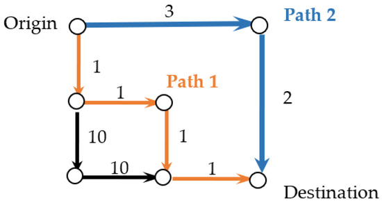
Figure 1.
Illustration transportation network.
Under this circumstance, the link travel time correlations, waiting times at signalized intersections and TTR are considered as the components of effective travel time (ETT). Moreover, we refer to TTR as the probability that travelers can arrive at their destination node on time [4]. TTR is an increasing concern for travelers because it allows travelers to make better use of their own time. As such, consideration of TTR induced by network uncertainty has become an important issue for transportation planning and modeling. On this basis, this paper proposes a new TRUE traffic assignment model. The remainder of this paper is organized as follows. Section 2 gives the assumptions and proposes an optimization model. The existence analysis of the solution is proved in Section 3. In Section 4, the solution algorithm and flow chart of the proposed model are given. The experimental results are shown and analyzed in Section 5. Finally, the conclusions are depicted in Section 6.
2. Model Assumptions and Model Establishment
2.1. Model Assumptions
- (1)
- It is assumed that OD demand and link flow follow normal distribution [6].
- (2)
- It is assumed that the link travel times and waiting times at signalized intersections are non-negative and follow a multivariate normal distribution [7,10,26].
- (3)
- It is assumed that the variation coefficient of OD demand in the traffic network is the same as the variation coefficient of path flow.
2.2. Model Establishment
2.2.1. Probability Distribution of Traffic Flow
The transportation network is denoted as , and and denote the origin node and destination node. represents the set of OD pair , and is a subset of . represents the nonempty path set. Then, we assumed that is a stochastic variable:
where is the mean value of OD demand, , is a stochastic variable and . Let be the standard deviation of the OD traffic demand, which is assumed to be a continuous nondecreasing function with respect to the mean OD demand.
Then, define the variation coefficient of OD demand as:
According to the flow conservation equation, it can be written as follows:
where represents the path flow , is link flow , and are random variables and is a variable in the incidence matrix, which is expressed as: if link belongs to the path , then , otherwise, . We assume and , and then the following equations can be obtained according to Equations (4)–(6):
The standard deviations of path flow and link flow can be deduced as:
According to Asakura and Kashiwadani [4], Chen et al. [27] and the assumptions (1) in Section 2.1, the probability distribution formula of traffic flow can be obtained as follows:
2.2.2. Probability Distributions of Link and Path Travel Time
In this section, the link travel time is regarded as a strictly increasing function of the link flow:
where represents the link travel time and represents the function of the link travel time.
Then, the mean and variance of the link travel time are:
where represents the mean link travel time, represents the standard deviation of link travel time and represents the probability density function of link flow.
According to the Assumption (1) in Section 2.1 and Equation (12), can be expressed as follows:
In this paper, the BPR function is employed to depict , and Equation (15) can be showed as below:
According to Shao et al. [6], the mean and variance of the corresponding link travel time can be obtained:
The detailed derivation process is referred to Shao et al. [6].
The path travel time can be obtained as below:
By using the central limit theorem, it can be deduced that the path travel time also follows normal distribution [26,28] according to some traditional works of research and assumptions in Section 2.1. On the basis of Zhang et al. [8] and Shen et al. [10], the travel time correlations among different links exist in real transportation networks. Under this circumstance, the mean and variance of link travel times are shown as below:
2.2.3. Waiting Time at Signalized Intersections
The shortest reliable path problem is usually regarded as a path with the shortest time corresponding to a definite OD pair (considering TTR). Meanwhile, the delays due to traffic lights at intersections are often ignored in the shortest reliable path problem. However, in most real-world transportation networks, the distance between links (the time to pass links) is relatively short, so the waiting time at signalized intersections often occupies a significant component of path travel time, especially in congested road networks. Therefore, it is not optimal to consider only the path with the shortest distance (ignoring the waiting time at signalized intersections) in real transportation networks. Therefore, according to Assumption (2) and Shen et al. [10], the mean value and standard deviation of node intersection delays are depicted as and . Further, the distribution of path intersection delays (sum of node intersection delays) is also approximated by normal distribution. Under this circumstance, Equations (25) and (26) represent the mean () and standard deviation () of path intersection delays and can be obtained on the basis of the properties of normal distribution. Under this circumstance, the mean and standard deviation of path intersection delays can be obtained as follows:
According to Shen et al. [10], the symbol is adopted to represent a location variable regarding the node–node incidence relationship. means that node is on the top of node , node is at the bottom of node , node is on the left side of node and node is on the right side of node . The turning directions at a signalized intersection means that turning is allowed at point . The turning variable at a signalized intersection includes three directions: turn left, go straight and turn right. Specific definitions are as follows:
On the basis of Equation (11) and values of , the values of can be obtained. Specifically, if and , the movement (Figure 2). According to Equation (27), represents the movement of a left turn, represents going straight and represents the movement of a right turn. The rest can be performed in the same manner.
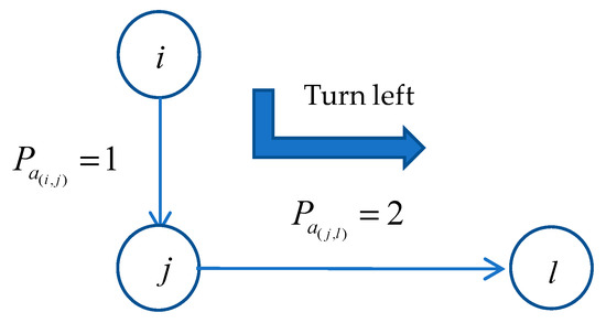
Figure 2.
The diagram for turn left.
2.2.4. The Path Effective Travel Time
According to Shen et al. [7] and Chen et al. [26], the effective path travel time can be calculated as below:
The safety margin is usually determined by the following model:
In this paper, we assumed that the path travel time follows normal distribution, so Equation (28) can be transformed into the following form through a simple transformation:
where is the inverse function of the cumulative probability function with confidence level . Considering the correlations and DITS, the following new expression can be obtained (see Shen et al. [10] for details) while incorporating Equations (23)–(27) into the ETT (Equation (30)), as below:
where represents the ETT of the reliable path considering the correlations and DITS. The Equation (31) consists of three parts, the mean path travel time, the mean path intersection delays and safety margin (with SD of link travel time, SD of node intersection delays and link travel time correlations). It should be noted that the link travel time correlations and delays at signalized intersections are not considered in the conventional reliability-based traffic assignment model. Then, the proposed new ETT is adopted to the conventional reliability-based traffic assignment model. Further, the proposed model is transformed into a variational inequality (VI) model.
3. Analysis of the Existence of Solutions
According to Shao et al. [6], it can be seen that when travelers make path selection in a transportation network, they usually choose the path with the shortest ETT. Thus, when the traffic assignment model presented in Section 2 reaches equilibrium, the following mathematical model can be obtained:
where denotes the path ETT when the traffic network reaches equilibrium.
In terms of the traffic assignment model presented in Section 2 and Equation (32), it could be converted into a variational inequality problem (VIP), that is, finding such that
where represents a constraint set of the above constraint optimization problem, which satisfies the following conditions:
Theorem 1.
The VIP (33)–(35) has at least one solution.
Proof.
For convenience, we denote , and as the vectors , and , respectively. First, it is obvious that is continuous with respect to and . Second, constraint set is compact and convex. According to Facchine and Pang [29], we can obtain that the VIP (33)–(35) has at least one solution. □
Theorem 2.
The solution of the VIP (33)–(35) is equivalent to the condition (32) of the model presented in Section 2.
Proof.
To ensure that ETT is positive, we suppose that which is the assumption about the heuristic algorithm presented in Shao et al. [6]. According to Dafermos [30], the classical proof for the equivalence can also be used in the proposed model in Section 2. □
4. Algorithm Design
The proposed model has certain specificity, i.e., the ETT in the proposed model is nonadditive due to the fact that travel time correlations and reliability are considered. Therefore, some traditional methods for solving a traffic assignment problem cannot be directly used. The algorithm based on the heuristic algorithm proposed in Shen et al. [9,10] and the method of successive average (MSA) [31] is proposed.
4.1. Algorithm Steps
By using the MSA to solve the proposed TRUE-CD, we find that the more the feasible paths, the higher the complexity of the algorithm. Under this circumstance, the algorithm proposed in this section takes the column generation method (CGM) into account, which can greatly reduce the number of path sets and simplify the calculations. Additionally, the traditional path-finding algorithms still suffer the difficulties that the paths with minimum ETT need to be found in each iteration and the ETT satisfies nonadditive property. To overcome these difficulties and solve the proposed model more efficiently, the heuristic algorithm proposed in Shen et al. [9,10] will be used in this paper to solve this problem. In order to verify whether the model achieves the equilibrium condition, the stop criterion from the research of Shao et al. [32] is adopted to verify the equilibrium condition. The detailed steps are described as below:
Step 1: Input: confidence level ; the parameters and of BPR function; link free-flow travel time ; link capacity , and ; the correlation coefficient ; node position matrix ; and tolerance of stop criterion .
Step 2: Calculate the shortest path set (without traffic flow): Under the assumption that there is no traffic flow on any links, then the additive property of link travel time holds. Furthermore, the K-shortest path algorithm and the link free-flow travel time can be used to calculate the shortest path for each OD pair. Then, put them into a path set.
Step 3: Traffic assignment: The all-or-nothing method is adopted to assign the flow to the current path set for each OD pair.
Step 4: Calculate the reliable shortest path set: Calculate the reliable paths and ETT for each OD pair using the heuristic algorithm proposed in Shen et al. [9,10] and generate a new set of paths using the column generation algorithm.
Step 5: Update the step size:
Step 6: Update path flow (iterative direction):, where:
Step 7: Stop criterion: , where:
If the stop criterion is satisfied, terminate the iteration. Otherwise, go to step 4.
4.2. The Flowchart of the Heuristic Algorithm
In order to show the detailed process of the algorithm more visually, the following flow chart of the proposed algorithm is created according to the steps of the algorithm in Section 4.1 (Figure 3).
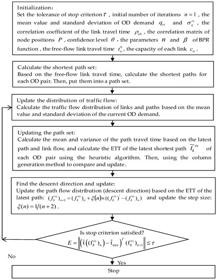
Figure 3.
The flowchart of the heuristic algorithm [9,10].
5. Numerical Examples
In this paper, a small traffic network (with 6 nodes and 7 links) and a medium-sized transportation network (24 nodes and 76 links) are adopted to demonstrate the performance of the proposed TRUE-CD model and MSA algorithm. The numerical experiments are performed using MATLAB R2020a on the Windows 10 platform running on a PC with an Intel Core (TM) i7-6500U 2.5 GHz CPU and 4 GB of memory.
5.1. A Small Traffic Network
This section adopts a small traffic network (Figure 4) to illustrate the properties of the proposed TRUE-CD model and algorithm in application. The OD demand is determined as below:
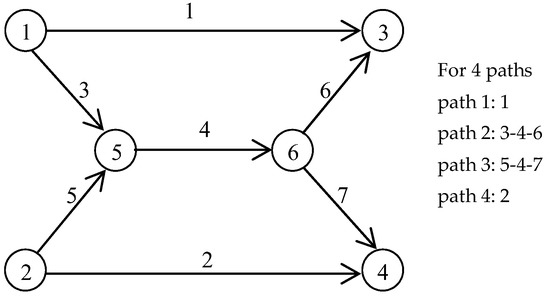
Figure 4.
A small transportation network.
It is assumed that the covariance matrix of link travel time is randomly generated and is consistent with the variance of link travel time. Suppose that the waiting times at signalized intersections follow normal distribution [10]:
where (1.5 denotes the MTT of turning left (minute), 1 denotes the MTT of going straight (minute), 0.1 denotes the MTT of turning right (minute)), (0.5 represents the variance travel time of turning left (minute), 0.25 represents the variance travel time of going straight (minute) and 0.05 represents the variance travel time of turning right (minute)). It is assumed that from link 3 to link 4, one needs to turn left at node 5; from link 5 to link 4, one needs to turn right at node 5; from link 4 to link 6, one needs to turn left at node 6; from link 4 to link 6, one needs to turn right at node 6. Other parameters can refer to Shao et al. [32].
5.2. Analysis of Effective Travel Time
In order to show the influence of the correlations and DITS on path travel time, this section mainly calculates the ETT of path 2 under different conditions. The detailed results are shown in Figure 4.
The ETT of path 2 under two different scenarios (Scenario A: with consideration of travel time correlations; Scenario B: with consideration of travel time correlations and waiting time at signalized intersections) are shown in Figure 5. For Scenario A (the top graph in Figure 5), it can be found that when the OD demand is low, the ETT is almost the same as MTT. Particularly, when the OD demand level is less than 15, the ETT is equal to the MTT. Generally, the MTT is a main factor affecting travelers’ path choice when OD demand is low. Moreover, it can be found that when the OD demand increasing, the ETT also increasing. The growth rate of the safety margin is obviously faster than the MTT. Under this circumstance, it can be concluded that higher OD demand is more likely to cause greater randomness of traffic network (stochastic travel time). For Scenario B (the graph below in Figure 5): when the OD demand is low, it can be found that the ETT is not equal to the MTT. This is because when the OD demand is low, Scenario B also considers the waiting time at signalized intersections. Regardless of whether the OD demand on path 2 is low or high, it is imperative to consider the intersection delays when passing through the signalized intersections. Moreover, when the OD demand is low, the difference between the ETT and the MTT is equal to the DITS.
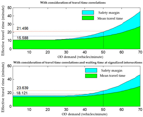
Figure 5.
The ETT of path 2 with different values of OD demand under two different cases.
In terms of Figure 5, when the OD demand is equal to 50 vehicles/minute, the ETT in Scenario A is 21.456 min and the MTT is 15.588 min. For Scenario B, the ETT is 23.639 min and the MTT is 18.121 min. It can be obtained that the waiting time at signalized intersections occupies an important part of the ETT. The traveler will underestimate the ETT or miss some important meetings if the waiting time at signalized intersection is not considered.
The above discussion verifies that when the OD demand is relatively large, the safety margin will become an important reference when selecting the path.
5.2.1. Comparisons between the Proposed Model and the Existing Models
To better illustrate the proposed model in this paper, we compare the two existing models (UE and TRUE model proposed in Shao et al. [32]) with the proposed TRUE-CD in this manuscript (two scenarios, the TRUE model considering the correlations (TRUE-C) and the TRUE model considering both the correlations and DITS (TRUE-CD)). The detailed results are shown in Figure 6.
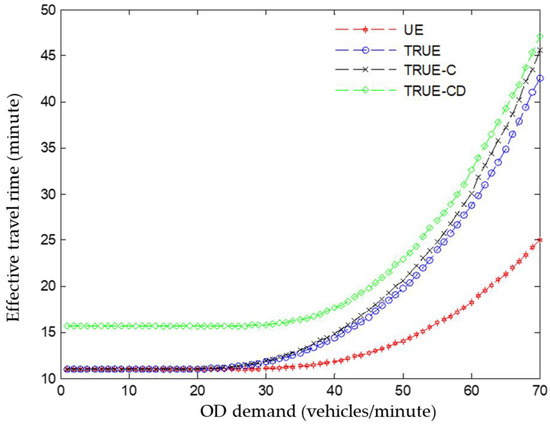
Figure 6.
The comparisons between the existing model and proposed model (the ETT of path 2).
According to Figure 6, it can be found that the ETT of path 2 is different under different models and OD demand. When the OD demand is low, the ETT of the model UE, TRUE and TRUE-C are equal. It is because when the OD demand is relatively low, almost all traffic flow is allocated to path 1 (with less ETT). Under this circumstance, the ETT of path 2 is the free-flow travel time with the absence of traffic flow. However, with the OD demand increasing, the ETT of path 2 in models UE, TRUE and TRUE-C is also increasing rapidly. It can be seen from Figure 6 that TRUE-C has the fastest growth rate due to the fact that the TRUE-C model considers not only the TTR but also the link travel time correlations. Therefore, the model TRUE-C may be more suitable for the traffic network with higher OD demand than the TRUE model. It also can be found from Figure 6 that the ETT of path 2 of the proposed model TRUE-CD is the most different from the other three models. Especially when the OD demand is low, the ETT of the proposed model TRUE-CD is longer than the other three models. This is because the proposed model TRUE-CD considers the waiting time at signalized intersections, which remains unchanged with different travel flow. Therefore, the extra time is the waiting time at signalized intersections.
Based on the above discussion, the model proposed in this paper can better estimate the ETT under different values of reliability. Moreover, it can more help travelers to choose a path accurately and avoid inconvenience caused by delays during the trip. If the travel time correlations and the waiting time at signalized intersections are not considered in ETT, the results will overestimate or underestimate the traveler’s travel time. Further, it will obtain inaccurate traffic assignment results. Under this circumstance, it can be concluded that the proposed TRUE-CD model in this paper is more suitable for traffic networks under various OD demand levels, especially with high OD demand.
5.2.2. Comparison of Traffic Flow in TRUE and TRUE-CD Models
In order to illustrate the characteristics of path flow distribution in the proposed model TRUE-CD, the traffic flow of paths 1 and 2 in OD pair 1 is adopted. The detailed results are shown in Figure 7.
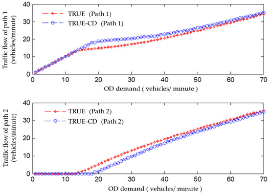
Figure 7.
The comparison between TRUE and TRUE-CD under different values of OD demand for OD pair 1.
It can be found that when the OD demand level is relatively low, the path flow in TRUE and TRUE-CD models are similar. However, with the increase in OD demand, the gap between TRUE and TRUE-CD becomes larger and larger. Moreover, the MTT is a main factor affecting travelers’ path choice when OD demand is low. This is because when the OD demand level is very low, the other part of the ETT (safety margin) is also relatively low, which can be ignored at this stage. However, it can be seen from Figure 6 that TRUE and TRUE-CD have completely different ETTs when OD demand is low due to the waiting time at signalized intersections. In addition, when the OD demand level is high, travelers need to consider the values of safety margin to ensure that they can arrive at the destination node on time. Therefore, it can be concluded that the proposed TRUE-CD model in this paper is more suitable for traffic networks under various OD demand levels.
5.2.3. Effects of Different OD Demand and TTR on Effective Travel Time
In this paper, we refer to TTR as the probability that travelers can arrive at their destination node on time [4]. Using the on-time arrival probability, the travelers’ risk attitudes toward travel time uncertainty can be identified by the following three types [9]: risk-averse (), risk-neutral () and risk-seeking (). In this paper, we only consider the nontrivial case of risk-averse behaviors; hence, the associated on-time arrival probability is greater than 50%. In order to illustrate the impact of different OD demand and TTR on the ETT, this section divides the travelers into five levels according to TTR, from 50%, 60%, 70%, 80% and 90%, respectively. Under this circumstance, the 50%, 60%, 70%, 80% and 90% TTR represent the probability that a traveler can arrive at the destination within a given travel time threshold [4]. Moreover, the OD demand changes from 1 to 70 (increasing by 1). Accordingly, the ETT of path 2 in OD pair 1–3 under different OD demand and reliability is depicted in Figure 8. From Figure 8, when the OD demand is low, the ETT is approximately equal to the MTT (that is, ). Under this circumstance, the OD demand changes little, and travelers only need to estimate a small safety margin to improve the TTR.
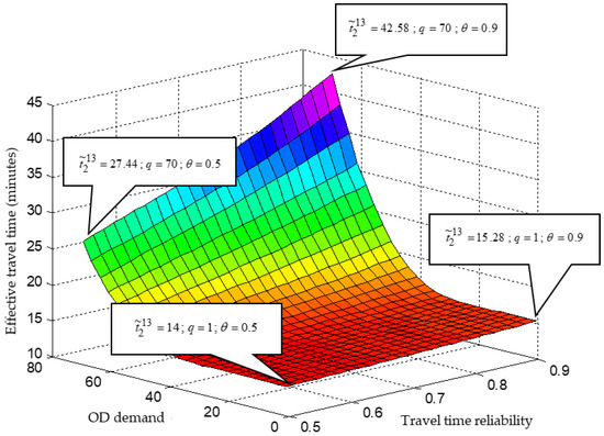
Figure 8.
The ETT of path 2 between OD pair 1–3 under different values of OD demand and reliability.
At this time, the main factor affecting the travelers’ path selection is the MTT. For example, when the OD demand level is 1 vehicle/minute, the ETT is 15.28 min if a traveler wants to guarantee more than 90% reliability. However, if the traveler only wants to guarantee 50% reliability, this ETT becomes 14 min. However, when OD demand levels are high, the ETT increases rapidly, especially for high-reliability requirements (the leftmost curve in Figure 8). As discussed before, higher OD demand levels lead to higher traffic flow variations. Under this circumstance, the travel time becomes more random. Then, travelers need to estimate more values of safety margin to improve the TTR. Therefore, when the OD demand level increases, the ETT will also increase quickly.
Meanwhile, it can be found that a higher value of confidence level (TTR) will lead to an increase in ETT. This is because when travelers consider higher TTR, they will need to estimate ETT more accurately. For instance, if the traveler wants to guarantee more than 90% reliability, the ETT is 42.58 min when the OD demand is 70 vehicles/min. However, if the traveler only wants to guarantee 50% reliability, then the ETT will become 27.44 min.
5.3. A Medium-Sized Transportation Network
In order to show the effectiveness of the proposed TRUE-CD model and the MSA algorithm, a medium-sized transportation network (Figure 9) is adopted. It consists of 24 nodes and 76 links. Suppose that there are 96 OD pairs in the transportation network (Table 1), the TTR is set to be 95% and the stopping criterion for iteration is regarded . Other parameters of the BPR function can be set and refer to Shao et al. [6]. The mean demand of all OD pairs are assumed to be 300 vehicles/hour. Moreover, the standard deviation of OD demand in this experiment is set as follows:
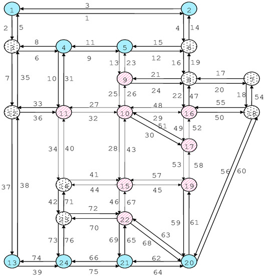
Figure 9.
Sioux Falls transportation network.

Table 1.
The OD pairs and results of Sioux Falls.
According to the proposed algorithm, it is found that the solution of the TRUE-CD model can be obtained after 850 iterations. As shown in Figure 10, the proposed algorithm in this paper is generally convergent. However, the convergence error of the algorithm (see Equation (38)) does not decrease monotonically due to the idea of MSA. From this point, it can be found that it is difficult to determine or explain the monotonicity of VI model of the proposed TRUE-CD for the moment, which will lead to failure to determine the descent direction and appropriate step size of the iteration. In order to illustrate the equilibrium conditions of the proposed model, the results of OD pair (8,3) are shown in Table 1. On the basis of the results as shown in Table 1, when the traffic network reaches equilibrium, the ETT of path 21-25-27-31-8 (link sequence) and 19-14-3-2 (link sequence) are the same, which is consistent with the definition of equilibrium condition. Therefore, it can be concluded that the proposed algorithm can be applied to find the solutions of the proposed TRUE-CD model for medium-scale traffic networks.
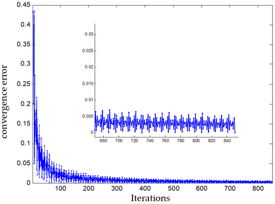
Figure 10.
Algorithm convergence.
5.4. Algorithm Analysis
- (1)
- The first step of the algorithm in this paper is to input some basic parameters of the proposed model.
- (2)
- In the second step of the proposed algorithm, the shortest path algorithm (e.g., Dijkstra Algorithm) can be adopted to find the shortest path between each OD pair and put them into a path set under the condition of no traffic flow in transportation networks. The algorithm complexity of this step is .
- (3)
- The traffic flow of the OD pair is allocated to the set of paths obtained in the second step with the all-or-nothing criterion in the third step of the proposed algorithm.
- (4)
- On the basis of Shen et al. [9,10], the reliable path and the corresponding ETT can be obtained in the fourth step of the proposed algorithm.
- (5)
- In the fifth and sixth steps, the MSA algorithm and Equations (36) and (37) are used to update the step size and iterative direction. According to previous studies [32], it can be found that the MSA algorithm is a forced convergence algorithm.
- (6)
- The stopping criterion is shown in the seventh step in order to determine when to stop the iteration of the proposed algorithm.
It can be seen from the above steps that the algorithm can determine the step size by adopting the MSA method (step size is ). Moreover, the proposed algorithm is bound to converge due to the property of forced convergence. However, convergence to the global optimal solution cannot be guaranteed.
6. Conclusions
The traffic assignment problem is the last stage of the classic ‘four-stage method’ of traffic planning. As a consequence, the traffic flow distribution plays a significant role in the accuracy of traffic flow analysis and prediction of highway projects. Moreover, the essence of the urban traffic congestion problem lies in the path choice behavior of travelers. In order to alleviate the traffic congestion problem quickly and effectively, we need to understand deeply and estimate the path choice behavior of travelers accurately. However, the traditional UE model regards the MTT as the standard for travelers to choose the path. In fact, due to many uncertain factors in the transportation network (e.g., weather condition, traffic accident), travelers’ daily travel time is stochastic. On this basis, this paper proposes a new travel time reliability-based user equilibrium (TRUE) traffic assignment model (with consideration of the travel time correlations and the waiting time at signalized intersections, TRUE-CD). Due to the stochastic nature of OD demand, the link travel time will be regarded as a stochastic variable in the manuscript. Although the travel time can be obtained based on the travelers’ daily travel experience, the travelers should not only consider the MTT but also the TTR. As a consequence, the ETT (sum of MTT and safety margin) is adopted to depict the TTR. It should be noted that the waiting time at signalized intersections and the travel time correlations cannot be ignored in the proposed model. Therefore, the new ETT with consideration of the travel time correlations and waiting time at signalized intersections is adopted in the new traffic assignment problem. When the new ETT is used as the basis for travelers to choose a path, the proposed TRUE-CD model can be transformed into a VI problem and give the proof of the existence of solutions. The model presented in this paper can be regarded as a generalization of the existing reliability-based traffic assignment model. Meanwhile, according to the numerical examples in Section 5, it can be seen that the proposed TRUE-CD model is more suitable for traffic networks with high OD demand. Therefore, the proposed model plays an important role in the light-controlled intersections or the transport network. Additionally, it can also help managers to estimate the path selection behavior of travelers more accurately and efficiently.
Several directions for research are worth further investigation: (1) How to design a more effective algorithm to solve the proposed TRUE-CD model, which can be improved in two aspects: (a) applying a reinforcement learning method to find the optimal reliable path and the corresponding ETT; (b) researching the monotonicity of the proposed model and find out more suitable descent direction and step length. (2) How to extend the proposed static TRUE-CD model to the dynamic traffic network assignment problem [33]. (3) Future works can extend our proposed algorithm based on multivariate normal distributed path travel times and delays at road intersections to generally distributed distributions to meet the demands from emerging data analytics research in transportation.
Author Contributions
Conceptualization, L.S. and Z.W.; methodology, L.S. and F.W.; software, L.S. and F.W.; validation, L.S.; writing—original draft preparation, X.L. and Y.C.; data curation, F.W.; writing—review and editing, L.S., F.W. and Y.C.; visualization, L.S. and X.L.; supervision, L.S. and F.W.; project administration, L.S.; funding acquisition, L.S. All authors have read and agreed to the published version of the manuscript.
Funding
This research was supported by the Humanities and Social Sciences Youth Foundation, the Ministry of Education of the People’s Republic of China (Project No. 22YJCZH144), the Postdoctoral Research Foundation of China (Project No. 2022M712680), the General Project of Natural Science Foundation of Colleges and Universities in Jiangsu Province (Project No. 22KJB110027) and the Initiation Foundation of Xuzhou Medical University (D2019046).
Institutional Review Board Statement
Not applicable.
Informed Consent Statement
Not applicable.
Data Availability Statement
These data will be available upon requesting the first author.
Conflicts of Interest
The authors declare no conflict of interest.
References
- Lo, H.K.; Tung, Y.K. Network with degradable links: Capacity analysis and design. Transp. Res. Part B 2003, 37, 345–363. [Google Scholar] [CrossRef]
- Lo, H.K.; Luo, X.W.; Siu, B.W.Y. Degradable transport network: Travel time budget of travelers with heterogeneous risk aversion. Transp. Res. Part B 2006, 40, 792–806. [Google Scholar] [CrossRef]
- Chen, A.; Yang, H.; Lo, H.K.; Tang, W.H. Capacity reliability of a road network: An assessment methodology and numerical results. Transp. Res. Part B 2002, 36, 225–252. [Google Scholar] [CrossRef]
- Asakura, Y.; Kashiwadani, M. Road network reliability caused by daily fluctuation of traffic flow. Eur. Transp. Highw. Plan. 1991, 19, 73–84. [Google Scholar]
- Clark, S.; Watling, D. Modeling network travel time reliability under stochastic demand. Transp. Res. Part B 2005, 39, 119–140. [Google Scholar] [CrossRef]
- Shao, H.; Lam, W.H.K.; Tam, M.L. A reliability-based stochastic traffic assignment model for network with multiple user classes under uncertainty in demand. Netw. Spat. Econ. 2006, 6, 173–204. [Google Scholar] [CrossRef]
- Zeng, W.L.; Miwa, T.; Wakita, Y.; Morikawa, T. Application of Lagrangian relaxation approach to -reliable path finding in stochastic networks with correlated link travel times. Transp. Res. Part C 2015, 56, 309–334. [Google Scholar] [CrossRef]
- Zhang, Y.L.; Shen, Z.J.M.; Song, S.J. Lagrangian relaxation for the reliable shortest path problem with correlated link travel times. Transp. Res. Part B 2017, 104, 501–521. [Google Scholar] [CrossRef]
- Shen, L.; Shao, H.; Wu, T.; Lam, W.H.K.; Zhu, E.C. An energy-efficient reliable path finding algorithm for stochastic road networks with electric vehicles. Transp. Res. Part C 2019, 102, 450–473. [Google Scholar] [CrossRef]
- Shen, L.; Shao, H.; Wu, T.; Fainman, E.Z.; Lam, W.H.K. Finding the reliable shortest path with correlated link travel times in signalized traffic networks under uncertainty. Transp. Res. Part E 2020, 144, 102159. [Google Scholar] [CrossRef]
- Cantarella, G.E. A general fixed-point approach to multi-mode multi-user equilibrium assignment with elastic demand. Transp. Sci. 1997, 31, 107–128. [Google Scholar] [CrossRef]
- Xiong, Z.H.; Shao, C.F. Evaluation on the travel trait of road network under day-to-day stochastic demand-travel time reliability. J. Transp. Eng. Inf. 2006, 4, 40–44. (In Chinese) [Google Scholar]
- Kuang, A.W.; Huang, Z.X. On the Service Reliability in Stochastic Supply and Demand. Syst. Eng. 2007, 25, 25–30. (In Chinese) [Google Scholar]
- Cheng, L.; Li, Q.; Wang, J. Urban street network capacity reliability. J. Southeast Univ. 2004, 20, 235–239. [Google Scholar]
- Cantarella, G.E.; de Luca, S.; Cartenì, A. Stochastic equilibrium assignment with variable demand: Theoretical and implementation. Eur. J. Oper. Res. 2015, 241, 330–347. [Google Scholar] [CrossRef]
- Cantarella, G.E.; de Luca, S.; Di Gangi, M.; Di Pace, R. Approaches for solving the stochastic equilibrium assignment with variable demand: Internal vs. external solution algorithms. Optim. Methods Softw. 2015, 30, 338–364. [Google Scholar] [CrossRef]
- Chen, Q.; Pan, S.L. Direct formulation and algorithms for the probit-based stochastic user equilibrium traffic assignment problem. Transp. Plan. Technol. 2017, 40, 757–770. [Google Scholar] [CrossRef]
- Han, L.H.; Sun, H.J.; Wang, D.Z.W.; Zhu, C.J. A stochastic process traffic assignment model considering stochastic traffic demand. Transp. B Transp. Dyn. 2018, 6, 169–189. [Google Scholar] [CrossRef]
- Xu, J.X.; Guo, J.N.; Zhang, J. Research on traffic assignment model and algorithm based on cumulative prospect theory under uncertain factors. Transp. Res. Rec. 2021, 2675, 116–134. [Google Scholar] [CrossRef]
- Chen, A.; Zhou, Z. The alpha-reliable mean-excess traffic equilibrium model with stochastic travel times. Transp. Res. Part B 2010, 44, 493–513. [Google Scholar] [CrossRef]
- Wang, J.Y.T.; Ehrgott, M.; Chen, A. A bi-objective user equilibrium model of travel time reliability in a road network. Transp. Res. Part B 2014, 66, 4–15. [Google Scholar] [CrossRef]
- Shen, L.; Shao, H.; Li, C.J.; Sun, W.W.; Shao, F. Modeling stochastic overload delay in a reliability-based transit assignment model. IEEE Access 2019, 7, 3525–3533. [Google Scholar]
- Levin, M.W.; Duell, M.; Waller, S.T. Arrival time reliability in strategic user equilibrium. Netw. Spat. Econ. 2020, 20, 803–831. [Google Scholar] [CrossRef]
- Wang, S.; Lu, J.; Jiang, L.P. Time reliability of the maritime transportation networks for China’s crude oil imports. Sustainability 2020, 12, 198. [Google Scholar] [CrossRef]
- Jenelius, E.; Koutsopoulos, H.N. Travel time estimation for urban road networks using low frequency probe vehicle data. Transp. Res. Part B 2013, 53, 64–81. [Google Scholar] [CrossRef]
- Chen, B.Y.; Lam, W.H.K.; Li, Q.Q. Efficient solution algorithm for finding spatially dependent reliable shortest path in road networks. J. Adv. Transp. 2016, 50, 1413–1431. [Google Scholar] [CrossRef]
- Chen, A.; Subprasom, K.; Ji, Z.W. Mean-variance model for the build-operate-transfer scheme under demand uncertainty. Transp. Res. Rec. 2003, 1857, 93–101. [Google Scholar] [CrossRef]
- Srinivasan, K.K.; Prakash, A.A.; Seshadri, R. Finding most reliable paths on networks with correlated and shifted log-normal travel times. Transp. Res. Part B 2014, 66, 110–128. [Google Scholar] [CrossRef]
- Facchinei, F.; Pang, J.S. Finite-Dimensional Variational Inequalities and Complementarity Problems; Springer: New York, NY, USA, 2003. [Google Scholar]
- Dafermos, S. The general multimodal network equilibrium problem with elastic demand. Networks 1982, 12, 57–72. [Google Scholar] [CrossRef]
- Sheffii, Y. Urban Transportation Networks: Equilibrium Analysis with Mathematical Programming Models; Prentice-Hall, Inc.: Englewood Cliffs, NJ, USA, 1985; pp. 18–104. [Google Scholar]
- Shao, H.; Lam, W.H.K.; Meng, Q.; Tam, M.L. Travel time reliability-based traffic assignment problem. J. Manag. Sci. China 2009, 12, 27–35. (In Chinese) [Google Scholar]
- Mao, X.H.; Wang, J.W.; Yuan, C.W.; Yu, W.; Gan, J.H. A dynamic traffic assignment model for the sustainability of pavement performance. Sustainability 2019, 11, 170. [Google Scholar] [CrossRef]


Publisher’s Note: MDPI stays neutral with regard to jurisdictional claims in published maps and institutional affiliations. |
© 2022 by the authors. Licensee MDPI, Basel, Switzerland. This article is an open access article distributed under the terms and conditions of the Creative Commons Attribution (CC BY) license (https://creativecommons.org/licenses/by/4.0/).