About Calculation and Forecast of Temperature in the Layer Cell of Self-Heating of Raw Materials in a Silo

Abstract

The article clarifies an approximate variant for calculating the temperature in an inhomogeneous layer cell without a clear boundary under the assumption of significant distance in its center between the upper and lower ends of the silo when heat exchange conditions have little effect on the development of temperature in the layer cell due to poor thermal conductivity. The normal Gaussian law concerning distribution of thermal sources in the cell on an axis of a silo is accepted. The integral cosine of the Fourier transform is used to construct the analytical solution of the nonstationary thermal conductivity problem. A compact formula for calculating the increase in excess temperature in the center of the self-heating cell over time is derived and used to identify the parameters of the cell. The change in temperature at other points of the raw material is expressed through incomplete gamma function that is reduced to the probability integral. Calculations show that for the selected distribution of thermal sources, the temperature increase slows down rapidly with separation from the center of the cell. The possibility of determining the pattern distribution of the localized field of excess ambient temperature over time is proved. Examples of density identification of thermal sources are given. After identification, the calculation formulas become consistent with the experiment and suitable for the theoretical prediction of temperature rise in the raw material. The approbation of the proposed mathematical expressions to identify the parameters of the self-heating process of raw materials showed high accuracy relative to experimental data with a deviation of 0.01–0.015%. It is possible not only to determine the parameters of the self-heating cell but also to predict the time of reaching a flammable temperature in it.

1. Introduction

For the self-heating of vegetable raw materials, worsening storage conditions lead to quality loss. There are cases when self-heating was the cause of fires in storage [1].

In this case, it becomes not only harmful but also dangerous to the environment. Therefore, this phenomenon has long been studied from different positions [1,2,3,4]. To prevent emergencies, thermal control systems are used, which control the dynamics of temperature regimes based on theoretical models. The latter allows us to predict the development of the temperature of raw materials and calculate the time required to reach a fire-hazardous temperature regime, which is the prevention of emergencies. In particular, various systems of thermal control of raw materials and the analysis of the composition of the gaseous medium adjacent to the raw materials are used [5,6,7,8]. Optical research methods are also used. One of the main characteristics of the process of self-heating is the change in time of its temperature field. Therefore, much attention is paid to this issue.

The use of mathematical modeling to study the mechanisms of heat transfer in a liquid (nano-liquid) moving between rotating discs is given in [9]. Using the model made it possible to determine process parameters without conducting experimental tests.

In work [10], the flow is studied under the influence of space- and temperature-reliant heat source/sinks, viscous dissipation, and ohmic heating on stretching/shrinking surfaces embedded in a porous medium.

As justified in work [9,10,11], similarity transformations are utilized to transcribe the momentum and thermal equations in non-dimensional form.

The theoretical models developed in [1,12] are based on the solutions of direct problems of nonstationary thermal conductivity. To perform calculations, they need information about the parameters (thermophysical characteristics) of internal thermal sources (self-heating cells). In practice, such information is usually missing, because thermal control systems determine the temperature of raw materials at the points of its measurement.

Therefore, there is no correspondence between the measurement results and the input parameters of the theoretical models. To do this, it is necessary to eliminate the discrepancy (inconsistency) between the systems of technical thermal control and temperature forecasting systems. Therefore, the inverse problem of nonstationary thermal conductivity has to be solved. It consists of determining the parameters of the internal localized thermal source based on the results of temperature measurements at individual points of the raw material array.

In the development of mathematical models of thermal fields, certain forms of self-heating cells are distinguished as internal thermal sources. The most common of them are nest [13,14,15], layer [16,17], and rod [18,19,20]. Layer ones are among the most flammable [13]. Given this, here we study the temperature field of the layer cell without a clear boundary in the assumption that the distribution of thermal sources in it is subject to the normal Gaussian law. A similar technique was used in [16], but in contrast to this work, here we focus on the identification of the density of internal thermal sources and the forecast of temperature development, at least at the beginning of self-heating, when heat transfer and silo ends have little effect on temperature development in the remote self-heating center. Localization of excess temperature in the raw material is possible due to its weak thermal conductivity [21]. The study is based on the theoretical and experimental method, which was used in other works [13,16,21].

The aim of the present work is to derive formulas for identifying the parameters of the internal source of self-heating based on the results from the experimental measurement of the temperature of raw materials and subsequent forecast of temperature rise.

2. Methods for Determining the Internal Source of Self-Heating of Raw Materials

The distribution of excess temperature in the raw material along the axis of the silo (Figure 1) is described using the differential equation:

$$\frac{{\partial }^2{\rm T}}{\partial x^2}-\frac{1}{\alpha }\frac{\partial {\rm T}}{\partial t}=-\frac{q\left(x\right)}{\lambda F}H\left(t\right),$$

(1)

in which:

• x—the axial coordinate with the beginning in the center of the cell;
• t—time;
• $\alpha =\lambda /\left(\rho c\right)$—coefficient of thermal conductivity of raw materials;
• λ—its thermal conductivity coefficient;
• $\rho ,c$—respectively, the specific weight and specific heat of raw materials;
• F—cross-sectional area of the silo;
• H(t)—single Heaviside function;
• $q\left(x\right)$—linear density of thermal sources in the center of self-heating.

We define it using the expression:

$$q(x)=q_0\exp \left(-\frac{x^2}{R^2}\right),$$

(2)

where:

• $q_0=q(0)$—the maximum value of density;
• R—characterizes the rate of decrease of density in the x coordinate (along the axis of the silo).

Figure 1. Hearth in an endless array of grain.

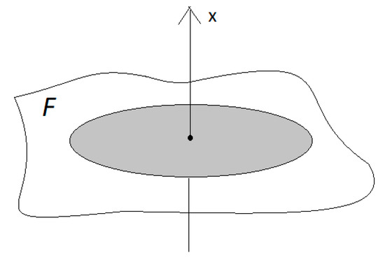
Figure 1. Hearth in an endless array of grain.

At the specified level of temperature calculation, the assumption is accepted that the reservoir center is significant in the distance in the center between the upper and lower ends of the silo. The minimal impact on the temperature development in the center of the cell under study due to the weak thermal conductivity of heterogeneous raw materials is taken into account. The expediency of using such assumptions is based on studies [5,12], where the dimensions of the silo are assumed to be infinite. This allows us to find a finite numerical solution to the equations.

Let us note that the distribution (2) in the layer cell was also used in [5,8], in [5] the thermal conductivity problem was solved using numerical methods, and in [16] trigonometric series were used.

To construct an analytical solution for Equation (1) under the initial condition: ${\rm T}\left(x,0\right)=0,$ use the integral cosine transformation with the parameter s:

$$\overline{f}(s)={\displaystyle \underset{0}{\overset{\infty }{\int }}f(x)\cos (}sx)dx; f(x)=\frac{2}{\pi }{\displaystyle \underset{0}{\overset{\infty }{\int }}\overline{f}(s)\cos (}sx)ds.$$

(3)

In space, the cosine of Equation (1) adopts the form at initial condition ${\rm T}\left(x,0\right)=0$:

$$\frac{\partial \overline{T}(s,t)}{\partial t}+\alpha s^2 \overline{T}(s,t)=a\overline{q}(s),$$

(4)

where, taking into account (2):

$$\overline{q}(s)=\frac{1}{\lambda F}{\displaystyle \underset{0}{\overset{\infty }{\int }}q(x)}\cos (sx)dx=\frac{q_0}{\lambda F}{\displaystyle \underset{0}{\overset{\infty }{\int }}\exp \left(-\frac{x^2}{R^2}\right)}\cos (sx)dx.$$

(5)

Using Table [22] instead of (5), we obtain:

$$\overline{q}(s)=\frac{q_{0}R}{2F\lambda }\sqrt{\pi }\exp \left(-\frac{R^2{s}^2}{4}\right).$$

(6)

The differential Equation (4) has the solution:

$$\overline{T}(s,t)=\frac{\overline{q}(s)}{s^2}\left[1-\exp (-a{s}^{2}t)\right],$$

(7)

which, taking into account (6), is reduced to the expression:

$$\overline{T}(s,t)=\frac{q_{0}R\sqrt{\pi }}{2\lambda F{s}^2}\left[1-\exp (-a{s}^{2}t)\right]\exp \left(-\frac{R^2{s}^2}{4}\right).$$

(8)

By reversing the transformation of the image $\overline{T}(s,t)$, we obtain the original:

$${\rm T}\left(x,t\right)=\frac{2}{\pi }\underset{0}{\overset{\infty }{{\displaystyle \int }}}\overline{T}\left(s,t\right)\mathit{cos}(sx)ds=\frac{q_{0}R}{\lambda F\sqrt{\pi }}\underset{0}{\overset{\infty }{{\displaystyle \int }}}\frac{1}{s^2}\left[1-\mathit{exp}(-a{s}^{2}t)\right]\mathit{exp}\left(-\frac{R^2{s}^2}{4}\right)\mathit{cos}(sx)ds.$$

(9)

From it, to calculate the maximum temperature in the center of the cell (x = 0), determine the formula:

$$T(0,t)=\frac{q_{0}R}{\lambda F\sqrt{\pi }}{\displaystyle \underset{0}{\overset{\infty }{\int }}\frac{1}{s^2}}\left[\exp \left(-\frac{R^2{s}^2}{4}\right)-\exp \left(-s^2\left(\frac{R^2}{4}+at\right)\right)\right]ds.$$

(10)

This integral refers to the table. Taking into account [19], we obtain a compact formula:

$$T(0,t)=\frac{q_{0}R}{2\lambda F}\left(\sqrt{R^2+4at}-R\right).$$

(11)

To obtain the expression $T(x,t)$ for $x>0$, we use the integral representation:

$$\frac{1}{s^2}\left[1-\exp (-a{s}^{2}t)\right]={\displaystyle \underset{0}{\overset{at}{\int }}\exp (-s^2}y)dy.$$

(12)

By substituting (12) for (9), we obtain:

$$T(x,t)=\frac{q_{0}R}{\lambda F\sqrt{\pi }}{\displaystyle \underset{0}{\overset{at}{\int }}{\displaystyle \underset{0}{\overset{\infty }{\int }}\exp \left[-s^2\left(y+\frac{R^2}{4}\right)\right]}}\cos (sx)dsdy.$$

(13)

Furthermore, taking into account that [19]:

$${\displaystyle \underset{0}{\overset{\infty }{\int }}{e}^{-\beta {\eta }^2}}\cos \left(\beta \eta \right)d\eta =\frac{1}{2}\frac{\sqrt{\pi }}{\sqrt{\beta }}\exp \left(-\frac{b^2}{4\beta }\right),$$

(14)

expression (13) is given in the form:

$$T(x,t)=\frac{q_{0}R}{2\lambda F}{\displaystyle \underset{0}{\overset{at}{\int }}\frac{1}{\sqrt{y+R^2/4}}}\exp \left(-\frac{x^2}{R^2+4y}\right)dy.$$

(15)

Let us move on to the new integration variable $u=\frac{1}{R^2+4y}$, then:

$$T(x,t)=\frac{q_{0}R}{4\lambda F}{\displaystyle \underset{\frac{1}{R^2+4at}}{\overset{\frac{1}{R^2}}{\int }}{u}^{-3/2}}\exp (-x^{2}u)du$$

(16)

This integral is expressed through an incomplete gamma function $\mathrm{\Gamma }(a,Z)$ [22]. According to the following tables:

$$T(x,t)=\frac{q_{0}R}{4\lambda F}\left|x\right|\left[\mathrm{\Gamma }\left(-\frac{1}{2},\frac{x^2}{R^2+4at}\right)-\mathrm{\Gamma }\left(-\frac{1}{2},\frac{x^2}{R^2}\right)\right].$$

(17)

Since [22] is

$$\mathrm{\Gamma }\left(-\frac{1}{2},Z\right)=\mathrm{\Gamma }\left(-\frac{1}{2}\right)+\frac{2}{\sqrt{Z}}-{\displaystyle \sum _{n=1}^{\infty }\frac{{(-1)}^n{Z}^{n-1/2}}{n!(n-1/2)}},$$

(18)

then from (17) we obtain the series:

$$T(x,t)=\frac{q_{0}R}{2\lambda F}\left\{\sqrt{R^2+4at}-R+{\displaystyle \sum _{n=1}^{\infty }\frac{{(-1)}^n{x}^{2n}}{n!(2n-1)}\left[\frac{1}{R^{2n-1}}-\frac{1}{{\left(\sqrt{R^2+4at}\right)}^{2n-1}}\right]}\right\}$$

(19)

This series has a fast convergence at $x<R.$ At $x=0$, Equation (11) follows from it.

Solution (17) can also be expressed in terms of the tabulated probability integral $\mathsf{\Phi }(Z)$ [23]. To perform this transformation, consider that [22]:

$$\mathrm{\Gamma }\left(-\frac{1}{2}Z\right)=\frac{2}{\sqrt{Z}}\exp \left(-Z\right)-2\mathrm{\Gamma }\left(\frac{1}{2},Z\right); \mathrm{\Gamma }\left(\frac{1}{2},Z^2\right)=\sqrt{\pi }-\sqrt{\pi }\mathsf{\Phi }(Z)$$

(20)

then:

$$\begin{array}{l}T(x,t)=\frac{q_{0}R}{2\lambda F}\left|x\right|\times \\ \times \left\{\frac{\sqrt{R^2+4at}}{\left|x\right|}\exp \left(-\frac{x^2}{R^2+4at}\right)-\frac{R}{\left|x\right|}\exp \left(-\frac{x^2}{R^2}\right)+\sqrt{\pi }\left[\mathsf{\Phi }\left(\frac{x}{\sqrt{R^2+4at}}\right)-\mathsf{\Phi }\left(\frac{x}{R}\right)\right]\right\} .\end{array}$$

(21)

In the case of missing tables of the probability integral with a smaller error 10⁻⁴, it can be calculated by the approximation formula [24]:

$$\mathsf{\Phi }\left(Z\right)=1-(a_1\zeta +a_2{\zeta }^2+a_3{\zeta }^3)\exp \left(-Z^2\right),$$

(22)

where:

$$a_1=0.348024; a_2=-0.095879; a_3=0.747856; \zeta =\frac{1}{1+0.47047\cdot Z.}$$

To use the resulting solutions in practical calculations, except thermophysical characteristics of the raw material, it is necessary to have the values $q_0$ and R. To do this, consider the method of their identification. Assume that the measurement results at $t=t_1$ at the moment of the cell temperature are $T(0,t_1)=T_1$ and at $t=t_2$ are $T(0,t_2)=T_2$.

Enter the designation: $\eta =T_2/T_1; \zeta =t_2/t_1; Z=4a{t}_1/R^2$ and use Equation (11). We obtain the equation:

$$\eta =\frac{\sqrt{1+Z\zeta }-1}{\sqrt{1+Z}-1}$$

(23)

It has the solution:

$$Z=4\frac{{\eta }^2(1+\zeta )-\eta \left({\eta }^2+\zeta \right)}{{\left({\eta }^2+\zeta \right)}^2-4\zeta {\eta }^2}$$

(24)

After calculating Z it is easy to find the parameters of the distribution of thermal sources in the cell, because:

$$R=2\sqrt{a{t}_1/Z}; q_0/F=\frac{2\lambda T_1}{R}{\left(\sqrt{R^2+4a{t}_1-R}\right)}^{-1}.$$

(25)

3. Numerical Results

For calculations with raw materials, we choose grass flour that has [5]: λ = 0.09 W/(mK); $\rho ,c$ = 8.5 × 10⁵ J·(m³K).

Example 1.

Let us calculate$T(0,t)$using Equation (11) when q₀/F = 75 W/m⁴. The obtained temperature values at different points in time are entered in the numerators of

Table 1. Values T(0,t) for different t.

t, Days	5	10	20	30
$T(0,t)$ °C	$\frac{14.137}{14.139}$	$\frac{21.380}{21.378}$	$\frac{37.721}{31.725}$	$\frac{39.688}{39.693}$

. Denominators are commonly known to be borrowed from [8].

The calculations obtained a pattern of changes in cell temperature T(0,t) in the raw material over time. It is established that in the range of up to 30 days, there is an intense increase in temperature in the center of the self-heating cell to 39.688 °C. This tendency to increase the temperature is characteristic of the physics of the corresponding processes of self-heating and is consistent with research experimental data for grass meal [5,24]. The obtained calculated values have a known minimum deviation (0.01–0.015%). This indicates the consistency of the results obtained using different methods and the high accuracy of the proposed method of calculation [25]. As you can see, the process of self-heating slows down the increase in excess temperature. For the practical implementation of the derived calculation formulas, in addition to the thermophysical characteristics of raw materials and characteristics of the silo, the required values of q₀ and R. They have to be identified using measurements of the excess temperature at the beginning of the self-heating.

The time boundary for reaching the critical cell temperature at which active gas evolution (from 100 °C) will begin is proportional to the product $\rho \times c$. Therefore, raw materials with low specific heat and density are difficult to store. Bran can be such a complex raw material [1]. The time boundary before the onset of dangerous temperatures will be much shorter than for other types of raw materials.

Thus, this example proves the ability not only to determine the parameters of the self-heating cell, but also to predict the time of reaching a flammable temperature in it.

Example 2.

The approbation of the developed mathematical expressions will also be carried out for the problem of determining the parameters of the self-heating cell of raw materials. We identify the parameters of the cell q₀ and R, if at t₁ = 5 days$T_1=20.4°\mathrm{C};$and at t₂ = 10 days$T_2=34.4°\mathrm{C}.$For them$\eta =1.6863; \zeta =2; 4a{t}_1=0.1830 m^2.$Substituting the specifiedƞand ζ using Equation (24), we obtain:${\rm Z}=2.0405,$and then, using Equation (25), we find R = 0.2994 m; q₀/F = 55.068 W/m⁴. Close to these values, R = 0.3 m and q₀/F = 55 W/m⁴ were used in solving the direct problem of thermal conductivity in [8] to obtain the T₁ and T₂ involved in identification.

Given the results of identification, Equation (11) provided a form suitable for the estimated forecast of temperature development in the center of the cell over time:

$$T(0,t)\approx 91.5964(\sqrt{0.08964+0.03659\cdot t}-0.2994)°\mathrm{C}.$$

(26)

Here, time t has the dimension of the day.

Substituting in (26) t = 5 and t = 10 days, we accordingly receive T₁ ≈ 20.4 °C and T₂ ≈ 34.4 °C, which justifies carrying out the identification.

The sufficient accuracy of the calculation results also indicates the possibility of using the developed mathematical expressions to determine the parameters of the self-heating of flat cells.

Example 3.

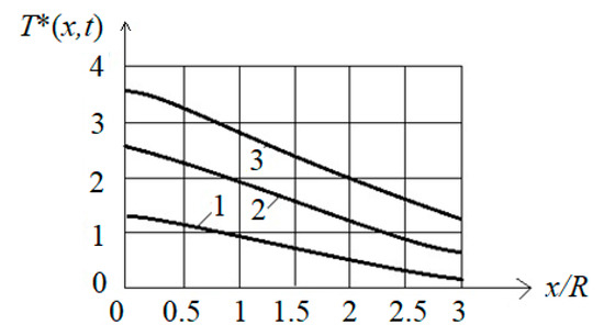
Using Equations (21) and (22), calculate the dimensionless temperature parameter$T\ast (x,t)=\frac{2\lambda F}{q_0{R}^2}T(x,t)$for different x and t. The results of its calculations at R = 0.4 m are graphically represented inFigure 2.

As you can see, the localized excess temperature field is expanding over time. For the selected initial data, we have a decrease in the temperature of self-heating of the cell by 2.3–4.2 times towards the periphery (ends) of the silo. Therefore, at the big t, the stated theory which does not consider heat exchange at the ends of the silo can lose force.

4. Conclusions

The derived calculation formulas are simple in practical implementation. They enable the identification of the density of the thermal sources in the cell and then become suitable for predicting the development of the temperature of the self-heating of raw materials over time. The calculations confirmed the adequacy of the obtained theoretical results.

The obtained analytical solution of the nonstationary thermal conductivity problem in combination with the experimental temperature measurement in the center of the self-heating cell facilitates the identification of the parameters of the internal thermal source and predicts the development of the self-heating temperature.

The solutions are convenient in the practical implementation of the theoretical and experimental method of calculation. They do not require special computer programs related to solving the inverse problem of thermal conductivity, which is related to mathematically incorrect problems.

References

- Karaiev, O.; Bondarenko, L.; Halko, S.; Miroshnyk, O.; Vershkov, O.; Karaieva, T.; Shchur, T.; Findura, P.; Prístavka, M. Mathematical modelling of the fruit-stone culture seeds calibration process using flat sieves. Acta Technol. Agric. 2021, 24, 119–123. [Google Scholar] [CrossRef]
- Havrylenko, Y.; Kholodniak, Y.; Halko, S.; Vershkov, O.; Miroshnyk, O.; Suprun, O.; Dereza, O.; Shchur, T.; Śrutek, M. Representation of a monotone curve by a contour with regular change in curvature. Entropy 2021, 23, 923. [Google Scholar] [CrossRef] [PubMed]
- Havrylenko, Y.; Kholodniak, Y.; Halko, S.; Vershkov, O.; Bondarenko, L.; Suprun, O.; Miroshnyk, O.; Shchur, T.; Śrutek, M.; Gackowska, M. Interpolation with specified error of a point series belonging to a monotone curve. Entropy 2021, 23, 493. [Google Scholar] [CrossRef] [PubMed]
- Khasawneh, A.; Qawaqzeh, M.; Kuchanskyy, V.; Rubanenko, O.; Miroshnyk, O.; Shchur, T.; Drechny, M. Optimal determination method of the transposition steps of an extra high voltage power transmission line. Energies 2021, 14, 6791. [Google Scholar] [CrossRef]
- Vogman, L.P.; Gorshkov, V.I.; Degtyarev, A.G. Fire Safety of Elevators; Stroyizdat: Moscow, Russia, 1993; p. 288. [Google Scholar]
- Sokolov, D.N. Assessment of the possibility of spontaneous combustion of grain in the silos of the elevator. In Innovative Technologies for the Production and Storage of Material Values for State Needs; Halley-Print: New York, NY, USA, 2017; pp. 284–287. [Google Scholar]
- Sukhareva, A.R.; Shukhanov, S.N. State of the issue of self-heating of grain mass in stacks. Bull. Orenbg. State Agrar. Univ. 2018, 3, 165–168. [Google Scholar]
- Orlikova, V.P.; Volynets, V.V. Study of focal spontaneous combustion of organic sub-stances. In Fire Safety: Problems, Ways of Improvement; Academy of Civil Protection of the Ministry of Emergency Situations: Moscow, Russia, 2019; pp. 169–177. [Google Scholar]
- Yaseen, M.; Rawat, S.K.; Kumar, M. Cattaneo–Christov heat flux model in Darcy–Forchheimer radiative flow of MoS2–SiO2/kerosene oil between two parallel rotating disks. J. Therm. Anal. Calorim. 2022, 147, 10865–10887. [Google Scholar] [CrossRef]
- Yaseen, M.; Rawat, S.K.; Kumar, M. Hybrid nanofluid (MoS2–SiO2/water) flow with viscous dissipation and Ohmic heating on an irregular variably thick convex/concave-shaped sheet in a porous medium. Heat Transf. 2022, 51, 789–817. [Google Scholar] [CrossRef]
- Yaseena, M.; Kumara, M.; Rawat, S.K. Assisting and opposing flow of a MHD hybrid nanofluid flow past a permeable moving surface with heat source/sink and thermal radiation. Partial Differ. Equ. Appl. Math. 2021, 4, 100168. [Google Scholar] [CrossRef]
- Sergunov, V.S. Remote Control of Grain Temperature during Storage; Agropromyzdat: Moskow, Russia, 1987; p. 174. [Google Scholar]
- Larin, A.N.; Olshanskiy, V.P.; Trigub, V.V. Problems of Non-Stationary Heat Conductivity in Self-Heating Raw Materials in Nesting Sources; KhNADU: Kharkov, Ukraine, 2003; p. 160. [Google Scholar]
- Olshanskii, V.P. Temperature field of cluster self-heating of bank in a silo. Combust. Explos. Shock Waves 2002, 38, 728–732. [Google Scholar] [CrossRef]
- Olshanskii, V.P.; Trigub, V.V. About the calculation of the temperature of self-heating of vegetable raw materials by a nesting spherical focus. In Bulletin of KhGPU. New Solutions in Modern Technologies; KhNADU: Kharkov, Ukraine, 2000; pp. 43–45. [Google Scholar]
- Eremenko, S.A.; Olshanskii, V.P. Problems of Non-Stationary Heat Conduction in Self-Heating Raw Materials Formation; KhNADU: Kharkov, Ukraine, 2003; p. 164. [Google Scholar]
- Olshanskii, V.P. Temperature field of bedded self-heating of a bank in a silo. Combust. Explos. Shock Waves 2001, 37, 53–56. [Google Scholar] [CrossRef]
- Abramov, Y.A.; Kirichkin, A.Y.; Otkidach, D.N. Mathematical model of the thermal field of grain embankment. Fire Explos. Saf. 1999, 2, 25–29. [Google Scholar]
- Abramov, Y.A.; Kirichkin, A.Y. Mathematical models of thermal fields of plant raw material embankments taking into account the ambient temperature. Pozharovzryvobezopasnost 2000, 3, 21–27. [Google Scholar]
- Krisa, I.A.; Olshanskii, V.P. Stationary Temperature Fields during Self-Heating of Vegetable Raw Materials (Their Calculation and Reconstruction); Pozhinformtekhnika: Kiev, Ukraine, 2003; p. 296. [Google Scholar]
- Trigub, V.V. Identification of the parameters of the nesting center during self-heating of vegetable raw materials. In Fire Safety Problems. Sat. Scientific. tr. APBU; Folio: Kharkov, Ukraine, 2001; pp. 187–190. [Google Scholar]
- Gradshtein, I.S.; Ryzhik, I.M. Tables of Integrals of Sums, Series and Products; Fizmatgiz: Moscow, Russia, 1962; 1100p. [Google Scholar]
- Yanke, E.; Emde, F.; Lesh, F. Special Functions; Nauka: Moscow, Russia, 1977; p. 344. [Google Scholar]
- Abramovich, M.; Stigan, I. Handbook of Special Functions (with Formulas, Graphs and Mathematical Tables); Nauka: Moscow, Russia, 1979; p. 832. [Google Scholar]
- Bałdowska-Witos, P.; Kruszelnicka, W.; Kasner, R.; Tomporowski, A.; Flizikowski, J.; Mroziński, A. Impact of the plastic bottle production on the natural environment. Part 2. Analysis of data uncertainty in the assessment of the life cycle of plastic beverage bottles using the Monte Carlo technique. Przem. Chem. 2019, 98, 1668–1672. [Google Scholar]
Publisher’s Note: MDPI stays neutral with regard to jurisdictional claims in published maps and institutional affiliations. |
© 2022 by the authors. Licensee MDPI, Basel, Switzerland. This article is an open access article distributed under the terms and conditions of the Creative Commons Attribution (CC BY) license (https://creativecommons.org/licenses/by/4.0/).