Abstract
Focusing on the water conservation of China’s urban agglomerations (UAs), panel data covering 92 cities in the top five agglomerations from 2006 to 2020 are used to study the relationship between the spatial structure of UAs and the water ecological footprint (WEF) of their cities. WEFs and spatial structures are measured by the ecological footprint models and the rank-size law, respectively. Furthermore, the effects of spatial structure on WEF are estimated through the fixed-effects (FE) model with instrumental variables (IVs). Results suggest that the concentricity of the spatial structure has a nonlinear impact on the WEF, in that as the spatial structure moves away from polycentricity, the WEF first declines and then rises. By reducing the WEF through concentrated development, cities with a large proportion of production WEF or a large population can enjoy more benefits. Therefore, promoting the balanced development of JJJ and PRD and enhancing the role of the growth pole in CY and YRMR can help the water conservation of most cities. Moreover, considering household water use and small-population cities in other water-saving policies can serve as a policy reference in the future.
1. Introduction
China appears to be facing some development dilemmas after more than 40 years of remarkable economic performance. Environmental problems are becoming increasingly severe while economic growth is slowing down [1,2]. Water scarcity has been especially exacerbated by global issues of heat and drought [3,4,5]. In the summer of 2022, the Jialing River, an important tributary of the Yangtze River, dried up during the flood season, and Sichuan Province, which relies on hydroelectric power, suffered a large-scale power outage under a high temperature of more than 40 degrees. Unfortunately, the extreme climate may not improve in the future [4]. This leads us to question if there is any way to conserve water without massive economic sacrifice to help China overcome this challenging time. The government has focused on urban agglomerations (UAs) and highlighted the issue of water conservation in many policy documents [6,7,8] because UAs are the most powerful spatial organizations for China’s economic development and many have problems of massive water shortage [9,10]. Therefore, water conservation is crucial to the sustainable development of UAs and to the country as a whole.
Recently, many studies have placed attention on the water consumption of China’s UAs. According to their findings, even the most outstanding UAs, such as the Yangtze River Delta (YRD), Beijing-Tianjin-Hebei Region (JJJ), and Pearl River Delta (PRD), are less than satisfactory in their water utilization [10,11,12,13]. Therefore, academics have considered the influencing factors, including but not limited to, population [10,14,15], economy [15,16], industry [15,17], and technology [17]. Moreover, a few studies investigated some factors exclusive to UAs. Yi and Yang [18] indicated that the cooperation network formed by the UAs positively impacts water resource governance, and Zhi and Chen [8] directly considered the spatial correlation between cities’ water consumption and empirically analyzed the adverse trend of the water network in the YRD. Currently, scholars mainly discuss the impact of functional connections between cities, while morphological relationships, also essential characteristics of UAs, have not received much attention.
The relationship between scales of cities in a region, described as spatial structure, determines production factors such as labor, capital, and land distribution. It naturally plays a vital role in the changes in the ecological environment [19]. Polycentric development, which refers to a more even urban scale, is a popular term used in the studies of spatial structure [2]. Many scholars have advocated for solving environmental constraints through polycentric development [20,21,22]. However, there is still some controversy over these claims since a few studies have found that polycentricity has a negative impact on resource conservation [23]. Evidence is still lacking on water consumption, although there have been some studies on air pollution [20,21,22,24], energy use [19], and green economy [2,9]. Therefore, we question the following: Does spatial structure have an impact on water consumption? Is polycentric development the best route for saving water? How does it perform in different application scenarios? An in-depth study of these issues can clarify the spatial structure’s impact on water utilization and provide suggestions for the sustainable development of China’s UAs.
Herein, focusing on the relationship between the spatial structure of UAs and the water consumption of their cities, panel data covering 92 cities in China’s top five agglomerations from 2006 to 2020 are used for this study. Furthermore, an instrumental-variable estimation is employed to examine the effect of the spatial-structure index on the water ecological footprint (WEF) while considering the regulatory effect of population and economy. The marginal contribution of this paper includes the following three aspects: firstly, adopting the new perspective of spatial structure to discuss water conservation of UAs; secondly, reaching a meaningful conclusion that there is a U-shaped relationship between the spatial-structure index and the WEF; thirdly, supplementing the heterogeneity in the water-using type and the regulatory role of population and economy in the process of the urban spatial structure affecting water consumption.
The rest of this paper is organized as follows: Section 2 discusses the role of the spatial structure in water conservation and proposes research hypotheses. Section 3 presents the materials and methods. Section 4 presents the empirical results. Section 5 discusses the results. Section 6 summarizes the research conclusions.
2. Theoretical Analysis and Research Hypotheses
The spatial structure reflects the resource configuration formed in the locational selection of social and economic activities. It essentially indicates the tradeoff between agglomeration and diffusion [2]. In the early stages of regional development, cities with district advantages attract resources from surrounding areas through the cycle cumulative effect to become the agglomeration centers of population and industries [19,25,26,27,28]. However, as large cities continue to expand, diseconomies of scale intensify, causing residents and industries to spread to surrounding areas. Therefore, the scale gap between cities gradually narrow, and UAs tend to the polycentric [29,30].
Considering the fact that resources are increasingly concentrated in large cities, there may be two opposite effects on water consumption in cities (Figure 1). Large cities that gather residents and industries can share and recycle water resources [31]; apportion the fixed costs, such as water infrastructure [32]; and even save water through technical progress resulting from enterprise competition [33]. However, as agglomeration increases, the environment becomes more crowded and polluted [19], resources become more expensive [34], and competitions among producers become more intense [35]. Hence, the city needs extra water to alleviate environmental problems or replace expensive resources, or it wastes a large amount of water due to homogenization and duplication of construction.
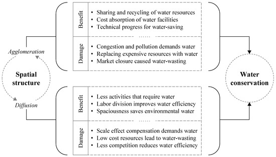
Figure 1.
The theoretical mechanism of spatial structure affecting water conservation.
Furthermore, the drain of resources from cities can have both positive and negative impacts (Figure 1). The most immediate positive consequence is decreased total water use due to fewer social and economic activities. Another potential effect is that cities develop their competitive industries through labor division, thereby increasing water productivity [36]. Furthermore, the cleaner and more spacious environment also saves ecological water utilization [19]. However, the departure of residents and industries may lose the scale effect of production [31]; reduce the price of land, labor, and other resources or goods [34]; and make competition less fierce [35]. These tend to decrease water productivity and even increase water waste.
As discussed above, the development route of the spatial structure that is better for water conservation is uncertain and depends on the development stage of the UA. Resource agglomeration is necessary when the UA has just started to develop. However, the more unbalanced the city development is, the more that negative external costs will be incurred. Thus, the helpfulness of polycentric development on water conservation gradually increases. In fact, most Chinese UAs are in the emerging stage, and their construction was elevated to a national strategic position until 2012 [37]. Even the YRD, the only world-class UA of China, has evident disparities with other peers [38]. Therefore, they are going through a process from agglomeration economy to agglomeration diseconomy. Thus, we hypothesized the following:
Hypothesis 1 (H1).
As the spatial structure moves away from polycentricity, water consumption in the UA will decrease and then increase.
Other factors may be at play when the spatial structure affects water consumption. The population can be an important factor that influences the effect of the spatial structure. In fact, population growth is the most direct manifestation of city expansion [39]. A large city can enjoy the extra benefits of resource agglomeration but incur some environmental and competitive costs. As mentioned earlier, most Chinese UAs are in initial development, so their cities are likely to be located in an agglomeration economy. In this situation, the larger city can enjoy more aggregation benefits and reduce water intensity for cities with different population sizes in the same UA. Thus, the second hypothesis is as follows:
Hypothesis 2 (H2).
In the process of the spatial structure improving water consumption, population plays a reinforcing role.
Another essential factor influencing the effect of the spatial structure can be affluence. Poor cities are often resource-limited, and the initial agglomeration has strong economies of scale. As cities become richer, the infrastructure and market systems gradually improve, and various technologies becomes more advanced. Hence, they may have better ways of developing, and the impact of agglomeration tends to follow general economic laws to show a marginal decreasing trend [34,40]. Clearly, wealthier cities enjoy a lower effect of the spatial structure. Hence, the third hypothesis is proposed:
Hypothesis 3 (H3).
In the process of the spatial structure improving water consumption, affluence plays a weakening role.
3. Materials and Methods
3.1. Model Establishment
The stochastic impacts by regression on population, affluence, and technology (STIRPAT) model, which is derived from the IPAT (Impact, Population, Affluence, and Technology) equation, has been widely used to analyze the influence factors of CO2 emission [41,42,43], energy consumption [44,45,46], and water ecological footprint WEF [47,48,49]. The original version of the STIRPAT model can be expressed as follows:
where denotes the environmental influence, is the population, reflects the affluence, and represents other “technical factors” affecting the environment. For the coefficients, is the constant term, is the error term, and , , and are, respectively, the exponents of , , and . To facilitate estimation and hypothesis testing, the model can be transformed into a linear logarithmic form as follows:
According to the research purpose, actual situations, and the experience of previous studies, we extended the model to consider the spatial-structure index and some other essential variables. Therefore, the extended STIRPAT model can be expressed as follows:
where stands for the WEF, is the spatial structure of UA, and represents the th control variable.
Simultaneously, in order to observe the nonlinear effect of the spatial structure on water consumption, the quadratic term of the spatial-structure index is included as follows:
3.2. Variable Description
3.2.1. Measurement of Water Ecological Footprint
The ecological footprint is an extensively used model that can convert human consumption of various natural resources into the area of land and water. It allows different environmental modification behaviors to be compared under the same framework to analyze the potential for sustainable use of resources in a holistic and precise manner [7]. Therefore, we also convert water consumption into WEF as follows:
where represents the water consumption; stands for the equivalence factor of water resources and is determined to be 5.19, as calculated by the Worldwide Fund for Nature (WWF) [50]; and is the worldwide average production capacity of water, used as 31.4 × 10⁴ m3/km2 [7].
3.2.2. Measurement of Spatial Structure
The rank-size law is a classic and popular method for analyzing the spatial structure of UAs. This law can be traced back to the research of Auerbach [51], who investigated the urban systems of America and Europe and found that the result of multiplying the scale of the urban population and its corresponding rank is approximately a constant, shown as follows:
where stands for the population scale of the city, represents the rank of the city scale, and is the constant term.
The empirical law can be observed in many natural and social domains, such as the distribution of biotic populations, human income, and word frequency. As research has furthered from empirical summarization to theoretical derivation, the rank-size law has been developed into the linear logarithmic form used in this paper, as follows:
where is the coefficient of . Obviously, the value of reflects the steepness of the curve described by the equation.
The larger the value, the steeper the curve, which means the larger the gap between cities and the more concentrated the development of the UA; conversely, the smaller the value, the smaller the gap between cities and the more balanced the development of the UA.
3.2.3. Selection of Control Variables
The control variables are selected as follows: Population () is expressed as the resident population in the urban area. Affluence () is expressed as per capita gross domestic product (GDP). Industrial structure () is measured by the proportion of the tertiary industry in the GDP. Household water intensity () is measured by the water consumption of each water-using population. Productive water intensity () is measured by the water consumption of each added value of the primary and secondary industries. The specific definitions of all variables are summarized in Table 1.

Table 1.
Definition of variables.
3.3. Study Area and Data Sources
3.3.1. Study Area
This study selected the top five national-level UAs identified in the policy document of the outline of the 14th Five-Year Plan (2021–2025) and the Long-range Objectives Through the Year 2035. It specifically includes the JJJ, YRD, PRD, Cheng-Yu urban agglomeration (CY), and urban agglomeration in the middle reaches of the Yangtze River (YRMR). The location of the study area, which covered 92 cities above the prefecture level, is described in Figure 2.
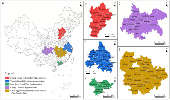
Figure 2.
Location map of top five UAs in China: (a) China, (b) JJJ, (c) YRD, (d) PRD, (e) CY, (f) YRMR.
3.3.2. Data Sources
The data of this study are collected from China Urban Construction Statistical Yearbook, China City Statistical Yearbook, and Statistical yearbooks of some provinces and cities. All price-related data adopt the actual price after eliminating inflation from the base period of 1978. For very few default or abnormal values, we use linear interpolation or the averaging method to fill in the values. Ultimately, balanced panel data consisting of 92 cities from 2006 to 2020 were employed in this study, and the sample descriptive statistics of the main variables are shown in Table 2.
Table 2.
Summary statistics of variables.
4. Results
4.1. Estimates of WEF and Spatial Structure
The WEFs of cities grouped by UAs are shown in Figure 3. From the overall view of the UAs, the total WEF of JJJ shows a trend of first rising and then falling, while other UAs maintain an increasing trend. Furthermore, according to the situation in 2020, the YRD generated the largest WEF of 160.60 thousand km2, followed by PRD with 118.06 thousand km2. YRMR, CY, and JJJ all have a WEF of less than 70 thousand km2. From the internal perspective of each UA, there are often significant gaps between large and small cities, and the major contributions are often made in just a few cities.
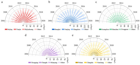
Figure 3.
WEF of top five urban agglomerations in China: (a) JJJ, (b)YRD, (c) PRD, (d) CY, (e) YRMR.
The per capita WEFs of cities grouped by UAs and sorted by annual total WEF from largest to smallest are shown in Figure 4. Cities with a large total WEF tend to have a large per capita WEF, especially in YRD, PRD, and YRMR. Furthermore, many cities in those three UAs have a WEF of more than 2000 m2 per capita, while the WEFs of almost all of the cities in JJJ and PRD are less than 2000 m2. Focusing on the development trend of UAs’ top cities, Shanghai and Wuxi in YRD and almost the entire first third of cities in YRMR have decreased their water intensity, but cities in the other three UAs have barely dropped.
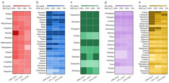
Figure 4.
Per capita WEF of top five UAs in China: (a) JJJ, (b)YRD, (c) PRD, (d) CY, (e) YRMR.
The spatial structures of five UAs are shown in Figure 5. JJJ has the most compact spatial structure but has shown a downward trend in the last five years, from 1.56 in 2016 to 1.32 in 2020. The spatial structures of YRD, PRD, and CY belong to the intermediate level. During the study period, they basically changed between 1 and 1.2 and created a phenomenon of first rising, then falling, and then rising again. Moreover, the YRMR is the most polycentric UA, and it changes from 0.74 in 2006 to 0.83 in 2020. Although there is an upward trend in the YRMR, it has never exceeded 1. In general, the gaps between UAs have narrowed over time, especially the YRD, PRD, and CY, which have become very close in that their standard deviations changed from 0.09 in 2006 to 0.04 in 2020.
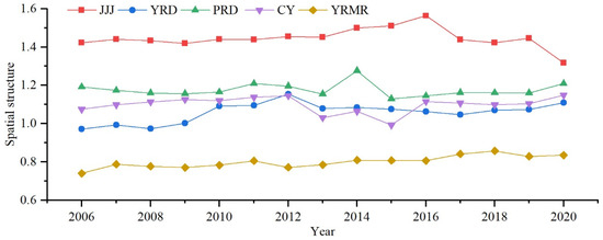
Figure 5.
Spatial structure of top five urban agglomerations in China.
4.2. The General Effect of Spatial Structure on WEF
Firstly, the value of VIF was used to ensure that there were no variables with severe multicollinearity (Table 3). The fixed-effects (FE) model was selected based on the result of the Hausman test to fit the regression equation. Then, in order to alleviate the interference of heteroskedasticity and self-correlation, Driscoll and Kraay standard errors were used to obtain the preliminary estimation result. Furthermore, the endogenous variables of , , and were identified by the Davidson–Mackinnon test. Because of the interaction between these variables and , the one period lagged values for them as instrumental variables (IVs) to regression again by the two-stage least square (2SLS) approach. According to the Kleibergen–Paap rk LM statistic and the Kleibergen–Paap rk Wald F statistic obtained by fitting each regression equation, the validity of the IVs has been proved (Table 4). In addition, a spatial econometric model was also used to consider possible spatial dependencies among the cross sections. Moran’s I, based on the inverse distance spatial weight matrix, is significant at the 1% level but ranges from 0.07 to 0.10, with an average of 0.09. After the tests of LM, Hausman, LR, and Wald, the regression resulting from a Spatial Durbin Model (SDM) with FE was adopted [52,53]. Since Moran’s I is close to 0, and the core explanatory variables did not pass the significance test by the SDM, this paper mainly discusses the regression results of the FE model with IVs.
Table 3.
The VIF value of variables.
Table 4.
Results for general estimation.
The estimation results of Equations (3) and (4) are shown in Table 4. According to the data in column (3), the coefficient of is −1.89, and its -value is less than 0.01. This means that there is sufficient evidence to support the theory that the spatial structure has a negative impact on WEF. Specifically, when other factors remain unchanged, for every 1% increase in the spatial-structure index, the WEF decreases by an average of 1.89%. Moreover, according to the data in column (6), the coefficients of and are −1.86 and 0.91, respectively, which pass the significance test. This illustrates that as the spatial-structure index increases, its influence on WEF decreases and then increases. Hence, Hypothesis 1 is verified.
4.3. Reginal Heterogeneity in the Effect of Spatial Structure
Since China’s five major UAs are at different stages of development, the possible regional heterogeneity is worth further discussion. Considering the fact that the JJJ, YRD, and PRD have more prominent regional advantages in economy, policy, and geographical location, they are classified as first-level UAs, and the other two UAs of CY and YRMR are classified as second-level UAs. Through the addition of interaction terms of category dummy variables, the examination results were obtained and are shown in Table 5. According to the data in column (2), the coefficient of and are −0.59 and 0.58, respectively, which all passed the significance test and are consistent with the direction of the general regression results. Further calculation shows that the inflection point is around 1.03. According to the data in column (3), the coefficients of and are −7.73 and −11.69, respectively, which pass the significance test. This indicates that the cities in second-level UAs are barely past the stage where the spatial-structure index negatively correlates with the WEF.
Table 5.
Results for heterogeneity and regulatory effect.
4.4. Water Account Heterogeneity in the Effect of Spatial Structure
To further investigate whether there is diffidence in the impact of spatial structure on various types of water consumption, two sub-accounts of WEF, namely the household WEF and the productive WEF, were used as the additional explained variables for regressions. The empirical results of the core variables are shown in Table 5. According to the data in column (4), the coefficient of is −0.39, which passes the significance test with a -value less than 0.1, and the coefficient of is −0.42 but is not reliable enough. Moreover, following the data in column (5), the coefficient of is −2.88, which passes the significance test with a -value less than 0.01, and the coefficient of is 0.3469 but is also not reliable enough. Comparing the regression results of the two WEFs, the absolute value of the coefficient of in the productive WEF is much larger than in the household WEF. These values indicate that the water account is heterogeneous in the negative impact of spatial structure. That is, the productive WEF is affected more strongly than the household WEF.
4.5. The Interaction Effect of Spatial Structure and Regulating Indicators on WEF
Considering the regulating role of population and affluence in the process of spatial structure affecting WEF, the interaction of variables of and , as well as the interaction of variables of and are both constructed for regressions. The empirical results are shown in Table 5. According to the data in column (6), the coefficients of and are −1.02 and 1.30, respectively, which pass the significance test and are consistent with the direction of the general regression results. Moreover, the coefficient of is −0.23, which passes the significance test with a -value less than 0.05. This suggests a reinforcing role in the negative impact of spatial structure on WEF, which supports the Hypothesis 2. According to the data in column (7), the coefficients of and are −1.84 and 0.87, respectively, which pass the significance test and are consistent with the direction of the general regression results. Moreover, the coefficient of is 0.14, which does not pass the significance test. Therefore, there is not enough evidence to support the Hypothesis 3.
5. Discussion
Water resources are closely related to human life and production, but China is facing the dilemma of needing to improve residents’ well-being while saving water resources. In the past, China was accustomed to adopting an extensive economic growth pattern [54], resulting in irreparable losses to the ecological environment, including a water resource shortage [7]. Therefore, China has put forward the concept of high-quality development, aiming to move to a path that considers both the environment and the economy [55]. In this strategy, UAs are the critical governance subjects [56]. In the development plan of YRD, which is the most advanced UA in China, the priority of water conservation is clearly emphasized. In addition, many other UA plans contain similar statements.
However, according to the WEF of China’s top five UAs from 2006 to 2020, the task of water conservation is still heavy. Four urban agglomerations have rising total WEFs, and cities with significant contributions almost expand in the same direction as the overall UA, except for Shanghai. As for JJJ, the only UA that has seen a decline in its total WEF, WEFs has declined in it largest city of Beijing, but it has risen in most other cities. In general, water constraints in most cities are becoming tighter. It may be mainly because these cities are still in a period of rapid development [57], and the rise in water consumption is inevitable. More worryingly, many cities with a large total WEF tend to have a large per capita WEF, and there is barely a downward trend in the water intensity. Hence, there needs to be a better way to develop economies with less water intensity.
Then, as a particular property of UA, can the urban spatial structure affect the WEF as it affects energy and air? The results of this study show that water resources can be saved by adjusting the spatial structure. The linear effect of the spatial-structure index on WEF is negative. After adding the quadratic term, it is found that this negative effect will gradually decrease and then turn positive. That is, the impact of spatial-structure index on water consumption can be depicted as a U-shaped curve. According to the regression results for regional heterogeneity, the more developed UAs experience the complete impact characteristic of first falling and then rising, among which only the YRD is located near the inflection point. At the same time, the spatial structure of JJJ and PRD is too centralized. Furthermore, the spatial structure of CY and the YRMR can be more concentrated, which would help to reduce the WEF of their cities. Hence, other solutions may be needed for the cities with a large proportion of household water use. Moreover, according to the estimation of the interaction variable, the population is proven to play a reinforcing role in the process of spatial structure improving WEF. It also reflects the current situation that the agglomeration economy is more significant than the agglomeration diseconomy in most cities. In addition, although the weakening role of affluence has been estimated and is in line with the hypothesis, there is not enough evidence to prove it. This may be because many cities still have much room for economic improvement [57]. Hence, affluence does not obstruct the negative effect of spatial structure on WEF. It can also be considered that, at this stage, the adjustment of the spatial structure can achieve a win-win situation for economic development and water conservation.
6. Conclusions
Based on panel data covering 92 cities in China’s top five agglomerations from 2006 to 2020, the WEF of cities and the spatial structure of the UAs are calculated, and the relationships between them are verified. The following conclusion can be drawn: The water constraints in most cities are becoming tighter. Promoting the balanced development of JJJ and PRD and enhancing the role of the growth pole in CY and YRMR can help water conservation. In addition, by reducing the WEF through agglomeration development, most cities with a large proportion of production WEF or a large population will enjoy more benefits. Conversely, other conventional water-saving policies are needed to compensate for the cities with large shares domestic WEF and small populations.
There are some limitations of the current study, which can serve as a starting point for future research. Firstly, the regulated role of affluence has not obtained enough evidence. Although the results are consistent with the hypothesis, whether affluence can weaken spatial structure’s negative effect on water consumption remains to be confirmed in the future. Secondly, due to data collection difficulties, only the population distribution is used to characterize the spatial structure. If more data are available in the future, more alternative indicators can be adopted to further improve the accuracy of the results. Thirdly, as analyzed in this paper, the spatial structure affects water consumption through some economic and social activities. If there are better methods and data, the specific effect of spatial structure on water consumption can be studied in more detail.
Author Contributions
Conceptualization, Y.L. and C.J.; formal analysis, Y.L. and C.J.; funding acquisition, R.G. and W.Y.; investigation, Y.L., C.J. and J.T.; methodology, R.G.; supervision, R.G. and W.Y.; writing–original draft, Y.L.; writing–review & editing, R.G. All authors have read and agreed to the published version of the manuscript.
Funding
This work was supported by the Philosophy and Social Science Foundation of Hunan Province in China (No. 16YBA166).
Institutional Review Board Statement
Not applicable.
Informed Consent Statement
Not applicable.
Data Availability Statement
The datasets used and analyzed in the research are available from the corresponding author upon request.
Conflicts of Interest
The authors declare no conflict of interest.
References
- Li, F.; Feitelson, E.; Li, Y. Is China at the tipping point? Reconsidering environment-economy nexus. J. Clean. Prod. 2020, 276, 123156. [Google Scholar] [CrossRef]
- Chen, X.; Chen, X.; Song, M. Polycentric agglomeration, market integration and green economic efficiency. Struct. Chang. Econ. Dyn. 2021, 59, 185–197. [Google Scholar] [CrossRef]
- Zhang, L.; Chen, F.; Lei, Y. Climate change and shifts in cropping systems together exacerbate China’s water scarcity. Environ. Res. Lett. 2020, 15, 104060. [Google Scholar] [CrossRef]
- Zeng, P.; Sun, F.; Liu, Y.; Wang, Y.; Li, G.; Che, Y. Mapping future droughts under global warming across China: A combined multi-timescale meteorological drought index and SOM-Kmeans approach. Weather. Clim. Extrem. 2021, 31, 100304. [Google Scholar] [CrossRef]
- Yu, R.; Zhai, P. More frequent and widespread persistent compound drought and heat event observed in China. Sci. Rep. 2020, 10, 14576. [Google Scholar] [CrossRef]
- Xu, X.; Yang, G.; Tan, Y. Identifying ecological red lines in China’s Yangtze River Economic Belt: A regional approach. Ecol. Indic. 2019, 96, 635–646. [Google Scholar] [CrossRef]
- Jin, C.; Liu, Y.; Li, Z.; Gong, R.; Huang, M.; Wen, J. Ecological consequences of China’s regional development strategy: Evidence from water ecological footprint in Yangtze River Economic Belt. Environ. Dev. Sustain. 2022. [Google Scholar] [CrossRef]
- Zhi, Y.; Chen, J.; Qin, T.; Wang, T.; Wang, Z.; Kang, J. Spatial Correlation Network of Water Use in the Yangtze River Delta Urban Agglomeration, China. Front. Environ. Sci. 2022, 10, 924246. [Google Scholar] [CrossRef]
- Huang, Y.; Liao, R. Polycentric or monocentric, which kind of spatial structure is better for promoting the green economy? Evidence from Chinese urban agglomerations. Env. Sci. Pollut. Res. Int. 2021, 28, 57706–57722. [Google Scholar] [CrossRef]
- Zhao, Y.; Wang, Y.; Wang, Y. Comprehensive evaluation and influencing factors of urban agglomeration water resources carrying capacity. J. Clean. Prod. 2021, 288, 125097. [Google Scholar] [CrossRef]
- Babuna, P.; Yang, X.; Bian, D. Water Use Inequality and Efficiency Assessments in the Yangtze River Economic Delta of China. Water 2020, 12, 1709. [Google Scholar] [CrossRef]
- Liu, Y.; Hu, Y.; Su, M.; Meng, F.; Dang, Z.; Lu, G. Multiregional input-output analysis for energy-water nexus: A case study of Pearl River Delta urban agglomeration. J. Clean. Prod. 2020, 262, 121255. [Google Scholar] [CrossRef]
- Dou, P.; Zuo, S.; Ren, Y.; Rodriguez, M.J.; Dai, S. Refined water security assessment for sustainable water management: A case study of 15 key cities in the Yangtze River Delta, China. J. Environ. Manag. 2021, 290, 112588. [Google Scholar] [CrossRef]
- Huang, Z.; Liu, J.; Mei, C.; Wang, H.; Shao, W. Water security evaluation based on comprehensive index in Jing-Jin-Ji district, China. Water Supply 2020, 20, 2698–2714. [Google Scholar] [CrossRef]
- Cai, Y.; Wang, H.; Yue, W.; Xie, Y.; Liang, Q. An integrated approach for reducing spatially coupled water-shortage risks of Beijing-Tianjin-Hebei urban agglomeration in China. J. Hydrol. 2021, 603, 127123. [Google Scholar] [CrossRef]
- Liu, S.; Yang, M.; Mou, Y.; Meng, Y.; Zhou, X.; Peng, C. Effect of Urbanization on Ecosystem Service Values in the Beijing-Tianjin-Hebei Urban Agglomeration of China from 2000 to 2014. Sustainability 2020, 12, 10233. [Google Scholar] [CrossRef]
- Yang, Z.; Xia, J.; Zou, L.; Qiao, Y.; Xiao, S.; Dong, Y.; Liu, C. Efficiency and driving force assessment of an integrated urban water use and wastewater treatment system: Evidence from spatial panel data of the urban agglomeration on the middle reaches of the Yangtze River. Sci. Total Environ. 2022, 805, 150232. [Google Scholar] [CrossRef]
- Yi, H.; Yang, Y.; Zhou, C. The Impact of Collaboration Network on Water Resource Governance Performance: Evidence from China’s Yangtze River Delta Region. Int. J. Environ. Res. Public Health 2021, 18, 2557. [Google Scholar] [CrossRef]
- Yu, B. Urban spatial structure and total-factor energy efficiency in Chinese provinces. Ecol. Indic. 2021, 126, 107662. [Google Scholar] [CrossRef]
- Sun, B.; Han, S.; Li, W. Effects of the polycentric spatial structures of Chinese city regions on CO2 concentrations. Transp. Res. Part D Transp. Environ. 2020, 82, 102333. [Google Scholar] [CrossRef]
- Zhu, K.; Tu, M.; Li, Y. Did Polycentric and Compact Structure Reduce Carbon Emissions? A Spatial Panel Data Analysis of 286 Chinese Cities from 2002 to 2019. Land 2022, 11, 185. [Google Scholar] [CrossRef]
- Wang, M.; Zhang, B. Examining the impact of polycentric urban form on air pollution: Evidence from China. Environ. Sci. Pollut. Res. Int. 2020, 27, 43359–43371. [Google Scholar]
- Li, W.; Sun, B.; Zhang, T.; Zhang, Z. Panacea, placebo or pathogen? An evaluation of the integrated performance of polycentric urban structures in the Chinese prefectural city-regions. Cities 2022, 125, 103624. [Google Scholar] [CrossRef]
- Chen, X.; Zhang, S.; Ruan, S. Polycentric structure and carbon dioxide emissions: Empirical analysis from provincial data in China. J. Clean. Prod. 2021, 278, 123411. [Google Scholar] [CrossRef]
- Williamson, J.G. Regional inequality and the process of national development. Econ. Dev. Cult. Chang. 1965, 13, 1–84. [Google Scholar] [CrossRef]
- Glaeser, E.L.; Resseger, M.G. The complementarity between cities and skills. J. Reg. Sci. 2010, 50, 221–224. [Google Scholar] [CrossRef]
- Han, J.; Li, G.; Shen, Z.; Song, M.; Zhao, X. Manufacturing transfer and environmental efficiency: Evidence from the spatial agglomeration of manufacturing in China. J. Environ. Manag. 2022, 314, 115039. [Google Scholar] [CrossRef]
- Fujita, M.; Thisse, J.F. Economics of agglomeration. J. Jpn. Int. Econ. 1996, 10, 339–378. [Google Scholar] [CrossRef]
- Xu, H.; Jiao, M. City size, industrial structure and urbanization quality—A case study of the Yangtze River Delta urban agglomeration in China. Land Use Policy 2021, 111, 105735. [Google Scholar] [CrossRef]
- Büttner, T.; Schwager, R.; Stegarescu, D. Agglomeration, Population Size, and the Cost of Providing Public Services: An Empirical Analysis for German States. ZEW-Cent. Eur. Econ. Res. Discuss. Pap. 2004, 04–018. Available online: https://www.econstor.eu/bitstream/10419/24041/1/dp0418.pdf (accessed on 20 September 2022).
- Chertow, M.R.; Ashton, W.S.; Espinosa, J.C. Industrial Symbiosis in Puerto Rico: Environmentally Related Agglomeration Economies. Reg. Stud. 2008, 42, 1299–1312. [Google Scholar] [CrossRef]
- Kim, E.; Lee, H. Spatial integration of urban water services and economies of scale. Rev. Urban Reg. Dev. Stud. 1998, 10, 3–18. [Google Scholar] [CrossRef]
- Bottasso, A.; Conti, M. Scale economies, technology and technical change in the water industry: Evidence from the English water only sector. Reg. Sci. Urban Econ. 2009, 39, 138–147. [Google Scholar] [CrossRef]
- Yan, S.; Wang, J. Does Polycentric Development Improve Green Utilization Efficiency of Urban Land? An Empirical Study Based on Panel Threshold Model Approach. Land 2022, 11, 124. [Google Scholar] [CrossRef]
- Liu, J.; Cheng, Z.; Zhang, H. Does industrial agglomeration promote the increase of energy efficiency in China? J. Clean. Prod. 2017, 164, 30–37. [Google Scholar] [CrossRef]
- Xu, C.; Bin, Q.; Shaoqin, S. Polycentric spatial structure and energy efficiency: Evidence from China’s provincial panel data. Energy Policy 2021, 149, 112012. [Google Scholar] [CrossRef]
- Fang, C. Important progress and future direction of studies on China’s urban agglomerations. J. Geogr. Sci. 2015, 25, 1003–1024. [Google Scholar] [CrossRef]
- Tian, Y. Mutualistic Pattern of Intra-Urban Agglomeration and Impact Analysis: A Case Study of 11 Urban Agglomerations of Mainland China. ISPRS Int. J. Geo-Inf. 2020, 9, 565. [Google Scholar] [CrossRef]
- Wei, C.; Taubenböck, H.; Blaschke, T. Measuring urban agglomeration using a city-scale dasymetric population map: A study in the Pearl River Delta, China. Habitat Int. 2017, 59, 32–43. [Google Scholar] [CrossRef]
- Castells-Quintana, D. Malthus living in a slum: Urban concentration, infrastructure and economic growth. J. Urban Econ. 2017, 98, 158–173. [Google Scholar] [CrossRef]
- Zhang, S.; Zhao, T. Identifying major influencing factors of CO2 emissions in China: Regional disparities analysis based on STIRPAT model from 1996 to 2015. Atmos. Environ. 2019, 207, 136–147. [Google Scholar] [CrossRef]
- Lin, S.; Wang, S.; Marinova, D.; Zhao, D.; Hong, J. Impacts of urbanization and real economic development on CO2 emissions in non-high income countries: Empirical research based on the extended STIRPAT model. J. Clean. Prod. 2017, 166, 952–966. [Google Scholar] [CrossRef]
- Wu, R.; Wang, J.; Wang, S.; Feng, K. The drivers of declining CO2 emissions trends in developed nations using an extended STIRPAT model: A historical and prospective analysis. Renew. Sustain. Energy Rev. 2021, 149, 111328. [Google Scholar] [CrossRef]
- Shahbaz, M.; Chaudhary, A.R.; Ozturk, I. Does urbanization cause increasing energy demand in Pakistan? Empirical evidence from STIRPAT model. Energy 2017, 122, 83–93. [Google Scholar] [CrossRef]
- Ji, X.; Chen, B. Assessing the energy-saving effect of urbanization in China based on stochastic impacts by regression on population, affluence and technology (STIRPAT) model. J. Clean. Prod. 2017, 163, S306–S314. [Google Scholar] [CrossRef]
- Xue, L.; Li, H.; Xu, C.; Zhao, X.; Zheng, Z.; Li, Y.; Liu, W. Impacts of industrial structure adjustment, upgrade and coordination on energy efficiency: Empirical research based on the extended STIRPAT model. Energy Strategy Rev. 2022, 43, 100911. [Google Scholar] [CrossRef]
- Xu, M.; Li, C. Influencing factors analysis of water footprint based on the extended STIRPAT model. In Application of the Water Footprint: Water Stress Analysis and Allocation; Springer: Singapore, 2020; pp. 105–126. [Google Scholar]
- Jin, C.; Huang, K.; Yu, Y.; Zhang, Y. Analysis of Influencing Factors of Water Footprint Based on the STIRPAT Model: Evidence from the Beijing Agricultural Sector. Water 2016, 8, 513. [Google Scholar] [CrossRef]
- Zhao, C.; Chen, B.; Hayat, T.; Alsaedi, A.; Ahmad, B. Driving force analysis of water footprint change based on extended STIRPAT model: Evidence from the Chinese agricultural sector. Ecol. Indic. 2014, 47, 43–49. [Google Scholar] [CrossRef]
- Dai, D.; Sun, M.; Xu, X.; Lei, K. Assessment of the water resource carrying capacity based on the ecological footprint: A case study in Zhangjiakou City, North China. Environ. Sci. Pollut. Res. Int. 2019, 26, 11000–11011. [Google Scholar] [CrossRef]
- Auerbach, F. Das gesetz der bevölkerungskonzentration. Petermanns Geogr. Mitt. 1913, 59, 74–76. [Google Scholar]
- Elhorst, J.P. Specification and Estimation of Spatial Panel Data Models. Int. Reg. Sci. Rev. 2003, 26, 244–268. [Google Scholar] [CrossRef]
- Baltagi, B.H.; Liu, L. Testing for random effects and spatial lag dependence in panel data models. Stat. Probab. Lett. 2008, 78, 3304–3306. [Google Scholar] [CrossRef]
- Hu, Y.; Jiang, H.; Zhong, Z. Impact of green credit on industrial structure in China: Theoretical mechanism and empirical analysis. Environ. Sci. Pollut. Res. Int. 2020, 27, 10506–10519. [Google Scholar] [CrossRef] [PubMed]
- Chen, Y.; Tian, W.; Zhou, Q.; Shi, T. Spatiotemporal and driving forces of Ecological Carrying Capacity for high-quality development of 286 cities in China. J. Clean. Prod. 2021, 293, 126186. [Google Scholar] [CrossRef]
- Ma, J.; Wang, J.; Szmedra, P. Economic Efficiency and Its Influencing Factors on Urban Agglomeration—An Analysis Based on China’s Top 10 Urban Agglomerations. Sustainability 2019, 11, 5380. [Google Scholar] [CrossRef]
- Shen, J.; Chen, C.; Yang, M.; Zhang, K. City Size, Population Concentration and Productivity: Evidence from China. China World Econ. 2019, 27, 110–131. [Google Scholar] [CrossRef]


Publisher’s Note: MDPI stays neutral with regard to jurisdictional claims in published maps and institutional affiliations. |
© 2022 by the authors. Licensee MDPI, Basel, Switzerland. This article is an open access article distributed under the terms and conditions of the Creative Commons Attribution (CC BY) license (https://creativecommons.org/licenses/by/4.0/).