Abstract
Harnessing renewable and clean energy resources from winds and tides are promising technologies to alter the high level of consumption of traditional energy resources because of their great global potential. In this regard, developing farms with multiple energy converters is of great interest due to the skyrocketing demand for sustainable energy resources. However, the numerical simulation of these farms during the planning phase might pose challenges, the most significant of which is the computational cost. One of the most well-known approaches to resolve this concern is to use the virtual blade model (VBM). VBM is the implementation of the blade element model (BEM). This was done by coupling the blade element momentum theory equations to simulate rotor operation with the Reynolds averaged Navier–Stokes (RANS) equation to simulate rotor wake and the turbulent flow field around it. The exclusion of the actual geometry of blades enables a lower computational cost. Additionally, due to simplifications in the meshing procedure, VBM is easier to set up than the models that consider the actual geometry of blades. One of the main unaddressed limitations of the VBM code is the constraint of modeling up to 10 renewable energy converters within one computational domain. This paper provides a detailed and well-documented general methodology to develop a virtual blade model for the simulation of 10-plus converters within one computational domain to remove the limitation of this widely used and robust code. The extended code is validated for both the single- and multi-converter scenarios. It is strongly believed that the technical contribution of this paper, combined with the current advancement of available computational resources and hardware, can open the gates to simulate farms with any desired number of wind or tidal energy converters, and, accordingly, secure the sustainability and feasibility of clean energies.
1. Introduction
In response to a growing focus on sustainable development and reducing emissions, renewable energy has come into focus. This approach is encouraged and supported by green funds and climate change action [1]. This energy can be derived from a variety of resources, including solar, wind, ocean, biomass, geothermal, hydroelectric, and hydrogen. Wind energy and tidal stream energy, among others, are estimated to have annual global energy potentials of 875 PWh and 1.2 PWh, respectively [2,3]. Different designs for wind and tidal stream devices have been developed in order to harness this significant potential. In particular, horizontal axis wind turbines (HAWT) and horizontal axis tidal turbines (HATT) have received much attention. Several energy farms have been built at either a small- or commercial scale. It is noteworthy that the levelized costs of electricity for onshore wind and tidal energies are 0.039 and 0.20 USD/kWh, respectively [3,4]. Hence, the high costs of harnessing these types of renewable energies necessitate the numerical modeling of their interactions inside energy farms in order to ensure the optimal layout and reliable operation.
There are several numerical models for wind and tidal turbines, including the sliding mesh model (SMM), rotating reference frame (RRF), virtual blade model (VBM), actuator disc model (ADM), and momentum sink model (MSM). SMM and RRF are near-field models with the highest level of fidelity. The first simulates a rotating turbine using a sliding mesh interface, while the latter simulates the flow field around turbine blades in a reference frame that rotates at the speed of the turbine rotor [5,6]. VBM is an implementation of the blade element model (BEM) within ANSYS FLUENT [7]. In VBM, the actual blades are not directly present and, therefore, eliminates the need for a high-resolution mesh around the turbine blades [5,8]. The ADM represents the turbine as a momentum sink and energy [5]. In ADM, the turbine rotor is modeled as an infinitely thin porous disc [6]. Cross comparisons between the numerical models are provided in Table 1. MSM is a low-fidelity far-field model that is best suited to modeling large arrays of turbines [6]. The MSM simulates the mechanics of energy extraction by momentum sinks in the momentum equations [6]. A detailed comparative analysis of the numerical techniques used for wind and tidal turbines is provided in [5,9], and [6,10], respectively.

Table 1.
Comparison of different modeling approaches for horizontal axis wind and tidal devices [5,6,9,10].
As can be seen in Table 1, the VBM has a very acceptable capability in modeling the performance, wake, and turbulence of wind and tidal turbines and provides good predictions with significantly lower computational costs. Investigations on HAWTs have shown that the lack of physical blade geometry in VBM reduces the meshing time and computational cost by between 10 and 100 times [5,9,10] and therefore, VBM is easier to set up than the models that consider the actual geometry of blades, such as SMM or MRF. To sum up, the critical benefit of VBM is its optimal trade-off of computational cost and wake characterization [11]. Previous studies [5,7] have shown that it can provide appropriate and realistic wake predictions only at a distance of two radii downstream of a turbine. These advantages demonstrate the remarkable capabilities of VBM compared to the blade-resolved methods, making it a viable and efficient tool for interactions between multiple turbines in energy farms (e.g., wind and tidal arrays).
Renewable energy utilization targets will require large-scale farms with multiple devices. So, a computationally cheap tool plays a vital role in developing such energy farms. However, the current version of the VBM code can only model up to 10 rotor zones within one computational domain. Hence, modifying the VBM original code for the simulation of 10-plus rotor zones to remove its limitations is believed to have a remarkable contribution to the existing literature. This is where the novelty of this work lies. For the first time, this paper presents a step-by-step and well-documented methodology for increasing the maximum number of rotors within the VBM code, allowing these codes to simulate the wind or tidal farms with any number of devices.
To achieve this goal, the paper is structured as follows: in Section 2, a comprehensive overview and classification of relevant studies is conducted. Section 3 discusses the concepts and governing equations of the VBM. A step-by-step methodology to modify the original VBM codes is provided in Section 4. In Section 5, we validate the extended VBM codes. Finally, the discussion and potential future research directions are provided in Section 6.
2. Literature Review
2.1. Studies Using VBM
VBM is widely used to model helicopter blades, wind, and tidal energy. A search in SCOPUS and Google Scholar for publications utilizing VBM for numerical simulation of aircraft and wind/tidal turbines returns a total of 41 articles or conference papers released between 2009 and 2021. Figure 1 presents the number of documents per year. Moreover, as can be seen, most of the papers were published in 2018. A closer look at Figure 1 shows that 10 of these studies investigated HAWTs and nine investigated HATTs. Most of which were published in 2017. Nevertheless, it should be noted that there are several theses, dissertations, and reports that used VBM to study HAWTs and HATTs, e.g., [7,12,13,14,15,16,17,18,19]. They are not accounted for in the statistics of the current section.
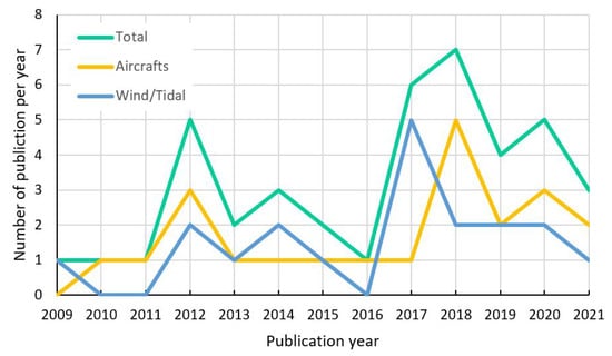
Figure 1.
Number of publications that used VBM for numerical simulation.
VBM was originally developed to numerically simulate the performance and turbulent flow field around helicopter rotors. However, later, it was adapted to simulate single and arrays of horizontal axis wind and tidal turbines. Publications on aircrafts cover the impacts of rotating blades using VBM in different types of aircrafts, including helicopters ([20,21,22,23,24,25,26,27,28,29,30]), unmanned aerial vehicles ([31,32,33]), quad-copters ([34]), turboprops ([35]), and tilt-rotors ([36]). Of these, the helicopter is the most analyzed vehicle (about 60% of all). Additionally, the number of rotors in these studies ranges from one to four.
The classification of studies on HAWTs/HATTs is provided in Table 2. Studies in the table are presented chronologically, from oldest to most recent. As can be seen, a large body of research describes the wake characteristics of HAWTs and HATTs. Chick and Makridis [37] studied the wake interactions of two wind turbines at the top of an ideal Gaussian hill. They found that velocity deficits are higher in the flat terrain cases. Nevertheless, after 10D downstream, the maximum velocity deficit increases in complex cases because of the slowing wind speed. Hussein and El-Shishiny [38] investigated onshore micro-scale wind farms consisting of two HAWTs. Makridis and Chick [39] explored the interaction of wind turbine wakes with the terrain. They examined velocity and turbulence at four downstream locations and identified that the maximum wake deficit overprediction was 15% at 4D. Javaherchi et al. [5] simulated the flow field around and in the wake of a HAWT. They compared three models for HAWT performance and wake characterization, including RRF, VBM, and ADM. Balduzzi et al. [40,41] adapted VBM to analyze the rooftop siting of a wind turbine in an urban landscape. Their results showed that a wrong positioning of a HAWT can result in more than 50% performance losses.
Javaherchi et al. [42,43,44] studied the flow field and energy extraction in a small array of marine hydrokinetic (MHK) turbines (also referred to as HATT). They found that VBM has limitations in modeling the turbine performance accurately at very low and high tip speed ratios (TSRs). Nevertheless, it provides a good compromise between cost and accuracy in rather far wake regions. They also employed the same methodology to investigate sediment transport in wake [45]. Sufian et al. [46,47] developed models to simulate the interaction of a HATT and free surface waves. They concluded that this interaction extended wavelength by about 12% and reduced the wave height by about 10%. Later, Ref. [8] investigated this effect and reported a reduction of 3% in wave height for a single turbine. Their results suggest a 7% increase in bed stress upstream of the turbine.
Bowman et al. [48] proposed a physics-based actuator disk model (PBADM) for a HATT and compared it with ADM and VBM. They reported that VBM over-predicts the wake deficit. Additionally, it produces the most significant amount of transverse velocity. Lombardi et al. [49] explored the effect of blockage and found that the performance of a downstream HATT can increase up to 5% with a lateral spacing of 1.5D. Attene et al. [11] implemented a methodology to maximize tidal stream turbine power. They found that an optimal lateral spacing of 3D between two side turbines in a row increases the turbine power by nearly 20%. Santos et al. [50] studied the wake characteristics and configuration of the HATTs in a river channel and obtained wake lengths between 7 and 9 diameters. Recently, reference [51] adapted VBM to study an array of HATTs and developed a linear methodology to predict the maximum power output of the turbines based on available kinetic energy flux at 1D upstream of HATTs. Reference [52] conducted a literature review on different approaches for wake characterization of hydrokinetic converters, including BEM. They verified that in the simulation of the far wake region, the BEM showed a good balance between accuracy and cost, indicating that it could be used for optimizing turbine spacing in large arrays.
Table 2.
Classification of studies on wind and tidal energy devices using VBM [5,6,10,53].
Table 2.
Classification of studies on wind and tidal energy devices using VBM [5,6,10,53].
| Study | Type | Scope | Objective | Number of Turbines | Turbine Model | Turbine Dimension |
|---|---|---|---|---|---|---|
| [37] | CP | HAWT 1 | Wake interaction | 2 | NREL 5MW | Full |
| [38] | AR | HAWT | Wake interaction | 1, 2 | Tjaereborg turbines | Full |
| [54] | AR | HAWT | Wake interaction | 2 | NTK 500/41 | Full |
| [39] | AR | HAWT | Wakes with terrain effects | 2, 6 | Nibe turbines | Full |
| [42] | AR | HATT | Wake characteristics | 1 | DOE RM1 | Scaled |
| [5] | AR | HAWT | Wake characteristics | 1 | NREL Phase VI | Scaled |
| [46] | CP | HATT 2 | Wake characteristics | 1 | Wortmann FX 63-137 | Scaled |
| [43] | CP | HATT | Wake characteristics | 1 | DOE RM1 | Scaled |
| [53] | AR | HAWT | Wake characteristics | 1 | NREL Phase VI | Scaled |
| [44] | AR | HATT | Wake characteristics | 1 | DOE RM1 | Scaled |
| [47] | AR | HATT | Wave and turbine interaction | 1 | Wortmann FX 63-137 | Scaled |
| [45] | AR | HATT | Sediment transport in wake | 1 | DOE RM1 | Scaled |
| [40] | AR | HAWT | Wake interaction | 1 | NREL Phase II | Scaled |
| [41] | CP | HAWT | Wake interaction | 1 | NREL Phase II | Scaled |
| [48] | AR | HATT | Wake characteristics | 1 | Wortmann FX 63-137 | Scaled |
| [8] | AR | HATT | Wave and turbine interaction | 1 | Hull University model | Scaled |
| [11] | AR | HATT | Wake interaction in tidal array | 1, 2 | IFREMER model | Scaled |
| [49] | AR | HATT | Effect of the blockage | 1, 2 | Wortmann FX 63-137 | Full, Scaled |
| [50] | AR | HATT | Wake characteristics | 1, 3 | Notre Dame turbine | Full |
1 Horizontal Axis Wind Turbine. 2 Horizontal Axis Tidal Turbine.
Articles and conference papers focused on HAWTs and HATTs from 2009 to 2021 are listed in Table 2. They are classified and organized based on the purpose of each study, the number of turbines, turbine model, and turbine dimension. Basically, the VBM methodology was developed and validated for HAWTs and HATTs by taking advantage of the similar underlying physics of these two different engineering technologies. As seen in Table 2, the majority of studies simulated a scaled version of turbine designs and a handful number of turbines. These simulations are not in line with the current significant demand for the study and development of energy farms. An overview of the literature that relates to HATTs found that far-field models (MSM and the bed roughness model (BRM)) are the most common models to investigate the impacts of turbine arrays [6]. As it was concluded from Table 1, they are low-fidelity models unable to capture the near wake characteristics and performance of turbines. This shortage motivates the need for a cost-effective and reliable technique to explore wind and tidal arrays. Hence, VBM would be of great interest in this respect. This necessitates the current study to remove the limitation of 10 rotors in the original codes of VBM. Another important aspect is that “NREL” and “DOE RM1” reference models are the most common benchmark designs for HAWTs and HATTs. Furthermore, almost all studies focused on wake characterization (interaction with other turbines, waves, and water surfaces).
Since, this paper focuses on a farm of tidal stream energy converters to validate its methodology, the next subsection overviews some of the recent literature on the optimization of these farms. See [55] for a comprehensive review on the technologies, design considerations and numerical models of tidal current turbines.
2.2. Tidal Farm Optimization
Although it is widely acceptable that tidal current energy sources can act as key drivers of sustainability, their economic feasibility is questionable in many countries. Therefore, in order to secure sustainable energy resources, it is of paramount importance to develop methodologies to optimize the layout of tidal farms and exploit maximum available clean energy from tidal streams. There are many studies focusing on the different aspects of optimizing tidal stream farms. Among others, Thiébot et al. [56] discussed several approaches for the numerical modeling of hydrodynamics and tidal energy extraction in the Alderney Race (AR), France. They mentioned two aspects of layout optimization: “macro-design” to determine the density of converters according to the possible flow diversion; and “micro-design” to adjust the individual converters’ layout. As summarized in [56], optimization using a gradient-based method using the adjoint method in the software package OpenTidalFarm is an example of macro-design used in the AR. They also highlighted the crucial impact of neglecting flow interactions and weak representation of the wake field in the micro-design process of finding the optimal arrangement. So, there is an urgent need for more advanced computational techniques, such as BEM, to gain more insight into the local processes affecting turbine loading and performance. Additionally, Jung [57] used the gradient-based optimization using the adjoint method to study the effects of unsteady flow on the optimization of a tidal farm in Korea. The gradient-based approach is well known and implemented in several other studies (see [58,59] for the adjoint method, and [60,61] for the swarm optimization algorithm). Genetic algorithms are also deployed for the purpose of tidal farm optimization in the AR (see [62]).
Integrating cost and benefit in the optimization process have also been of interest in the literature. Reference [63] implemented a mixed-integer programming methodology to optimize potential tidal current farms in the Chacao Channel, Chile. They highlighted the accurate characterization of wake effects as an interesting future work to extend their methodology. Reference [64] presented a novel approach for this purpose, involving the design of experiments, computational fluid dynamics simulations (CFD), surrogate model construction, and a combination of geometric, economic and environmental constraints for the optimization. For the CFD model, they employed ADM to represent the flow field. They proposed to incorporate BEM for the better modeling of hydrodynamic loads on rotor blades. As can be seen, the findings of the current research complement previous methodologies by enhancing the modeling capabilities and flexibility of a version of the BEM method implemented in RANS solvers, such as ANSYS FLUENT. It is worth mentioning that deep learning techniques may also be used for this purpose (see, for example, [65,66]), but it is out of the scope of this study.
3. Virtual Blade Model (VBM)
In 1995, Zori et al. [67] published a general computational fluid dynamics (CFD) code that greatly yet efficiently simplified the numerical modeling approach to simulate a helicopter rotor operation and flow field around it. Later on, the implementation of the published code by Zori et al. was adapted within ANSYS FLUENT, significantly enhancing its usage and application [68]. The originality of this code lies under the efficient modeling of the helicopter rotor blade shape, with variable profile shape and angles along the blade span, and their effect on the surrounding flow via the blade element momentum theory (BEMT) equations [69]. The distinction between BEMT and VBM is that the latter incorporates all three components of the RANS momentum equations, while the former uses only a simplified equation [11]. This approach eliminates the requirement of generating, gridding, and numerically simulating the helicopter rotor blade’s complex geometry and flow field and simulating it virtually (i.e., virtual blade model). This exclusion of the actual geometry of blades from the numerical modeling of the turbine blades reduces computational costs even up to 100 times while providing an accurate effect of the turbine far wake and turbine–turbine wake interaction [9,16]. As the actual geometry of blades is not directly present in the model, the name virtual blade model (VBM) is used for this rotor representation [5]. The general idea of VBM is that it models the effect of the rotating turbine blades on its surrounding flow field (i.e., rotor wake) via coupling the solution of BEM equations with the Reynolds averaged Navier–Stokes (RANS) equations. In this respect, the BEM solution is integrated into the RANS equation as an external body force (i.e., through source terms in the momentum equations [39]). This process is done iteratively until a converged numerical solution for the rotor operation in the flow field is attained.
In the VBM, the turbine blade span is divided into small elements from root to tip (up to 20 sections), and the lift and drag forces of sections are computed based on the local angle of attack (AOA), chord length, and airfoil shape. The lift and drag forces for each section are calculated as follows [7]:
where is the chord length of the segment and is provided by the manufacturer, is the fluid density, A is the rotor swept area, is the fluid velocity relative to the blade, and are the lift- and drag coefficients that come from a lookup table that contains the values as a function of the Mach number (Ma), the Reynolds number (Re) and AOA for the blade airfoils. AOA is defined as follows [13]:
where U is the streamwise velocity (i.e., the velocity perpendicular to the plane of rotation), is the angular velocity, and R is the radius of the rotor disk. This rotor disk zone is a thin fluid sub-domain with an area equal to the blades’ swept area over a complete revolution. It should be noted that the dynamic effect of blades rotation is simulated based on the time-averaged body forces over the thin full disk. Accordingly, the lift and drag forces are averaged over a full blade revolution to calculate the forces per cell as follows [14]:
where is the number of blades, r is the radial position of the blade section from the center of the turbine, and is the azimuthal coordinate.
This time-averaged force is used to calculate the equivalent source term for each mesh cell. Therefore, the momentum source term for each cell of the numerical discretization is [14]:
where is the volume of the grid cell. These forces are applied to the fluid at each calculation step, and the flow is updated. This iterative process continues until the convergence is reached [13]. As can be seen, VBM indirectly considers the effect of rotating blades through the introduction of momentum source terms that act within the rotor disk zone [49]. A brief description of general steps to implement VBM within ANSYS FLUENT is provided in Appendix A.
4. Methodology
VBM is a set of four user defined functions (UDFs) developed in C programming language for use in ANSYS FLUENT. Modifications were made to simulate 10-plus rotor zones in the original UDF code written in C language. The four UDFs are as follows:
- rotor_model_v10.1.c;
- rotor_model_v10.scm;
- thread_mem_v1.0.c;
- thread_mem.h.
In the current version of the code, modifications were made to simulate 20 rotor zones. In this regard, the first two UDFs will be updated, and the other two will remain unchanged. Needless to say, it is possible to model infinite rotor zones by employing the present methodology. It is only a matter of understanding where modifications must be made.
4.1. Changes Applied to “rotor_model_v10.1.c”
The core calculations are performed through “rotor_model_v10.1.c”. This UDF consists of four sections: “Global Input Variables”, “Global Trimming Variables”, “Global Memory”, and “All Functions”. The code structure is depicted in Figure 2. Each function has its specific variables and uses some global variables. These global variables play an important role in the calculations of rotor zones and are used by most functions. Therefore, they are introduced at the beginning of all functions.
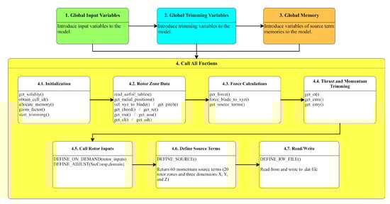
Figure 2.
Structure of the main code and its functions.
The first section deals with the global input variables. The first and foremost variable that is utilized is “nrtz”, which represents the number of rotor zones. The quantity of this variable is introduced via GUI as an integer number. The previous version of the code was limited to 10-rotor zones, and extended to 20-rotor zones. Following nrtz, the code reads settings related to the number of blades, rotor radius, rotor speed, tip effect, rotor disk origin and angle, blade pitch and flapping, number of blade sections, twist and chord specifications, and lift- and drag coefficients. The number of rotor zones directly influences these variables. It means that the number of rotor zones controls how many times a loop should be executed in a function. So they must be changed and extended to 20. It should be noted that some of these arrays may have more than one dimension (e.g., twist and chord specifications, or lift- and drag coefficients: variables cin, cout, csec, twst, and clorcd), but only the dimension which is related to the number of rotor zones must be modified. For most of these variables, it is the first dimension; on the other hand, it is the second or the third for a few of them.
In the next section, trimming variables are provided and should be modified to consider 20 rotor zones. It is worth mentioning that trim variables for the soft-in-plane isotropic blade [70]. Nevertheless, they are not applicable for the simulation of the horizontal axis wind or tidal turbines and remain disabled in the VBM panel. In the global memory section, the number of rotor cell zone and source terms are introduced to the model. These variables are related to nrtz and extended to 20.
In the next step, functions are explored to check their local variables. A few of these functions contain the variables as mentioned above and are related to the number of rotor zones. Therefore, modifications were made to account for 20 rotor zones. The VBM code outputs are momentum source terms that are in three dimensions. A function in the code is responsible for calculating momentum quantities. Another function, executed at the final stage of the code, returns these quantities to ANSYS FLUENT software. In order to make a connection between these two functions, momentum quantities should be stored in the memory. This memory allocation is executed in the first part of section four. Every single rotor zone has a counter and three momentum quantities. In other words, every rotor zone requires four memory allocations. Since the number of rotor zones is doubled, these memory allocations are also modified from 10 to 20 in the next step (lines 237–416 in the original code and 237–488 in the modified code).
For large problems with a massive number of cells, the code must run in parallel mode. For this reason, in some parts, data are transmitted from the host to node processors and vice versa. The number of times the data are transmitted between hosts and nodes is proportional to the number of rotor zones. Consistent with the rest of the modifications, this number is changed from 10 to 20. These modifications are applied to lines 2790–2850 of the original code (lines 2862–2922 of the modified code).
The final part of the code consists of functions that return momentum quantities to the RANS solver (here, ANSYS FLUENT). There are three functions, named “DEFINE_SOURCE”, for a single rotor zone to return momentum sources in all three directions. For these functions, it is required to add X-Y-Z momentum source terms to account for 11 to 20 rotor zones. This is carried out in lines 4199–5018 of the modified code. Other minor modifications are also highlighted in the difference check of the original and extended codes (it is included as the paper’s Supplementary Material). All in all, as a result of the applied changes, the number of lines of the code is increased from 4239 to 5129.
4.2. Changes Applied to “rotor_model_v10.scm”
The function of this file is written in the SCHEME language to enable VBM in the list of available models inside ANSYS FLUENT and input all rotor parameters through a GUI panel. A modification is made to this file. In section “GEOMETRY–Hub–Number of Sections Details” and line 597, ‘maximum 10’ is replaced by ‘maximum 20’. This extends the number of rotor zones from 10 to 20.
5. Results and Discussion
This section outlines the numerical results to validate the developed model. In order to do this, the new VBM codes are used to simulate two case studies with 1 and 12 MHK turbines. It is noteworthy that high-fidelity methods, such as SRF, are not suitable for simulating multiple tidal or wind converters in a farm due to the high computational cost. Hence, they cannot be used to compare with VBM in a tidal farm scenario with more than 10 converters. On the other hand, VBM is a well-known tool for simulating HAWTs and HATTs, and several studies have already discussed its effectiveness in comparison with other available approaches. Therefore, this paper’s aim is not to compare the results of VBM against other techniques, such as SRF and ADF. Readers are referred to [5] for the comparison of SRF, VBM, and ADF for a HAWT model, and [16] for a HATT model.
In view of the above, this section of the paper is arranged so that the results for a single turbine are validated first. DOE reference model 1 (DOE RM1) [71] is used for this purpose since it is a publicly available model for further validation, and the extracted power results for this reference model are available for both SRF and VBM models. Using this comparison, the extended VBM model of the present paper is validated for a single turbine. After that, the extended code is used to simulate a row of 12 tidal converters perpendicular to the surrounding flow. In order to conclude that the developed code works correctly, the output power from all converters should be equal due to the fact that they are all arranged in a row and receive the same amount of incoming flow velocity. However, small discrepancies may occur due to the interaction of adjacent tidal converters. In the following, the results for single and multiple tidal energy converters are presented and discussed.
5.1. Validation of a Single Turbine Model
The results of previous studies in the National Renewable Energy Laboratory (NREL) [71], and Multiphase and Cardiovascular Flow Lab at the University of Washington [72] are used to validate the developed model for a single turbine case. The general settings and adapted numerical schemes are based on the previous study of the authors ([51]) on MHK turbines. In our model, inlet and outlet boundaries are modeled as velocity inlet and pressure outlet, respectively (see Figure 3). At the inlet boundary, the free stream velocity is 1.9 m/s. The turbine hub is modeled as a no-slip wall, and the outer boundaries of the model are slip-free walls. A DOE RM1 is used as a reference model in the present study. This is an open-source design for a horizontal axis hydrokinetic turbine developed in the National Renewable Energy Laboratory (NREL), and researchers can use it to benchmark their studies [71]. This MHK turbine has a diameter (D) of 20 m, and its rotor speed is 11.5 rpm. To specify the turbulence, the turbulence intensity is 5%, and the length scale is 1 m. The turbulence intensity is defined as the ratio of the root-mean-square of the velocity fluctuations to the mean flow velocity [72]. In turbulent flows, the turbulence length scale describes the size of the large eddies that contain most of the energy. Accordingly, the tip speed ratio (TSR) equals 6.3. TSR and is formulated as follows:
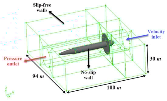
Figure 3.
Sketch of the computational domain for single-converter and boundary conditions.
The blockage ratio is a determinant factor in comparing the amount of power extracted since it indicates how much tidal current passes through blades. It is calculated by dividing the rotor sweep area (A) by the area of the inlet boundary. To ensure reproducibility and comparability, the blockage ratio used in this study should be equal to 11.1% as in the study by Tessier and Tomasini [72]. Since , the area of the velocity inlet should be 2820 m. The depth of the model is assigned 30 m to represent the actual water depth of the pilot farm adapted for validation in Section 5.2. Therefore, the width of the single-converter model for validation purposes is equal to 94 m as demonstrated in Figure 3. Essentially, it is the ratio between the rotor-swept area and the inlet boundary area. It should be mentioned that, as opposed to the two benchmarks, our CFD model captures the real geometry of the turbine hub, while the hub is modeled as a thin porous zone within the two benchmarks. Results are summarized in Table 3. ANSYS FLUENT reports the extracted power for each rotor as an outcome of the VBM model execution. Comparison with benchmark studies on the DOE RM1 model in Table 3 demonstrates the quality of the developed VBM model used in this study. Results indicate that the calculated power of the high fidelity SRF model in [71] is 504 kW, and its difference with our model is ≈, which is very satisfactory and promising.
Table 3.
Power comparison between current model and two benchmark models.
Another important aspect is the efficiency of tidal energy converters. If the efficiency () is defined as the power extracted by the turbine in a specific array position, normalized by the power available in the undisturbed flow at the inlet of the channel,
For the amounts of efficiency for the current study, and the studies by NREL [71] and Tessier and Tomasini [72] are 0.456, 0.415, and 0.448, respectively. It should be noted that according to [69], the maximum theoretical efficiency of tidal converters must respect Betz’s limit on the maximal power that can be extracted and is equal to . Although all of the calculated efficiencies are consistent with Betz’s limit, as stated by [72], the values close to 50% for the efficiency with the current state of development are considered high and most likely not representative of real efficiency values in experiments or the field. So, it can be assumed all these numerical simulations over-predict the real power extracted by the blade.
5.2. Validation for a Tidal Farm Model
This section shows the further validation of the developed model for tidal arrays with 12 turbines (case of 10-plus rotor zones). As discussed earlier, in the present study, the operation of turbines inside a farm is simulated via BEM coupled with RANS. Sketch of the computational domain and imposed boundary conditions are presented in Figure 4. It was decided to use this layout of turbines because the interpretation of the results for the validation of the model would be quite straightforward. If all rows of turbines have the same extracted power, then the developed code is working correctly and will be validated. As seen in Figure 4, the farm has a rectangular cross section, and its dimensions are with a hub-to-hub distance of . The uniform stream-wise velocity at the inlet has a magnitude of 1.75 m/s (this velocity is based on the real tidal stream velocity of the selected farm based on the previous study [73]). The surrounding flow is seawater, and its density is 1025 kg/m. Inlet and outlet boundaries are modeled as the velocity inlet and pressure outlet, respectively. The other walls of the computational domain are modeled as slip-free walls, and as proposed by [42], the turbine nacelle is set as a no-slip condition to capture its effect on wake recovery. The mesh is structured in most of the computational domain except for the regions close to the nacelles. This study’s resolution of mesh needed for a mesh-independent solution is based on the developments in [51]. The user should pay attention to avoid duplicate faces in the meshing of the rotor zone. The mesh must have a full 360-unit circular face as the rotor face.
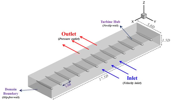
Figure 4.
Sketch of the computational domain for multi-converter configuration and boundary conditions.
In the paper, the RANS simulation is closed with shear stress transport or SST as the turbulent model, where is the turbulence kinetic energy, and the is specific dissipation rate [16]. This model is a modification of the original to overcome its limitations for capturing the turbulent boundary layer around the blade. SST transitions to the model for better far-field characterization. Turbulence equations are set to be a second-order upwind scheme. The semi-implicit method for pressure linked equations (SIMPLE) algorithm is deployed as a pressure-velocity scheme to solve the RANS equations. Additionally, the discretizations of gradient, pressure and momentum for modeling the flow field around turbine blades are “Green-Gauss Node Based”, “Second-Order”, and “QUICK”.
Figure 5 illustrates the results obtained using the modified VBM codes and the above-mentioned numerical settings. They represent the velocity contours in the y-direction of a single-row tidal farm with 12 MHK turbines. The velocities are normalized according to the stream-wise velocity at the inlet ( m/s). The smooth stream-wise velocity contours in this figure support that the model is fully converged. Additionally, as shown in Figure 5, the flow accelerates around the blades and between turbine nacelles, and as a result, the flow velocity increases to . It should be noted that this accelerated flow affects the sedimentation process and is environmentally essential. There is a significant velocity deficit behind the blades (or rotor swept area) because of the extraction of power. Table 4 summarizes the calculated powers of turbines. The results indicate that the total power extracted from this turbine’s configuration is 5316 kW. The most significant observation of this validation test is that there is a negligible difference () between the calculated powers of the 12 rotors. As it should be, the extracted powers are almost similar and equal to 443 kW. With these results, it is well confirmed that the modified code works correctly for 10 to 20 rotors and the developed methodology can be used reliably to extend the VBM codes and model any desired number of turbines.
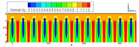
Figure 5.
Velocity contours in the y-direction for a single row tidal farm with 12 active rotors.
Table 4.
Calculated powers of a single row tidal farm with 12 active rotors.
Regarding the efficiency, the s of tidal energy converters within this farm can be estimated as
Following the discussions of the Betz’s limit in Section 5.1, it must be clarified again that although this does not violate the maximum theoretical efficiency, reaching efficiencies close to 50% is idealistic and is a sign of overestimation in such numerical models. This aspect of numerical simulation of tidal energy converters is worthy of further investigation in future studies.
6. Conclusions
The sustainability and feasibility of renewable energy resources necessitate the development of farms with an optimal amount of exploited clean energy. In this regard, the current study aimed at proposing a methodology to modify UDFs of the virtual blade model (VBM), which is an implementation of BEM within RANS solver (here, ANSYS FLUENT). A good wake and performance representation of VBM, as it provides cost effectiveness, makes it a very attractive approach to be used in the numerical investigation of wind and tidal turbine arrays. A step-by-step methodology is provided to update the source codes of VBM and enable it to consider 10-plus rotor zones. DOE reference model 1 (DOE RM1) [71], which is an open-source design, was used to validate the single-rotor model. The power output from the extended VBM code was compared against two benchmark results by [71] for the SRF model, and by [72] for the VBM model. The results show that our computational model for a single-rotor underestimates the corresponding results from the SRF model only by ≈, which is remarkable. Then, the validity and applicability of the modified code shown for a single-row array with 12 MHK turbines (of the type DOE RM1) were arranged in a row to validate the performance of our extended model in a multi-rotor scenario. Our findings indicated that the extracted powers of all the converters are almost similar and equal to 443 kW, with a negligible difference of . This finding is expected since the tidal energy converters are all arranged in a row and receive the same amount of incoming flow velocity. Therefore, it can be concluded that the extended VBM code works properly, and we successfully validated it for both single- and multi-rotor scenarios. In addition, the total power extracted from this turbines’ configuration in our pilot tidal farm is 5316 kW.
Overall, the proposed approach can be generalized to any desired number of turbines. It is strongly believed that this detailed and well-documented general methodology would be a significant step toward the reliable and efficient modeling of wind and tidal farms. Further investigation can be undertaken to explore the performance the extended VBM code in real sites with varying bed profile and flow velocities. As stated in the introduction, wind energy is a greater global energy source and has a lower levelized cost of energy than tidal energy. In addition, wind farms have been built on a large scale around the world. Hence, it will be of great interest to compare the numerical simulation of a wind farm with the field results using the developed code. Finally, a potential future research direction is to deploy it to study wind and tidal farms with tens of turbines and compare the results with low fidelity far-field models, such as MSM or BRM.
Supplementary Materials
The following supporting information can be available at: https://bitbucket.org/vbm-develop/modified-vbm/src/master/ (accessed on 20 October 2022).
Author Contributions
Conceptualization, S.R., M.N., M.M.N. and B.K.; Methodology, S.R.; Software, B.K. and S.R.; Validation, S.R.; Formal analysis, B.K. and S.R.; Investigation, S.R., M.N. and B.K.; Resources, S.R.; Data curation, S.R.; Writing—original draft preparation, S.R. and B.K.; Review and editing, M.N. and M.M.N.; Visualization, S.R.; Supervision, S.R. and M.N.; Correspondence, S.R. All authors have read and agreed to the published version of the manuscript.
Funding
This research received no external funding.
Data Availability Statement
The new developed VBM codes that support the findings of this study are available at https://bitbucket.org/vbm-develop/modified-vbm/src/master/ (accessed on 20 October 2022), or upon request from the Corresponding author.
Acknowledgments
Authors gratefully acknowledge Amir Teymour Javaherchi Mozafari for his help and guidance to set up VBM in ANSYS FLUENT.
Conflicts of Interest
The authors declare no conflict of interest.
Abbreviations
The following abbreviations are used in this manuscript:
| A | Rotor swept area |
| ADM | Actuator disc model |
| AOA | Angle of attack |
| BEM | Blade element model |
| BEMT | Blade element momentum theory |
| BRM | Bed roughness model |
| Lift- and drag coefficients | |
| Chord length for each segment of the blade | |
| Lift and drag forces for each segment of the blade | |
| HATT | Horizontal axis tidal turbines |
| HAWT | Horizontal axis wind turbines |
| Mach number | |
| MHK | Marine hydrokinetic |
| MSM | Momentum sink model |
| Number of blades | |
| NREL | National Renewable Energy Laboratory |
| R | Radius of the rotor disk |
| RANS | Reynolds averaged Navier–Stokes |
| r | Radial position of the blade section from the center of the turbine |
| Reynolds number | |
| RRF | Rotating reference frame |
| SIMPLE | Semi-implicit method for pressure linked equations |
| SMM | Sliding mesh model |
| Azimuthal coordinate | |
| TSR | Tip speed ratio |
| U | Streamwise velocity |
| UDF | User-defined function |
| Volume of the grid cell | |
| Fluid velocity relative to the blade | |
| VBM | Virtual blade model |
| Angular velocity |
Appendix A. General Steps to Implement VBM inside ANSYS FLUENT
This section provides a brief description of VBM model setup within ANSYS FLUENT. General steps to setup the VBM model are as follows:
- 1.
- Setup model: According to the physics of the flow field, the user will select the required models to simulate the flow. As mentioned earlier, VBM averages the effect of rotating blades and as a result, in the vast majority of problems it should be run in steady mode. For unsteady implementation, the model UDF should be modified accordingly. In this step, the user downloads the two sources script files “rotor_model_v11.c” and thread_mem_v1.0.c along with the header file thread_mem.h, and then build and load them within ANSYS FLUENT to enable and compile the VBM model. Then, the geometry of rotor (number of sections, radius, chord length and twist degree) is defined, and the model is set up completely.
- 2.
- Set up working fluid and solids: The user will provide the physical and thermodynamical properties of the working fluid, such as air or water, and solids in the problem via the VBM panel. The momentum sources in X, Y and Z directions for each rotor are defined in this step.
- 3.
- Setup boundary and zone conditions: Solving the governing equations of the flow (i.e., system of partial differential equations) requires well-defined boundary conditions within the CFD domain. These conditions are selected and defined in this step.
- 4.
- Setup solution methods: In CFD simulations, the governing equations of the flow are solved numerically. Based on the physics of the problem, appropriate “pressure-velocity scheme” and “discretization method for gradient, pressure, momentum and turbulent viscosity” are selected at this step.
The modified VBM codes that support the findings of this study are available at https://bitbucket.org/vbm-develop/modified-vbm/src/master/ (accessed on 20 October 2022). For more helpful resources about the implementation of VBM, visit the SFO project by Dr. Amir Teymour Javaherchi Mozafari at https://nbviewer.org/github/sfo-project/3D-flow-over-WindTidal-turbine-VBM-turbulent/blob/master/Fluent/README.ipynb (accessed on 20 October 2022).
References
- Filom, S.; Radfar, S.; Panahi, R.; Amini, E.; Neshat, M. Exploring wind energy potential as a driver of sustainable development in the southern coasts of iran: The importance of wind speed statistical distribution model. Sustainability 2021, 13, 7702. [Google Scholar] [CrossRef]
- Eurek, K.; Sullivan, P.; Gleason, M.; Hettinger, D.; Heimiller, D.; Lopez, A. An improved global wind resource estimate for integrated assessment models. Energy Econ. 2017, 64, 552–567. [Google Scholar] [CrossRef]
- IRENA. Innovation Outlook: Ocean Energy Technologies; Technical Report; International Renewable Energy Agency: Abu Dhabi, United Arab Emirates, 2020. [Google Scholar]
- IRENA. Future of Wind: Deployment, Investment, Technology, Grid Integration and Socio-Economic Aspects (A Global Energy Transformation Paper); Technical Report; International Renewable Energy Agency: Abu Dhabi, United Arab Emirates, 2019. [Google Scholar]
- Javaherchi, T.; Antheaume, S.; Aliseda, A. Hierarchical methodology for the numerical simulation of the flow field around and in the wake of horizontal axis wind turbines: Rotating reference frame, blade element method and actuator disk model. Wind Eng. 2014, 38, 181–201. [Google Scholar] [CrossRef]
- Nash, S.; Phoenix, A. A review of the current understanding of the hydro-environmental impacts of energy removal by tidal turbines. Renew. Sustain. Energy Rev. 2017, 80, 648–662. [Google Scholar] [CrossRef]
- Mozafari, A.J. Numerical Modeling of Tidal Turbines: Methodology Development and Potential Physical Environmental Effects. Master’s Thesis, University of Washington, Seattle, WA, USA, 2010. [Google Scholar]
- Li, X.; Li, M.; Jordan, L.B.; McLelland, S.; Parsons, D.R.; Amoudry, L.O.; Song, Q.; Comerford, L. Modelling impacts of tidal stream turbines on surface waves. Renew. Energy 2019, 130, 725–734. [Google Scholar] [CrossRef]
- Bianchini, A.; Balduzzi, F.; Gentiluomo, D.; Ferrara, G.; Ferrari, L. Comparative analysis of different numerical techniques to analyze the wake of a wind turbine. In Proceedings of the Turbo Expo: Power for Land, Sea, and Air; ASME Digital Collection; American Society of Mechanical Engineers: New York, NY, USA, 2017; Volume 50961, p. V009T49A017. [Google Scholar]
- Masters, I.; Williams, A.; Croft, T.N.; Togneri, M.; Edmunds, M.; Zangiabadi, E.; Fairley, I.; Karunarathna, H. A comparison of numerical modelling techniques for tidal stream turbine analysis. Energies 2015, 8, 7833–7853. [Google Scholar] [CrossRef]
- Attene, F.; Balduzzi, F.; Bianchini, A.; Campobasso, M.S. Using Experimentally Validated Navier-Stokes CFD to Minimize Tidal Stream Turbine Power Losses Due to Wake/Turbine Interactions. Sustainability 2020, 12, 8768. [Google Scholar] [CrossRef]
- Gosset, A.; Flouriot, G. Optimization of Power Extraction in an Array of Marine Hydrokinetic Turbines; Technical Report; French Naval Academy: Lanvéoc, France, 2008. [Google Scholar]
- Cerisola, A. Numerical Analysis of Tidal Turbines Using Virtual Blade Model and Single Rotating Reference Frame; Department of Mechanical Engineering, University of Washington: Seattle, WA, USA, 2012. [Google Scholar]
- Chen, Z. Analyzing Wind Turbine Wakes with Virtual Blade Model Technology Using Openfoam. Ph.D. Thesis, Texas Tech University, Lubbock, TX, USA, 2013. [Google Scholar]
- Adamski, S.J. Numerical Modeling of the Effects of a Free Surface on the Operating Characteristics of Marine Hydrokinetic Turbines. Ph.D. Thesis, University of Washington, Seattle, WA, USA, 2013. [Google Scholar]
- Javaherchi Mozafari, A.T. Numerical Investigation of Marine Hydrokinetic Turbines: Methodology Development for Single Turbine and Small Array Simulation, and Application to Flume and Full-Scale Reference Models. Ph.D. Thesis, University of Washington, Seattle, WA, USA, 2014. [Google Scholar]
- Hoseyni Chime, A. Analysis of Hydrokinetic Turbines in Open Channel Flows. Ph.D. Thesis, University of Washington, Seattle, WA, USA, 2014. [Google Scholar]
- Li, X. Three-Dimensional Modelling of Tidal Stream Energy Extraction for Impact Assessment. Ph.D. Thesis, The University of Liverpool, Liverpool, UK, 2016. [Google Scholar]
- Sufian, S.F. Numerical Modelling of Impacts from Horizontal Axis Tidal Turbines. Ph.D. Thesis, The University of Liverpool, Liverpool, UK, 2016. [Google Scholar]
- McAlpine, J.D.; Koracin, D.R.; Boyle, D.P.; Gillies, J.A.; McDonald, E.V. Development of a rotorcraft dust-emission parameterization using a CFD model. Environ. Fluid Mech. 2010, 10, 691–710. [Google Scholar] [CrossRef]
- Pandey, K.; Kumar, U.; Kumar, G.; Deka, D.; Das, D.; Surana, A. CFD Analysis of an Isolated Main Helicopter Rotor for a Hovering Flight at Varying RPM. In Proceedings of the ASME International Mechanical Engineering Congress and Exposition, Houston, TX, USA, 9–15 November 2012; Volume 45172, pp. 543–551. [Google Scholar]
- Stalewski, W.; Żółtak, J. Optimisation of the helicopter fuselage with simulation of main and tail rotor influence. In Proceedings of the ICAS Congress, Brisbane, Australia, 23–28 September 2012. [Google Scholar]
- Bernardo, P.; Mac Réamoinn, R.; Cardiff, P.; Keenahan, J.; Young, P. CFD Modelling of Helicopter Downwash and Assessment of its impact on Pedestrian Comfort. In Proceedings of the 2018 Civil Engineering Research in Ireland Conference (CERI 2018), University College Dublin, Dublin, Ireland, 29–30 August 2018. [Google Scholar]
- Stalewski, W. Simulation and optimization of control of selected phases of gyroplane flight. Computation 2018, 6, 16. [Google Scholar] [CrossRef]
- Żółtak, J. Multi-objective and multi-disciplinary design using evolutionary methods applied to aerospace design problems. Proc. Inst. Mech. Eng. Part G J. Aerosp. Eng. 2018, 232, 613–625. [Google Scholar] [CrossRef]
- Kusyumov, A.; Kusyumov, S.; Mikhailov, S.; Romanova, E.; Phayzullin, K.; Lopatin, E.; Barakos, G. Main rotor-body action for virtual blades model. In Proceedings of the EPJ Web of Conferences, Frascati, Italy, 26–28 October 2018; Volume 180, p. 02050. [Google Scholar]
- Bernardo, P.; Réamoinn, R.M.; Young, P.; Brennan, D.; Cardiff, P.; Keenahan, J. Investigation of the helicopter downwash effect on pedestrian comfort using CFD. Infrastruct. Asset Manag. 2019, 8, 133–140. [Google Scholar] [CrossRef]
- Stajuda, M.; Obidowski, D.; Karczewski, M.; Jóźwik, K. Modified virtual blade method for propeller modelling. Mech. Mech. Eng. 2020, 22, 603–618. [Google Scholar] [CrossRef]
- Stalewski, W.; Surmacz, K. Investigations of the vortex ring state on a helicopter main rotor using the URANS solver. Aircr. Eng. Aerosp. Technol. 2020, 92, 9. [Google Scholar] [CrossRef]
- Linton, D.; Widjaja, R.; Thornber, B. Actuator Surface Model with Computational-Fluid-Dynamics-Convected Wake Model for Rotorcraft Applications. AIAA J. 2021, 59, 8. [Google Scholar] [CrossRef]
- Hosseini, Z.; Ramirez-Serrano, A.; Martinuzzi, R.J. Ground/wall effects on a tilting ducted fan. Int. J. Micro Air Veh. 2011, 3, 119–141. [Google Scholar] [CrossRef]
- Tran, D.K.K.; Nguyen, K.; Le, T.H.H.; Nguyen, N.H. Numerical Simulation for The Forward Flight of the Tri-copter Using Virtual Blade Model. J. Adv. Res. Fluid Mech. Therm. Sci. 2020, 67, 1–32. [Google Scholar]
- Wang, C.H.J.; Nathanael, J.C.; Ng, E.M.; Ng, B.F.; Low, K.H. Framework for the Estimation of Safe Wake Separation Distance between Same-Track Multi-Rotor UAS. In Proceedings of the AIAA Scitech 2021 Forum, Virtual Event, 11–15 and 19–21 January 2021; p. 0708. [Google Scholar]
- Imam, A.; Bicker, R. Effects of propeller blade twist on reconnaissance quad-rotor UAV. In Proceedings of the International Conference on Applied Mechanics and Mechanical Engineering, Hongkong, China, 3–4 August 2012; Volume 15, pp. 1–15. [Google Scholar]
- Ruiz-Calavera, L.; Funes-Sebastian, D.; Perdones-Diaz, D. Powered model wind tunnel tests of a high-offset subsonic turboprop air intake. In Proceedings of the 46th AIAA/ASME/SAE/ASEE Joint Propulsion Conference & Exhibit, Nashville, TN, USA, 25–28 July 2010; p. 6502. [Google Scholar]
- Li, P.; Zhao, Q.; Zhu, Q. CFD calculations on the unsteady aerodynamic characteristics of a tilt-rotor in a conversion mode. Chin. J. Aeronaut. 2015, 28, 1593–1605. [Google Scholar] [CrossRef]
- Chick, J.; Makridis, A. CFD Modeling of the Wake Interactions of Two Wind Turbines on a Gaussian Hill. In CFD Modeling of the Wake Interactions of Two Wind Turbines on a Gaussian Hill; Firenze University Press: Florence, Italy, 2009; pp. 1000–1004. [Google Scholar]
- Hussein, A.S.; El-Shishiny, H.E. Modeling and simulation of micro-scale wind farms using high performance computing. Int. J. Comput. Methods 2012, 9, 1240025. [Google Scholar] [CrossRef]
- Makridis, A.; Chick, J. Validation of a CFD model of wind turbine wakes with terrain effects. J. Wind Eng. Ind. Aerodyn. 2013, 123, 12–29. [Google Scholar] [CrossRef]
- Balduzzi, F.; Bianchini, A.; Gentiluomo, D.; Ferrara, G.; Ferrari, L. Rooftop siting of a small wind turbine using a hybrid BEM-CFD model. In Research and Innovation on Wind Energy on Exploitation in Urban Environment Colloquium; Springer: New York, NY, USA, 2017; pp. 91–112. [Google Scholar]
- Balduzzi, F.; Bigalli, S.; Bianchini, A. A hybrid BEM-CFD model for effective numerical siting analyses of wind turbines in the urban environment. J. Phys. Conf. Ser. 2018, 1037, 072029. [Google Scholar] [CrossRef]
- Javaherchi, T.; Stelzenmuller, N.; Seydel, J.; Aliseda, A. Experimental and numerical analysis of a scale–model horizontal axis hydrokinetic turbine. In Proceedings of the 2nd Marine Energy Technology Symposium, Seattle, WA, USA, 15–18 April 2014. [Google Scholar]
- Javaherchi, T.; Stelzenmuller, N.; Aliseda, A. Experimental and numerical analysis of a small array of 45: 1 scale horizontal axis hydrokinetic turbines based on the DOE reference model. In Proceedings of the 3rd Marine Energy Technology Symposium, Washington, DC, USA, 27–29 April 2015; Volume 27. [Google Scholar]
- Javaherchi, T.; Stelzenmuller, N.; Aliseda, A. Experimental and numerical analysis of the performance and wake of a scale–model horizontal axis marine hydrokinetic turbine. J. Renew. Sustain. Energy 2017, 9, 044504. [Google Scholar] [CrossRef]
- Javaherchi, T.; Aliseda, A. The transport of suspended sediment in the wake of a marine hydrokinetic turbine: Simulations via a validated Discrete Random Walk (DRW) model. Ocean Eng. 2017, 129, 529–537. [Google Scholar] [CrossRef][Green Version]
- Sufian, S.F.; Li, M. 3D-CFD Numerical Modeling of Impacts From Horizontal Axis Tidal Turbines in The Near Region. Coast. Eng. Proc. 2014, 1, 30. [Google Scholar] [CrossRef]
- Sufian, S.F.; Li, M.; O’Connor, B.A. 3D modelling of impacts from waves on tidal turbine wake characteristics and energy output. Renew. Energy 2017, 114, 308–322. [Google Scholar] [CrossRef]
- Bowman, J.; Bhushan, S.; Thompson, D.S.; O’Doherty, D.; O’Doherty, T.; Mason-Jones, A. A Physics-Based Actuator Disk Model for Hydrokinetic Turbines. In Proceedings of the 2018 Fluid Dynamics Conference, Atlanta, GA, USA, 25–29 June 2018; p. 3227. [Google Scholar]
- Lombardi, N.; Ordonez-Sanchez, S.; Zanforlin, S.; Johnstone, C. A hybrid BEM-CFD virtual blade model to predict interactions between tidal stream turbines under wave conditions. J. Mar. Sci. Eng. 2020, 8, 969. [Google Scholar] [CrossRef]
- dos Santos, I.F.S.; Camacho, R.G.R.; Tiago Filho, G.L. Study of the wake characteristics and turbines configuration of a hydrokinetic farm in an Amazonian river using experimental data and CFD tools. J. Clean. Prod. 2021, 299, 126881. [Google Scholar] [CrossRef]
- Radfar, S.; Panahi, R.; Nezhad, M.M.; Neshat, M. A Numerical methodology to predict the maximum power output of tidal stream arrays. Sustainability 2022, 14, 1664. [Google Scholar] [CrossRef]
- Nago, V.G.; dos Santos, I.F.S.; Gbedjinou, M.J.; Mensah, J.H.R.; Tiago Filho, G.L.; Camacho, R.G.R.; Barros, R.M. A literature review on wake dissipation length of hydrokinetic turbines as a guide for turbine array configuration. Ocean Eng. 2022, 259, 111863. [Google Scholar] [CrossRef]
- Bianchini, A.; Balduzzi, F.; Gentiluomo, D.; Ferrara, G.; Ferrari, L. Potential of the Virtual Blade Model in the analysis of wind turbine wakes using wind tunnel blind tests. Energy Procedia 2017, 126, 573–580. [Google Scholar] [CrossRef]
- Chen, Z.X.; Marathe, N.; Parameswaran, S. CFD Study of Wake Interaction of Two Wind Turbines. Adv. Mater. Res. 2012, 472, 2726–2730. [Google Scholar] [CrossRef]
- Nachtane, M.; Tarfaoui, M.; Goda, I.; Rouway, M. A review on the technologies, design considerations and numerical models of tidal current turbines. Renew. Energy 2020, 157, 1274–1288. [Google Scholar] [CrossRef]
- Thiébot, J.; Coles, D.; Bennis, A.C.; Guillou, N.; Neill, S.; Guillou, S.; Piggott, M. Numerical modelling of hydrodynamics and tidal energy extraction in the Alderney Race: A review. Philos. Trans. R. Soc. A 2020, 378, 20190498. [Google Scholar] [CrossRef] [PubMed]
- Jung Won, J. Effects of Unsteady Flow on the Tidal Turbine Farm Layout Optimization. Ph.D. Thesis, Seoul National University, Seoul, Korea, 2022. [Google Scholar]
- Funke, S.W.; Farrell, P.E.; Piggott, M. Tidal turbine array optimisation using the adjoint approach. Renew. Energy 2014, 63, 658–673. [Google Scholar] [CrossRef]
- Han, J.; Jung, J.; Hwang, J.H. Optimal configuration of a tidal current turbine farm in a shallow channel. Ocean Eng. 2021, 220, 108395. [Google Scholar] [CrossRef]
- Noel, M.M. A new gradient based particle swarm optimization algorithm for accurate computation of global minimum. Appl. Soft Comput. 2012, 12, 353–359. [Google Scholar] [CrossRef]
- Tao, S.; Xu, Q.; Feijóo-Lorenzo, A.E.; Zheng, G.; Zhou, J. Optimal layout of a Co-Located wind/tidal current farm considering forbidden zones. Energy 2021, 228, 120570. [Google Scholar] [CrossRef]
- Fakhri, E.; Thiébot, J.; Gualous, H.; Machmoum, M.; Bourguet, S. Overall tidal farm optimal design—Application to the alderney race and the fromveur strait (France). Appl. Ocean Res. 2021, 106, 102444. [Google Scholar] [CrossRef]
- Aguayo, M.M.; Fierro, P.E.; Rodrigo, A.; Sepúlveda, I.A.; Figueroa, D.M. A mixed-integer programming methodology to design tidal current farms integrating both cost and benefits: A case study in the Chacao Channel, Chile. Appl. Energy 2021, 294, 116980. [Google Scholar] [CrossRef]
- González-Gorbeña, E.; Qassim, R.Y.; Rosman, P.C. Multi-dimensional optimisation of Tidal Energy Converters array layouts considering geometric, economic and environmental constraints. Renew. Energy 2018, 116, 647–658. [Google Scholar] [CrossRef]
- Abualigah, L.; Zitar, R.A.; Almotairi, K.H.; Hussein, A.M.; Abd Elaziz, M.; Nikoo, M.R.; Gandomi, A.H. Wind, solar, and photovoltaic renewable energy systems with and without energy storage optimization: A survey of advanced machine learning and deep learning techniques. Energies 2022, 15, 578. [Google Scholar] [CrossRef]
- Fujiwara, R.; Fukuhara, R.; Ebiko, T.; Miyatake, M. Forecasting design values of tidal/ocean power generator in the strait with unidirectional flow by deep learning. Intell. Syst. Appl. 2022, 14, 200067. [Google Scholar] [CrossRef]
- Zori, L.A.; Rajagopalan, R.G. Navier—Stokes Calculations of Rotor—Airframe Interaction in Forward Flight. J. Am. Helicopter Soc. 1995, 40, 57–67. [Google Scholar] [CrossRef]
- Ruith, M. Unstructured, multiplex rotor source model with thrust and moment trimming-Fluent’s VBM model. In Proceedings of the 23rd AIAA Applied Aerodynamics Conference, Toronto, ON, Canada, 6–9 June 2005; p. 5217. [Google Scholar]
- Burton, T.; Jenkins, N.; Sharpe, D.; Bossanyi, E. Wind Energy Handbook; John Wiley & Sons: Hoboken, NJ, USA, 2011. [Google Scholar]
- Yuan, K.; Friedmann, P.P. Aeroelasticity and Structural Optimization of Composite Helicopter Rotor Blades with Swept Tips; Technical Report; NASA: Washington, DC, USA, 1995. [Google Scholar]
- Lawson, M.J.; Li, Y.; Sale, D.C. Development and verification of a computational fluid dynamics model of a horizontal-axis tidal current turbine. In Proceedings of the International Conference on Offshore Mechanics and Arctic Engineering, Rotterdam, The Netherlands, 19–24 June 2011; Volume 44373, pp. 711–720. [Google Scholar]
- Tessier, M.; Tomasini, N. Numerical Study of Horizontal Axis Hydrokinetic Turbines: Performance Analysis and Array Optimization; Technical Report; Department of Mechanical Engineering, University of Washington: Seattle, WA, USA, 2010. [Google Scholar]
- Radfar, S.; Panahi, R.; Javaherchi, T.; Filom, S.; Mazyaki, A.R. A comprehensive insight into tidal stream energy farms in Iran. Renew. Sustain. Energy Rev. 2017, 79, 323–338. [Google Scholar] [CrossRef]


Publisher’s Note: MDPI stays neutral with regard to jurisdictional claims in published maps and institutional affiliations. |
© 2022 by the authors. Licensee MDPI, Basel, Switzerland. This article is an open access article distributed under the terms and conditions of the Creative Commons Attribution (CC BY) license (https://creativecommons.org/licenses/by/4.0/).