The Impact of Urbanization Level on Urban–Rural Income Gap in China Based on Spatial Econometric Model

Abstract

With the rapid development of China’s economy, urbanization is gradually accelerating, but the income gap between urban and rural areas is growing, which may constrain economic development. To test the impact of urbanization on the urban–rural income gap, this paper uses panel data of 31 provinces (cities/autonomous regions) in China from 2007 to 2018, and combines ArcGIS technology to construct Spatial Dubin Model. This paper finds that the increase in urbanization level in China can significantly reduce the urban–rural income gap. The mediating effects model further shows that the increased level of urbanization in China promotes the flow of factors, which helps the flow of capital and advanced technology into the countryside and increases productivity. It also promotes the transfer of a large amount of surplus labor to the tertiary sector, adjusting the industrial structure and increasing the income of peasants moving to the city. In addition, the development of urbanization in China can lead to the construction of public education, improving the conditions and quality of education and teaching, and increasing the possibilities for farmers to earn high incomes. As a result, the urban–rural income gap in China has been narrowed. The findings of this paper are useful for understanding the underlying mechanisms in the level of urbanization and the urban–rural income gap in China. It provides policy insights for accelerating China’s new urbanization process and promoting the coordinated development of China’s urban and rural regions.

1. Introduction

In recent years, with the rapid development of China’s economy, the position of Chinese cities in globalization has been strengthened [1]. Chinese cities have not only made achievements in traditional manufacturing, but also performed well in producer services, such as high-tech and financial industries. The economic influence of Chinese cities is growing in the world [2], and major Chinese cities have gradually become important command and control centers of the global economy [2,3]. However, the income gap between the rich and the poor has become increasingly prominent, especially the income inequality between urban and rural residents, which has become the main manifestation of China’s income gap [4,5,6,7]. According to the data from the research group on the income distribution of Chinese residents, Luo et al. (2020) [4] found that the Gini coefficient of resident income increased from 0.381 in 1988 to 0.49 in 2007, far exceeding the income inequality threshold of 0.4 set by the United Nations Development Programme (UNDP). Moreover, the 19th session of the National Congress of the Communist Party of China noted that the principal social contradiction has transformed into the contradiction between people’s increasing demands for a better life and unbalanced and inadequate development [8] (http://www.gov.cn/zhuanti/cpcnc/19da/mobile/huizhong.htm, accessed on 12 January 2020). These findings illustrate that the income equity issues have grown to become a significant roadblock to the sound and sustainable development of China’s economy [4].

The Chinese government at all levels has formulated a series of agricultural policies with the goal of increasing farmers’ income and reducing the urban–rural income gap through secondary distribution, including increasing farmers’ transfer payments and rural investment and offering farmers preferential subsidies [9,10]. However, years of policy implementation reveal that while these policies have somewhat narrowed the growing urban–rural income gap, the relative poverty in rural areas has not yet decreased significantly [10,11,12]. The urban–rural income gap remains wide. Therefore, the Chinese government aims to break the traditional dual urban—rural economic structure, transfer the rural surplus labor force, and increase farmers’ income by accelerating the urbanization process [12]. The transfer of rural labor force to cities and towns, on the one hand, can help improve the urban labor supply, boost competition in the urban labor market, and lower the wages of the urban labor force; on the other hand, it can decrease the rural surplus labor force and raise labor productivity and income levels in rural areas, thereby reducing the urban–rural income gap [13].

In fact, a large number of studies show that urbanization is conducive to narrowing the urban–rural income gap [14,15,16,17,18]. Liu (2014) conducted an empirical test by constructing a fixed effects model based on the evidence of Chinese enterprises, and found that urbanization promoted the accumulation of human capital and increased income, thereby reducing the income gap [19]. Glaeser and Lu (2018) conducted an empirical test using data from the Chinese Household Income Project (CHIP) and found that urbanization promoted the free flow of population, increased income and employment opportunities, and finally reduced the urban–rural income gap [20].

However, notably, some studies believe that with the progress of urbanization, the urban–rural income gap will exhibit a U-shaped trend of decreasing and then rising [21,22,23]. This is because the development strategy of giving priority to heavy industries implemented in Chinese cities has limited cities’ ability to absorb labor, which has sacrificed a large number of employment opportunities and put great pressure on urban employment. In order to protect urban residents’ job opportunities, the urban-biased policy was implemented to limit the opportunity and scope of peasant households to obtain positions in cities through administrative or economic means [24]. More importantly, the implementation of China’s household registration system has led to “household registration discrimination” in the process of urbanization, which has increased the urban–rural income gap [25]. Based on an empirical test using provincial panel data between 1996 and 2015, Hong et al. (2021) found that government-driven urbanization has led to an improvement in China’s urbanization level with no economic growth [26]. In particular, the effectiveness of urbanization policies in narrowing the urban–rural income gap will be limited by regional economic development and cultural disparities. By comparing the data on China’s population migration in 2005 and 2015, Hus and Ma (2021) found that the urban–rural income gap narrowed faster in cities with looser household management [25]. Moreover, “household registration discrimination” led to a 15.6% reduction in farmers’ income.

The above research serves as a good reference for identifying the relationship between urbanization and the urban–rural income gap, but there are common limitations in these studies. The utilization of timeseries data and the panel data model in the aforementioned studies does not take the spatial dependence and spillover effect of urbanization and urban–rural income into account, which will lead to errors in the model specification and bias in the empirical test results [22]. A reasonable explanation is that because of the serious disparity in economic development between Chinese provinces, there are huge differences in market development between different provinces. Take the Beijing–Tianjin–Hebei region as an example; in addition to a direct local impact, Beijing’s urbanization strategy will have a spillover effect on the strategies of Tianjin, Hebei, and other provinces and cities.

Based on this, this paper uses a spatial econometric model to quantitatively test the relationship between urbanization level and urban–rural income gap on the basis of verifying the spatial correlation of the provincial income gap. The results of empirical tests show that the improvement of urbanization level significantly reduces the urban–rural income gap, and there is a spatial spillover effect of this impact. The improvement of urbanization level in this region helps to reduce the urban–rural income gap in adjacent areas. The results of further mechanism tests show that the improvement of urbanization level will affect the urban–rural income gap through human capital accumulation, industrial structure optimization and technology improvement.

Therefore, unlike previous studies that focus on the impact of urbanization on urban–rural income in one region, this study analyzes the spatial agglomeration pattern of urbanization in various provinces and cities in the Chinese mainland, which is also the main innovation of this paper. Specifically, to solve the problem of the bias caused by ignoring the influence of spatial autocorrelation and ensure the consistency of the estimation results, this paper introduces the spatial effect of urbanization on urban–rural income gap into the quantitative model. Additionally, given that the spatial relationship can deepen the analysis of the internal impact mechanism between urbanization and the urban–rural income gap, this paper can provide a decision basis and policy suggestions for promoting the layout of new urbanization, which has strong theoretical and practical significance.

2. Literature Review

Overall, China’s economy has continued to grow rapidly over a long period of time, but at the same time, it has amassed a number of contradictions that result from uneven development, which have aggravated the problem of income inequality. More and more scholars are starting to pay attention to the urban–rural income gap and identify factors including age, gender, and educational background as potential causes. Moreover, with the growing prominence of the dual urban—rural economic structure in China, scholars have begun to focus on how external factors such as urbanization affect the urban–rural income gap.

2.1. Research on the Influence of Urbanization Factors on the Urban–Rural Income Gap

Against the background of ongoing urbanization in China, some scholars deem that urbanization can facilitate the movement of capital, technology, human resources, and other elements, while maximizing its externality. Urbanization can promote the equalization of human capital, educational level, technical level, and other factor payments, optimize resource allocation by increasing efficiency, raise market dynamics, and realize a virtuous cycle, thereby narrowing the urban–rural income gap [7,26]. At the same time, the optimization of human capital and educational level in rural areas is beneficial to improving the quality of labor and further expanding their opportunities to obtain high income [26]. Additionally, a large quantity of returned high-quality labor, and their social capital and advanced technologies, will promote the production scale and mechanization in rural areas or the incubation of new local industries, such as agritainment, ecotourism, Internet + Agriculture, etc., which will increase the expected return [20,27,28]. Based on an empirical test using the cross-sectional data of 1995, 2002, and 2007, as well as firm-level data, Guo et al. (2022) found that urbanization has significantly narrowed the urban–rural income gap [11]. The main reason is that urbanization provides farmers with fairer employment opportunities and improves their income. Sheng et al. (2022) conducted an empirical test using the data of five agricultural surveys from 2000 to 2018, and found that the advancement of urbanization in China led to an increase of 47 million to 71 million in non-agricultural employment, which significantly reduced the urban–rural income gap [29].

However, some scholars deem that there are “negative effects” in the process of urbanization. The dualistic structural system of urban and rural areas that originated from the household registration system restricts the migration and flow of population between urban and rural areas. Moreover, the poorer groups are in a vulnerable position in the aspects of factor acquisition, identification, utilization, and reprocessing, which increases the possibility of the wealthy rural residents becoming city dwellers through economic means [30,31]. A large number of rural labor forces have made great contributions to urban construction, but they cannot equally enjoy the development dividends brought by urbanization, such as public services, educational resources, employment opportunities, and social security, and their children may even face more serious schooling barriers. All of these have led to a more serious intergenerational problem of education gaps, and increased the uncertainty of migrant workers’ income, thus widening the urban–rural income gap [30,32]. Through an empirical test using the instrumental variable method and the data of Chinese representative families in 2013, Liao and Zhang (2021) found that the peasant migrants’ incomes are about 20% lower than those of urban households. The main reason is that rural household registrations bring more uncertainty to the migrant population, including limited access to loans and education [31]. Wu and Zheng (2018) demonstrated that the household registration system will widen the urban–rural income gap by constructing counterfactuals through the propensity score matching method and the double difference method, based on the data of two Chinese general social surveys (CGSS) [1].

Additionally, some scholars deem that the impact of urbanization on the urban–rural income gap is uncertain, which should be determined according to the level of the income gap [33,34,35]. A small number of people with high capital and technology in rural areas took the lead in entering the urban industrial sector, which increased the urban–rural income gap. Subsequently, more rural populations have migrated to cities, which has gradually narrowed the income gap within rural areas [4,8,36]. Zhong et al. (2022) constructed a model for empirical testing using the data of 220 prefecture-level cities in China from 2006 to 2014, and found that in the early stage of urbanization, every 1% increase in urban land would lead to a 0.011% reduction in the urban–rural income gap [12]. However, when the urbanization rate exceeds 50%, there is a negative correlation between urban sprawl and the urban–rural income gap, characterized by an inverted U-shaped relationship between the urbanization rate and the urban–rural income gap. Based on the Ordinary Least Squares (OLS) model using the panel data of 29 provinces in China from 1978 to 2008, with the time trend controlled, Chen and Lin (2013) confirmed that the urban–rural income gap in China presents a U-shaped curve in the process of urbanization, and the prior development of heavy industry has led to the expansion of the urban–rural income gap in China [33]. In order to solve the endogeneity problem, they selected the logarithm of “distance from threats”, which refers to the shortest distance from each provincial capital city to the northern boundary line, the eastern coastline, or the southern coastline, as the instrumental variable to further confirm the above results.

2.2. Other Correlative Factors Affecting the Urban–Rural Income Gap

Firstly, economic factors have an impact on the urban–rural income gap. The urban–rural income gap exhibits various trends in different stages of economic growth. The income gap among people fluctuates from low to high, then back to low, as the economy develops from the initial stage to the rising stage and to the mature stage [34,35,36]. For instance, Luo (2012) discussed how economic growth may narrow or expand the income gap according to Datt–Ravallion and Shapley decomposition [37]. A typical example is that the economic growth between 2002 and 2007 led to the welfare of the poor being impaired. At the same time, expanding the rural financial scale will widen the urban–rural income gap, but improving rural financial efficiency is conducive to narrowing the urban–rural income gap [8].

Secondly, institutional factors have an important impact on the urban–rural income gap. The long-term urban-biased policy has formed a dualistic structural system of urban and rural areas, which restricts the free flow of labor and distorts the urban–rural factor prices. Moreover, this system has encouraged wealthier rural residents to become urban residents first, which further widens the urban–rural income gap [4,8]. For instance, due to the current household registration system based on the dualistic structure system of urban and rural areas, rural residents frequently experience household registration discrimination in job hunting, which reduces their income by 3.5% on the whole. Furthermore, due to the long-term barrier between rural and urban areas caused by China’s household registration system, moving to the city is exceedingly expensive for rural residents [38,39]. Assuming that there is no household registration discrimination, the Gini coefficient will be significantly reduced, and the overall household consumption will be improved [12]. Rural residents’ lack of equal right to education, as well as income inequality caused by the difference in human capital level, will in turn limit the opportunities of low-income people to improve their human capital, such as receiving education and training, which will further reduce the human capital of low-income people and widen the urban–rural income gap [27,38,39]. In conclusion, the large difference in urban–rural human capital, the distortion of the supply–demand relationship in the labor market, and the unidirectional flow of rural labor into cities have all led to the continuous expansion of the urban–rural income gap in China.

Thirdly, scholars have also studied the impact of social factors on the urban–rural income gap, in addition to the economic and institutional factors. Based on the specific analysis, Han and Kong (2020) found that regardless of whether the manufacturing industry emigrates or transfers, the labor flow will expand the urban–rural income gap [40,41]. The agglomeration of producer services can not only directly narrow the urban–rural income gap in China, but also have an indirect negative impact on income inequality by promoting urbanization and human capital accumulation [11,19]. Additionally, according to other scholars, the improvement of public infrastructure is conducive to narrowing the urban–rural income gap [18,28,42]. The main reason is that the improvement of public infrastructure can not only reduce information asymmetry, optimize resource allocation between urban and rural areas, and attract more labor, but it can also indirectly narrow the urban–rural income gap by improving the quality of human capital and technology [8,18]. Therefore, with the advancement of urbanization and the improvement of human capital level, the income redistribution effect of public infrastructure is gradually enhanced.

2.3. Literature Analysis

The relationship between urbanization and the urban–rural income gap has been the subject of extensive scholarly research, which serves as a source of inspiration and reference for the theoretical framework and model specification in this paper. However, the existing research still has the following deficiencies.

Firstly, previous studies have ignored the spatial dependence and spillover effects of urbanization and the urban–rural income gap. Time series and panel data have been utilized in the current research to build fixed effects, Gaussian Mixed Model, double differences, and other models to identify the relationship between urbanization and the urban–rural income gap. However, these studies did not consider the spatial dependence and spillover effect of urbanization and the urban–rural income gap, so their model specification and the corresponding estimation results are biased. Chinese provinces are characterized by unevenness due to their differences in economic development, institutional environment, and market power, and are closely connected at the same time to the exchange of needed goods, especially in the Yangtze River Delta, the Beijing–Tianjin–Hebei region, the Pearl River Delta, and the Chengdu-Chongqing Economic Circle. Therefore, this paper studies the relationship between urbanization and the urban–rural income gap from the perspective of spatial spillover effects using the provincial panel data from 2007 to 2018. Moreover, from the perspective of spatial spillover effects using the provincial panel data from 2007 to 2018, this paper performs a quantitative test on the relationship between urbanization and the urban–rural income gap by solving the problem of the bias caused by ignoring the influence of spatial autocorrelation, which ensures the consistency of the estimation results.

Secondly, existing mechanisms do not take into account the impact of spatial factors. When analyzing the internal influence mechanism between urbanization and the urban–rural income gap, the existing literature often neglects the impact of spatial factors on the estimation results, leading to inconsistent conclusions being reached by different scholars. Therefore, in order to reasonably explain this inconsistency, this paper incorporates the spatial spillover effect into the model to quantitatively investigate the internal influence mechanism.

3. Model Specification and Estimation Method

3.1. Model Specification

On the basis of analyzing whether the research object has spatial spillover effects through $\mathrm{Moran}$ test and local indicators of spatial association (LISA) images, this paper constructs a spatial econometric model to quantitatively test the spatial effect of urbanization on the urban–rural income gap.

3.1.1. Spatial Autocorrelation

The premise of building a spatial econometric model is to determine whether the research object has spatial autocorrelation, which can be distinguished by the spatial autocorrelation coefficient $\mathrm{Global} \mathrm{Moran}\prime \mathrm{s} \mathrm{I}$. Referring to the method of Jiang et al., (2022) [18], $\mathrm{Moran}\prime \mathrm{s} \mathrm{I}$ can be calculated by the following formula:

$$\mathrm{Moran}\prime \mathrm{I}=\frac{{\sum }_{\mathrm{i}=1}^{\mathrm{n}}{\sum }_{\mathrm{j}=1}^{\mathrm{n}}{\mathrm{W}}_{\mathrm{ij}}\left({\mathrm{Y}}_{\mathrm{i}}-\overline{\mathrm{Y}}\right)({\mathrm{Y}}_{\mathrm{j}}-\overline{\mathrm{Y}})}{{\mathrm{S}}^2{\sum }_{\mathrm{i}}^{\mathrm{n}}{\sum }_{\mathrm{j}}^{\mathrm{n}}{\mathrm{W}}_{\mathrm{ij}}}$$

(1)

where ${\mathrm{S}}^2=\sum _{\mathrm{i}=1}^{\mathrm{n}} {({\mathrm{Y}}_{\mathrm{i}}-\overline{\mathrm{Y}})}^2/\mathrm{n}$, and ${\mathrm{W}}_{\mathrm{ij}}$ is a 0–1 spatial weight matrix. The value range of $\mathrm{Moran}\prime \mathrm{s} \mathrm{I}$ is (−1, 1). A value lager than 0 indicates a positive spatial autocorrelation between regions; a value less than 0 indicates a negative spatial autocorrelation; a value of 0 indicates no spatial autocorrelation.

3.1.2. Model Specification of Spatial Panel

The impact of urbanization on the urban–rural income gap is examined in this research using a spatial econometric analysis method in accordance with the aforementioned theoretical presumptions. This paper draws on current literature to construct a spatial econometric model, since typical linear regression analysis cannot produce consistent estimators due to the spatial spillover effect of urbanization and the urban–rural income gap [18]. Considering that the spatial correlation in the spatial econometric model may be caused by dependent variables, independent variables, or error terms, the spatial Durbin model (SDM) is deemed a more general model, because it can express the spatial correlation of the above three aspects, and can be converted into a spatial lag model (SLM) and a spatial error model (SEM) under different coefficient settings. Therefore, this paper constructs the following spatial Durbin model to investigate the impact of urbanization on the urban–rural income gap:

$${\mathrm{IG}}_{\mathrm{it}}={\mathsf{\beta }}_0+\mathsf{\rho }{{\displaystyle \sum }}_{\mathrm{j}}{\mathrm{w}}_{\mathrm{ij}}{\mathrm{IG}}_{\mathrm{jt}}+{\mathsf{\beta }}_1{\mathrm{URB}}_{\mathrm{it}}+\mathsf{\theta }{{\displaystyle \sum }}_{\mathrm{j}}{\mathrm{w}}_{\mathrm{ij}}{\mathrm{URB}}_{\mathrm{jt}}+{\mathsf{{\rm Y}}\mathrm{X}}_{\mathrm{it}}+{\mathsf{\psi }\mathsf{\Sigma }}_{\mathrm{J}}{\mathrm{w}}_{\mathrm{ij}}{\mathrm{X}}_{\mathrm{jt}}+{\mathsf{\mu }}_{\mathrm{i}}+{\mathsf{\upsilon }}_{\mathrm{t}}+{\mathsf{\epsilon }}_{\mathrm{it}}$$

(2)

$${\mathsf{\epsilon }}_{\mathrm{it}}={\mathsf{\lambda }\mathsf{\Sigma }}_{\mathrm{J}}{\mathrm{w}}_{\mathrm{ij}}{\mathsf{\epsilon }}_{\mathrm{it}}+{\mathsf{\mu }}_{\mathrm{it}}$$

(3)

where $\mathrm{IG}$ is the dependent variable; ${\mathsf{\beta }}_0$ is the constant term; ${\mathrm{w}}_{\mathrm{ij}}$ is the 0–1 adjacency spatial weight matrix, which is the foundation of constructing the spatial econometric model. In this paper, we first consider the spatial effects between adjacent provinces and utilize a 0–1 adjacency spatial weight matrix, which is an n-order matrix, where the elements are denoted as ${\mathrm{w}}_{\mathrm{ij}}$. When province i and j border, ${\mathrm{w}}_{\mathrm{ij}}$ is 1; when province i and j do not border, ${\mathrm{w}}_{\mathrm{ij}}$ is 0. Moreover, the elements on the diagonal of the matrix are all 0. Finally, the 0–1 matrix is normalized. ${\mathrm{w}}_{\mathrm{ij}}{\mathrm{IG}}_{\mathrm{jt}}$ is the spatial lag of the dependent variable, which indicates the impact of the adjacent province’s urban–rural income gap on that of the given province (or vice versa) is $\mathsf{{\rm P}}$ is the coefficient of ${\mathrm{w}}_{\mathrm{ij}}{\mathrm{IG}}_{\mathrm{jt}}$. ${\mathrm{X}}_{\mathrm{it}}$ refers to a series of control variables. ${\mathsf{\mu }}_{\mathrm{i}}$ and ${\mathsf{\upsilon }}_{\mathrm{t}}$ refer to the fixed effects of cities and time, respectively. ${\mathsf{\epsilon }}_{\mathrm{it}}$ is the error term.

Additionally, this paper constructed SEM (Formula (4)) and SLM (Formula (5)) models to further validate the accuracy of the SDM model. It can be determined whether SDM can be transformed into SEM or SLM by the Wald test and LR test. The specific model is as follows:

$${\mathrm{IG}}_{\mathrm{it}}={\mathsf{\beta }}_0+{\mathsf{\beta }}_1{\mathrm{URB}}_{\mathrm{it}}+{\mathsf{{\rm Y}}\mathrm{X}}_{\mathrm{it}}+{\mathsf{\mu }}_{\mathrm{i}}+{\mathsf{\upsilon }}_{\mathrm{t}}+{\mathsf{\lambda }\mathsf{\Sigma }}_{\mathrm{J}}{\mathrm{w}}_{\mathrm{ij}}{\mathsf{\epsilon }}_{\mathrm{it}}+{\mathsf{\mu }}_{\mathrm{it}}$$

(4)

$${\mathrm{IG}}_{\mathrm{it}}={\mathsf{\beta }}_0+\mathsf{\rho }{{\displaystyle \sum }}_{\mathrm{j}}{\mathrm{w}}_{\mathrm{ij}}{\mathrm{IG}}_{\mathrm{jt}}+{\mathsf{\beta }}_1{\mathrm{URB}}_{\mathrm{it}}+{\mathsf{{\rm Y}}\mathrm{X}}_{\mathrm{it}}+{\mathsf{\mu }}_{\mathrm{i}}+{\mathsf{\upsilon }}_{\mathrm{t}}+{\mathsf{\epsilon }}_{\mathrm{it}}$$

(5)

3.1.3. Mediating Effect Model Specification

The following model was established to test whether there are mediating mechanisms in the relationship between the urbanization rate and the urban–rural income gap:

$${\mathrm{Mediator}}_{\mathrm{it}}={\mathsf{\theta }}_0+\mathsf{\rho }{{\displaystyle \sum }}_{\mathrm{j}}{\mathrm{w}}_{\mathrm{ij}}{\mathrm{Mediator}}_{\mathrm{jt}}+{\mathsf{\theta }}_{\mathrm{med}}{\mathrm{URB}}_{\mathrm{it}}+{\mathsf{\theta }}_1{{\displaystyle \sum }}_{\mathrm{j}}{\mathrm{w}}_{\mathrm{ij}}{\mathrm{URB}}_{\mathrm{jt}}+{\mathsf{{\rm Y}}\mathrm{X}}_{\mathrm{it}}+{\mathsf{\psi }\mathsf{\Sigma }}_{\mathrm{J}}{\mathrm{w}}_{\mathrm{ij}}{\mathrm{X}}_{\mathrm{jt}}+{\mathsf{\mu }}_{\mathrm{i}}+{\mathsf{\upsilon }}_{\mathrm{t}}+{\mathsf{\epsilon }}_{\mathrm{it}}$$

(6)

$${\mathrm{IG}}_{\mathrm{it}}={\mathsf{\phi }}_0+\mathsf{\rho }{{\displaystyle \sum }}_{\mathrm{j}}{\mathrm{w}}_{\mathrm{ij}}{\mathrm{IG}}_{\mathrm{jt}}+{\mathsf{\phi }}_{\mathrm{CR}}{\mathrm{URB}}_{\mathrm{it}}+{\mathsf{\phi }}_{\mathrm{med}}{\mathrm{Mediator}}_{\mathrm{it}}+{\mathsf{\phi }}_1{{\displaystyle \sum }}_{\mathrm{j}}{\mathrm{w}}_{\mathrm{ij}}{\mathrm{URB}}_{\mathrm{jt}}+{\mathsf{\phi }}_2{{\displaystyle \sum }}_{\mathrm{j}}{\mathrm{w}}_{\mathrm{ij}}{\mathrm{Mediator}}_{\mathrm{jt}}+{\mathsf{{\rm Y}}\mathrm{X}}_{\mathrm{it}}+{\mathsf{\psi }\mathsf{\Sigma }}_{\mathrm{J}}{\mathrm{w}}_{\mathrm{ij}}{\mathrm{X}}_{\mathrm{jt}}+{\mathsf{\mu }}_{\mathrm{i}}+{\mathsf{\upsilon }}_{\mathrm{t}}+{\mathsf{\epsilon }}_{\mathrm{it}}$$

(7)

$${\mathsf{\epsilon }}_{\mathrm{it}}={\mathsf{\lambda }\mathsf{\Sigma }}_{\mathrm{J}}{\mathrm{w}}_{\mathrm{ij}}{\mathsf{\epsilon }}_{\mathrm{it}}+{\mathsf{\mu }}_{\mathrm{it}}$$

(8)

where ${\mathrm{Mediator}}_{\mathrm{it}}$ represent represents the mediating variables, including human capital level ($\mathrm{Hcapital}$), industrial structure ($\mathrm{indus}$), and technical level ($\mathrm{lninapply}$). The setting of other variables is consistent with the previous model. On the basis of confirming that the urbanization rate exerts a significant negative impact on the urban–rural income gap, the first test shall be carried out to verify the coefficients ${\mathsf{\theta }}_{\mathrm{med}}$ and ${\mathsf{\phi }}_{\mathrm{med}}$ of Equations (6) and (7) in turn. If the results of both coefficients are significant, it is assumed that an indirect impact exists, and the third test step can be run. If any coefficient is not significant, the second step test is to be carried out, using the Bootstrap method to directly verify whether the original hypothesis ${\mathsf{\theta }}_{\mathrm{med}}\times {\mathsf{\phi }}_{\mathrm{med}}=0$ is true. If the verification result is significant, the mediating effect of ${\mathrm{Mediator}}_{\mathrm{it}}$ is considered to exist, indicating that the last step of the stepwise test method can be carried out; otherwise, the analysis should be terminated. In the third test, if the coefficient ${\mathsf{\phi }}_{\mathrm{CR}}$ in Equation (7) is significant, the mediating effect is considered to exist.

4. Data and Variables

4.1. Variable Selection

4.1.1. Explained Variable

The explained variable in this paper refers to the urban–rural income gap. The final goal of reducing urban–rural development disparities is to narrow the income gap between urban and rural residents. Therefore, this paper measures the ratio of the per capita disposable income of urban residents to that of rural residents. The larger the ratio, the greater the urban–rural income gap; the smaller the ratio, the smaller the gap.

4.1.2. Core Explanatory Variables

The core explanatory variable in this paper refers to the urbanization rate. Since it is still uncertain whether urbanization has narrowed or widened the urban–rural income gap, this paper employs the proportion of the urban population in 31 provincial regions to represent the urbanization rate at the provincial level. On the one hand, an increased urbanization level usually results in combined effects due to the free flow of factors and the existence of externalities, and the population and industry agglomeration in a region is conducive to promoting the division of labor and specialization. On the other hand, the promotion of urbanization is accompanied by the improvement of education level and the requirements for labor knowledge and skills, which aids in the accumulation of human capital. Based on these two aspects, urbanization affects residents’ income in both urban and rural areas.

4.1.3. Mediating Variables

Human capital level ($\mathrm{Hcapital}$). A city’s human capital is a valuable resource. The development of urbanization aids a city in luring top talent, enhancing the level of human capital in the area, and reducing the urban–rural income gap. As a key factor affecting talent quality, education can reflect the human capital level in an area more accurately. Therefore, we measure the level of human capital in the region using the ratio of people with associate’s degrees or above to the total population in each province at year-end.

Industrial structure ($\mathrm{indus}$). The urban industrial structure will undoubtedly be impacted by the ongoing development of regional infrastructure and the shifting of economic development priorities as a result of urbanization. Rural residents’ employment preferences will alter as a result of the varied industrial structure, which will also have an impact on the urban–rural income gap. This paper measures the urban industrial structure using the ratio of the output values of secondary and tertiary industries.

Technical level ($\mathrm{lninapply}$). The more quickly a region becomes urbanized, the more resources can be concentrated there, which is conducive to the advancement of urban technology and, in turn, influences urban planning development and the urban–rural income gap. This paper utilizes the logarithm of the number of urban invention patents issued as a measure of the regional technological development level because the patent output is one of the quantitative indicators of urban technological progress.

4.1.4. Control Variables

Urban–rural per capita human capital gap. As the internal force that drives the growth of modern urbanization, human capital has also emerged as the bridge between the development of new urbanization and the reduction in the urban–rural income gap. As for the measurement of human capital indicators, many scholars have adopted the ratio of the number of students with higher education qualifications per 100,000 people. However, since this measurement method is relatively rough and not precise enough, this paper adopts the relevant human capital data from the China Human Capital Report 2020 [43], which calculated the human capital and corresponding indicators, including students in school, and added or updated some annual data from the China Labor-force Dynamic Survey (CLDS), China Family Panel Studies (CFPS), and the China Health and Nutrition Survey (CHNS).The China Human Capital Report 2020 improved the data of some population sample surveys and the enrollment data of secondary and higher vocational schools, such as by modifying the six age groups to three. Cost and income methods are employed in the measurement from two aspects to make the results comprehensive and objective. Additionally, regional per capita human capital contains more dynamic and detailed information than regional human capital, which can improve the precision when measuring the differences in regional human capital. Furthermore, for further analysis, this paper collects data on urban–rural per capita human capital in different regions, and employs the ratio of the two to calculate the difference between them.

Fixed capital investment. The increase in fixed capital investment is most visible in the expansion of infrastructure construction scale, which has an impact on regional economic development, urban–rural income, and living convenience. This paper considers this to be one of the factors influencing the income disparity between urban and rural areas. Therefore, fixed capital investment is regarded as an influencing factor in the urban–rural income gap.

Industrial structure upgrading index. The upgrading of industrial structure is a higher requirement for the rational allocation of industrial structure, and a direct response to social practice and productivity demands, which is closely related to the formation of the industrial chain, the migration and structure of the labor force, and affects the income level of urban and rural residents. The common industrial structure upgrading indexes can be calculated by the following formula:

$$\mathrm{IU}={\sum }_{\mathrm{i}=1}^3{y}_i=\mathrm{y}1\times 1+\mathrm{y}2\times 2+\mathrm{y}3\times 3$$

(9)

where y1, y2, and y3 refer to the proportions of primary, secondary, and tertiary industries in the provincial GDP.

Proportion of public education expenditure. Education has a significant impact on human capital and is an essential component of public services, which has a direct impact on urban and rural residents’ overall cultural level, vocational skills, ideological realm, and social atmosphere. Aside from increasing residents’ income through increased knowledge and skills, education also has an intergenerational impact by altering ideas, ways of thinking, and lifestyles, as well as a significant impact on the development gap between urban and rural areas.

Gross output value index of farming, forestry, animal husbandry, and fishery. Farming, forestry, animal husbandry, and fishery are the direct sources of rural residents’ income, the gross output value of which reflects the scale and level of agricultural production. The interprovincial difference in the gross output value can be a reflection of how differently agricultural structures have been adjusted, which may account for regional variations in the level of agricultural development and the per capita income of farmers.

The registered urban unemployment rate. This paper employs the registered urban unemployment rate to characterize the level of labor force involvement in employment, since it is challenging to get statistics on the real employment or unemployment rate. Theoretically, the relationship between the unemployment rate and economic growth is inverse. The urban–rural per capita income differs throughout provinces and regions depending on the difference in the provincial unemployment rate and economic growth.

The selection and calculation methods of specific indicators are listed in

Table 1. Indicator Selection and Calculation Method.

Type	Name	Symbol	Calculation
Explained Variables	Urban–Rural Income Gap	IG	Per capita income of urban residents/per capita income of rural residents
Explanatory Variables	Urbanization Rate	URB	Urban population/total population
Mediating Variables	Human Capital Level	HCAPITAL	Population with associate degree or above/total population at year-end
	Industrial Structure	INDUS	Output value of secondary industry/output value of tertiary industry
	Technical Level	LNIAPPLY	Ln (Number of applications for urban invention patents+1)
Control Variables	Urban–Rural Per Capita Human Capital Gap	PHCG	Per capita human capital of urban residents/per capita human capital of rural residents
	Registered Urban Unemployment Rate	UNE	The number of registered unemployed persons in the labor security department/the sum of employees at year-end and the actual number of registered unemployed persons at year-end
	Fixed Capital Investment	FCI	Logarithm of fixed capital investment of the whole society
	Industrial Structure Upgrading Index	IU	The proportion of the industrial added value of each province in the regional GDP is multiplied by the corresponding weight, and then summed
	Proportion of Public Education Expenditure	PEDU	Public education expenditure/GDP
	Gross Output Value Index of Farming, Forestry, Animal Husbandry, and Fishery	ARG	The output of farming, forestry, animal husbandry, and fishery products and their by-products multiplied by the unit price (last year = 100)

Data sources: The urban–rural per capita human capital data are from the China Human Capital Report. Other data are from provincial statistical yearbooks and the China Economic and Social Development Statistics Database.

.

4.2. Data Sources

The urban–rural per capita human capital data of 31 provincial regions selected in this paper are from the latest China Human Capital Report 2020 released by the China Center for Human Capital and Labor Market Research of the Central University of Finance and Economics. Other data were obtained by calculating them from the statistical yearbooks of provinces (cities/autonomous regions) and the China Statistical Yearbooks Database (CSYD). Since 2007, the Chinese government has implemented classification reforms of public expenditure, which has altered the statistical criteria. In order to retain the consistency of statistical criteria, this paper selects the time span from 2007 to 2018 for data sampling so as to construct 31 items of provincial panel data in the Chinese Mainland.

4.3. Descriptive Statistics

According to the descriptive statistics shown in

Table 2. Descriptive Statistics of Variables.

Type	Variables	Mean Value	SD	Min	Max
Explained Variable	IG	2.8295	0.5300	1.8500	4.5000
Core Explanatory Variable	URB	53.7344	14.1625	21.50	0.8960
Mediating Variables	HCAPITAL	0.1163	0.0707	0.0121	0.4865
	INDUS	1.1102	0.3585	0.2300	2.0016
	LNIAPPLY	8.8401	1.7375	3.1781	12.2852
Control Variables	PHCG	3.4014	1.4190	1.4616	8.6154
	UNE	0.0340	0.0073	0.0000	0.0460
	FCI	9.0158	1.0132	5.5995	10.92
	PEDU	4.3584	3.9488	0.4305	50.8197
	ARG	104.226	2.5610	88.2824	112.6
	IU	2.3251	0.1274	2.1020	2.8013

, the urban–rural income gap was between 1.85 and 4.5 times during the study period, with the average level being close to 3 times. In contrast, the urban–rural income gap in most developed economies in the given period worldwide was essentially stable at about a factor of one, indicating a relatively serious urban–rural income gap in China. The urbanization level of each provincial region varies significantly, by up to four times, reflecting both the unequal strength and the pace of urbanization, as well as the country’s regions’ wildly disparate levels of social and economic development. Additionally, the urban–rural per capita human capital gap in China is very large, with the ratio of the maximum value to the minimum value beingmore than six times. However, according to the mean value of three, only a few provinces exhibit a prominent urban–rural per capita human capital gap, while that of most provinces is relatively small. The variances inFCI and ARG are relatively large, indicating great differences in these two aspects among provinces and regions; the variances inUNE, PEDU, and IU are all small, indicating a relative degree of balance in these three aspects among provinces and regions.

5. Empirical Results and Analysis

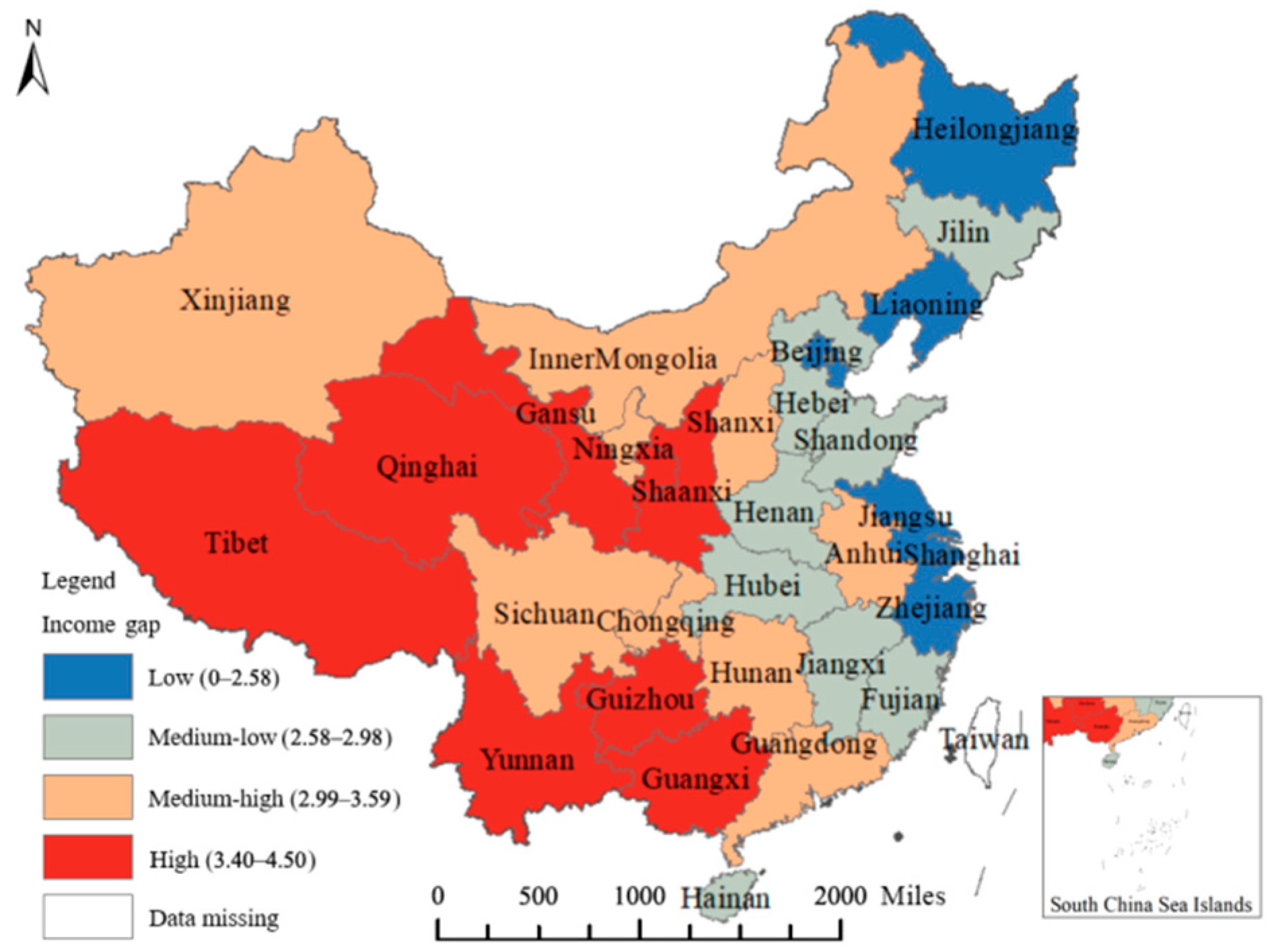
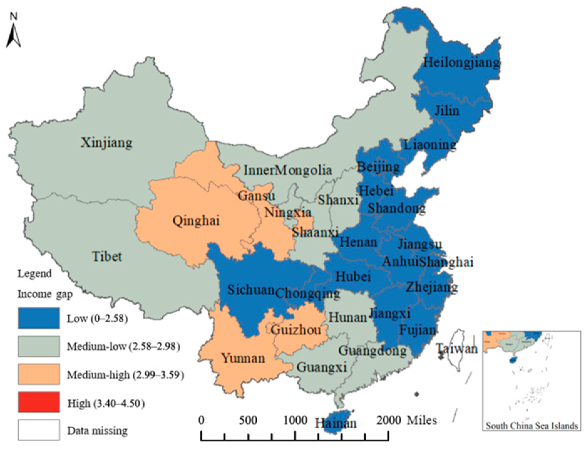
5.1. Global Spatial Correlation Test

The calculation results of $\mathrm{Moran}\prime \mathrm{s} \mathrm{I}$ by Formula (1) are displayed in

Table 3. Moran’s I of Provincial Urban–Rural Income Gap between 2007 and 2018.

Year	Moran’s I	Year	Moran’s I
2007	0.586 ***	2013	0.522 ***
2008	0.584 ***	2014	0.415 ***
2009	0.558 ***	2015	0.438 ***
2010	0.541 ***	2016	0.429 ***
2011	0.530 ***	2017	0.416 ***
2012	0.529 ***	2018	0.404 ***

*** indicate significance at the confidence levels of 1%.

, which indicates the urban–rural income gap in 31 provincial regions in China from 2007 to 2018. The value of $\mathrm{Moran}\prime \mathrm{s} \mathrm{I}$ is significantly positive at the 1% level, which indicates that the provincial-level urban–rural income gap has a positive spatial correlation. Geographically, provinces with large and low urban–rural income gaps have combined effects. At the same time, the $\mathrm{Moran}\prime \mathrm{s} \mathrm{I}$ of China’s urban–rural income gap typically displays a downward trend over the study period, indicating a weakening of the spatial positive correlation trend of China’s provincial-level urban–rural income gap.

Furthermore, ArcGIS 10.7 (ESRI, Redlands, CA, USA) was employed to depict the urban–rural income gap of 31 provincial regions in the Chinese mainland through images. In order to obtain more clustering information on the urban–rural income gap among provinces, this paper took 2007 as a reference and divided the urban–rural income gap into four levels: low (0–2.58), medium-low (2.59–2.98), medium-high (2.99–3.59), and high (3.40–4.5), according to the natural breaks (Jenks) classification method. At the same time, this paper provides a hierarchical graph of the provincial-level urban–rural income gap in 2018 to facilitate the comparative observation of the spatiotemporal variation characteristics of the provincial-level urban–rural income gap.

According to Figure 1 and Figure 2, China’s provincial urban–rural income gap generally presented a downward trend between 2007 and 2018. The original “high” level of urban–rural income gap disappeared, and the number of provinces with a “medium-high” level of urban–rural income gap reduced from nine in 2007 to four in 2018. Correspondingly, the number of provinces with “medium-low” or “low” levels increased. The urban–rural income gap levels of seven provinces remained unchanged from 2007 to 2018, and 24 provinces experienced different degrees of decline. Among them, the urban–rural income gap of Sichuan and Chongqing decreased by two levels from “medium-high” to “low”, that of Tibet, Shaanxi, and Guangxi decreased by two levels from “high” to “medium-low”, and those of the remaining 19 provinces only decreased by one level. In conclusion, China’s overall urban–rural income gap significantly narrowed over the study period.

As for spatial distribution, in 2007, provinces with a “high” urban–rural income gap were concentrated in the western region (except Sichuan, Chongqing, Xinjiang, and Inner Mongolia); provinces with a “low” income gap were mainly concentrated in a small part of eastern China, such as the Beijing–Tianjin–Liaoning region, the Yangtze River Delta, and Heilongjiang Province; provinces with a “medium-low” income gap were situated separately in parts of central and eastern China. In contrast, in 2018, about 84% of the provinces in the eastern and central regions presented a “low” urban–rural income gap, with an area significantly larger than that in 2007. Provinces in the western region cover three levels of the urban–rural income gap. Among them, provinces with a “medium-low” urban–rural income gap accounted for 50% of the whole. Additionally, the levels of urban–rural income gaps in Sichuan and Chongqing, which are “low”, and those of Yunnan, Guizhou, Qinghai, and Gansu on the north and south sides, which are “medium-high”, remain two levels apart, indicating that the imbalance in interprovincial urban–rural income gap in the western region is especially pronounced. In conclusion, the provincial urban–rural income gap in China is gradually widening from east to west, and there is a tendency of the radiating influence of the eastern region toward the central and western regions, driving the narrowing of the urban–rural income gap.

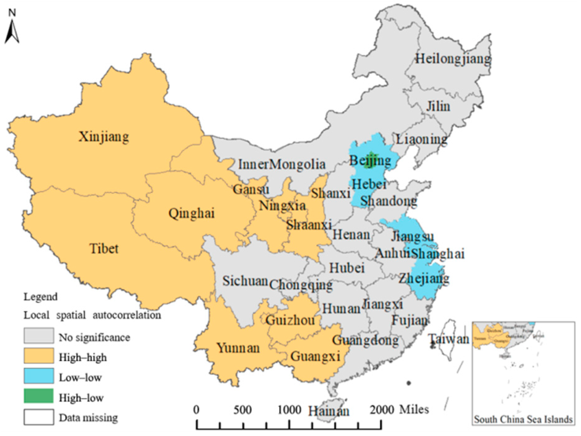
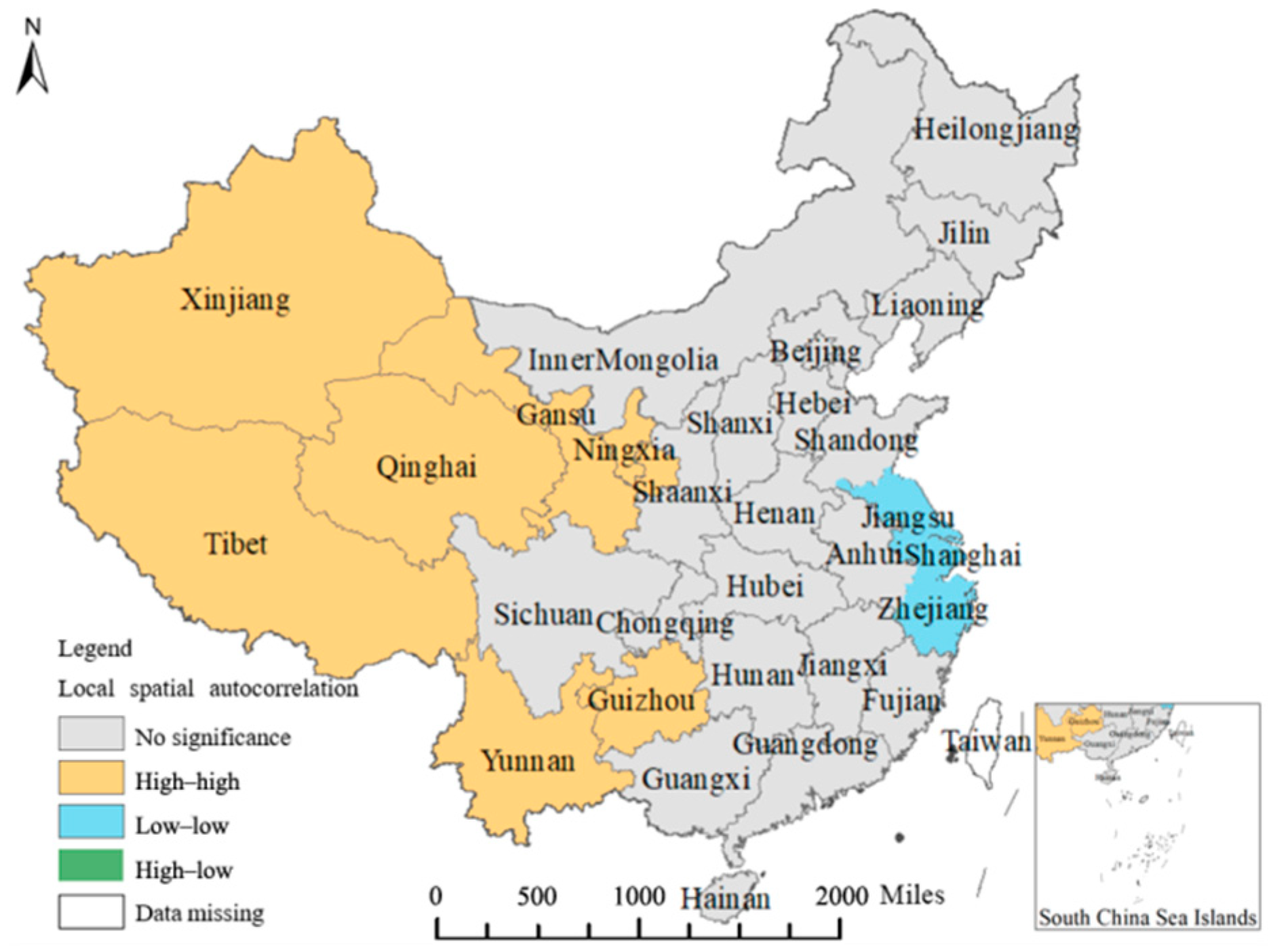
5.2. LISA Analysis of Spatial Correlation of Provincial Urban–Rural Income Gap

LISA image was utilized to analyze the spatial correlation of China’s provincial urban–rural income gap. According to Figure 3 and Figure 4, the urban–rural income gap in 13 (about 41.94%) and 10 (about 32.26%) provinces and cities passed the significance test of local spatial autocorrelation in 2007 and 2018, respectively, featuring two spatial correlations of “high–high” and “low–low”. “High–high” agglomeration means that the urban–rural income gap between these provinces and the surrounding provinces is on the high side, while “low–low” agglomeration means that the urban–rural income gap between these provinces and the surrounding provinces is on the low side, indicating that the provincial urban–rural income gap presents a geographically combined effect. In 2007, the numbers of provinces featuring “high–high” and “low–low” agglomeration were nine (about 53.85%) and five (about 38.46%), respectively. The provinces featuring “high–high” agglomeration were mainly located in western China, while the provinces featuring “low–low” agglomeration were mainly distributed in eastern China, such as Hebei, Tianjin, Jiangsu, Shanghai, and Zhejiang. Notably, Beijing (about 7.7%) exhibited “high–low” agglomeration in 2007, indicating a higher urban–rural income gap in Beijing than in surrounding provinces. In 2018, the numbers of provinces featuring “high–high” and “low–low” agglomeration wereseven (70%) and three (30%), respectively. The provinces featuring “high–high” agglomeration were mainly distributed in most provinces in west China, while the provinces featuring “low–low” agglomeration were mainly located in Jiangsu, Shanghai, and Zhejiang in the east. In general, “high–high” and “low–low” agglomeration areas were distributed in western and eastern provinces, respectively, from 2007 to 2018, which displayed a spatial trend of shrinking, reflecting that China’s provincial urban–rural income gap demonstrated an obvious trend of west–east differentiation.

5.3. Empirical Results and Analysis

The results of the aforementioned spatial autocorrelation test indicate a spatial correlation and heterogeneity in China’s urban–rural income gap. Therefore, incorporating spatial correlation into the regression model is crucial. By referring to the practice of existing literature, this paper carries out a likelihood ratio (LM) test, a Hausman test, and a Wald test in order to determine the specific estimation form of the spatial econometric model. Specifically, the results of the Wald test and the LR test suggest that the SDM model can neither be transformed into the SLM model nor the SEM model. Secondly, the Hausman test is employed to determine whether the SDM model should be estimated based on random effects or fixed effects. The statistics are significant at the 1% level, indicating that the original hypothesis is rejected and the model should be based on fixed effects. Finally, in order to choose one of the three effects for the SDM model, the time-fixed, entity-fixed, and time–entity-fixed effects are screened using the LR joint significance test. The test results in

Table 4. Results of Wald test, LR test, and Hausman test.

Test	Statistics	p Value
Wald test spatial lag	101.6996	0.0000
LR test for spatial lag	25.11	0.0007
Wald test spatial error	23.5889	0.0000
LR test for spatial error	41.16	0.0000
Hausman test	19.53	0.0015
Entity fixed effect testing	42.77	0.0000
Time fixed effect testing	700.67	0.0000

suggest that the original assumptions of entity fixed effects and time fixed effects are rejected, respectively, indicating that the time–entity-fixed effects should be adopted for the SDM model.

In order to verify the optimality of the alternative models with the estimation results, models (3)–(5) are used in this paper, and the Lee and Yu conversion estimation method is used for the spatial econometric model proposed in this paper, with the OLS estimation results added.

Table 5. Estimation Results of Panel Data Regression and Spatial Econometric Model.

Variables	OLS	SLM	SEM	SDM (1)	SDM (2)
C	5.0525 ***(3.99)
URB	−0.6318 *** (−15.62)	−0.4413 *** (−7.90)	−0.5847 *** (−10.75)	−0.3731 *** (−5.14)	−0.3048 *** (−4.04)
PHCG	−0.09270 *** (−2.97)	−0.0820 (0.016)	−0.1140 *** (−3.13)		−0.0536 (−1.38)
UNE	−0.00478 * (−1.86)	−0.0021 (−0.88)	−0.0056 * (−1.70)		−0.0097 ** (−2.48)
FCI	−0.1081 (−0.66)	−0.1189 *** (−0.77)	−0.2697 (−1.60)		−0.1145 (−0.69)
PEDU	−0.0065 (−0.99)	−0.0049 (−0.83)	−0.0036 (−0.61)		−0.0062 (−1.05)
ARG	−0.1865 (−1.15)	−0.3876 ** (−2.54)	−0.2977 * (−1.88)		−0.4887 *** (−3.12)
IU	0.0680 ** (2.38)	0.0539 * (1.97)	−0.0673 ** (2.44)		0.0276 (1.01)
W* URB				−0.2661 *** (−3.07)	−0.3507 *** (−3.31)
W* PHCG					−0.0551 (−0.93)
W*UNE					0.0094 ** (2.09)
W* FCI					0.6188 ** (2.30)
W* PEDU					0.0024 (0.23)
W* ARG					0.6404 ** (2.24)
W* IU					−0.0514 (−0.72)
Spatialrho		0.3289 *** (5.66)	0.2825 *** (3.65)	0.2542 *** (3.92)	0.2798 *** (4.20)
Variance sigma2_e		0.0020 *** (12.95)	0.0020 *** (12.92)	0.0021 *** (12.98)	0.0019 *** (12.96)
R2	0.7512	0.7637	0.7499	0.7583	0.7785
Log L	970.87	573.1603	565.1397	567.8444	585.7177

Note: *, **, and *** refer to significance at the confidence levels of 10%, 5%, and 1%, respectively.

displays the estimation results of panel regression and the spatial econometric model under the time–entity-fixed effects, where SDM (1) represents the SDM model without control variables and SDM (2) represents the SDM model with control variables. Table 5 demonstrates that the URB, the core explanatory variable of different models, is negative at the significance level of 1%, indicating that there is a significant negative relationship between the URB and the IG. Moreover, theR² (goodness of fit) values of the five models are all above 0.75. Among them, only theR² value of SDM (1) is as high as 0.7583, accounting for about 97.4% of the R²of SDM (2), which implies the significance of the core explanatory variable in all explanatory variables due to its high interpretability. Since the R²and Log L of SDM (2) are the highest, SDM (2) with time- and entity-fixed effects is selected as the interpretation model of this paper. The SDM (2) estimation results of time- and entity-fixed effects show that at the confidence level of 5%, the URB, UNE, and ARG are all significant. The improvement of these three variables is conducive to narrowing the urban–rural income gap in a province. The spatial lag coefficient of URB is negative at the significance level of 1%, which indicates that the improvement of URB in a province can also promote the narrowing of the urban–rural income gap in adjacent provinces. The spatial lag coefficients of UNE, FCI, and ARG are positive at the significance level of 5%, indicating that the improvement of these three variables has an expanding impact on the urban–rural income gap in adjacent provinces, of which the UNE has the smallest impact. The remaining variables are all non-significant.

In order to deeply analyze the spatial spillover effects of each variable, this paper decomposes the SDM (2) model to obtain the corresponding direct effect, indirect effect, and total effect (which is the sum of the direct effect and indirect effect), as shown in

Table 6. Effect Decomposition of Spatial Durbin Model.

Variables	Direct Effects	Indirect Effects	Total Effects
URB	−0.3328 *** (−4.50)	−0.5782 *** (−4.74)	−0.9110 *** (−8.11)
PHCG	−0.0595 (−1.61)	−0.0840 (−1.17)	−0.1434 * (−1.90)
UNE	−0.0088 ** (−2.47)	0.0087 * (1.75)	−0.0002 (−0.04)
FCI	−0.0783 (−0.50)	0.7595 ** (2.19)	0.6812 * (1.81)
PEDU	−0.0060 (−1.04)	0.0018 (0.12)	−0.0043 (−0.24)
ARG	−0.4491 *** (−2.93)	0.6512 * (1.76)	0.2020 (0.48)
IU	0.0250 (0.81)	−0.0544 (−0.54)	−0.0295 (−0.25)

Note: *, **, and *** refer to significance at the confidence levels of 10%, 5%, and 1%, respectively.

. It can be seen that the direct and indirect effects of URB are negative, but the absolute value of this indirect effect is larger, reflecting that the higher the urbanization level of a province, the smaller the urban–rural income gap in that province, and the greater the effect on narrowing the urban–rural income gap in adjacent provinces. The main reason is that the urbanization process of a province involves the transfer of more investment, industry, human capital, and other resources to rural areas and small towns, which is conducive to the rational layout of township industries and the increase in rural residents’ income. Additionally, the province’s increased URB will draw more capital, labor, and other resources from surrounding provinces, which would initially strain those provinces’ resources and reduce the urban–rural income gap caused by the lagging of the overall development; secondly, the interprovincial flow of resources helps to improve the return rate of capital and the income level of labor, thereby increasing the income and consumption level of adjacent provinces’ residents, especially interprovincial migrant workers; thirdly, the higher the province’s degree of urbanization in the later stage, the more likely it is to form a regional central city. The interprovincial layout of industries is improved through industrial transfer to the surrounding, less developed provinces. Industrial transfer to the surrounding less developed provinces helps to improve the industrial layout across provinces, and plays a radiation role by driving the overall urban–rural development in the adjacent provinces, thereby narrowing the urban–rural income gap.

For other control variables, the direct and indirect effects of UNE are positive and negative at the levels of 5% and 10%, respectively, indicating that the increased UNE can reduce the urban–rural income gap in a province while widening that in adjacent provinces. On the one hand, this is mainly because the employment environment in the province is poor, with few job positions, which indirectly reflects that the province is encountering a bottleneck in its economic development, and the urban–rural development gap is small. Therefore, the reduction in the urban–rural income gap in the province is based on the insufficient development of both urban and rural areas. On the other hand, the rise of UNE in the province will lead to the outflow of funds and labor to relatively developed cities in adjacent provinces, increase competition and efficiency, and thus improve the development rate and quality of adjacent provinces. This further results in a wider urban–rural development gap, which will inhibit the reduction in the urban–rural income gap in adjacent provinces. However, the spatial spillover effect of UNE is severely constrained due to the small absolute values of direct and indirect effect coefficients.

The indirect effect of FCI is positive at the level of 5%, suggesting that the increased FCI in a province will widen the urban–rural income gap in adjacent provinces. The reasonable explanation is that the increased FCI in a province boosts the development potential and investment attractiveness, and has a crowding-out effect on the human, technical, financial, and other resources of adjacent provinces. This further degrades the neighboring provinces’ development environments, particularly the soft and hard environments necessary for rural development, which widens the urban–rural income gap in adjacent provinces.

The direct effect of ARG is negative at the confidence level of 1%, and its indirect effect is positive at the confidence level of 10%, indicating that the improvement of ARG will help promote the development of this province’s primary industry, increase rural residents’ income, and reduce the urban–rural income gap. However, the development of farming, forestry, animal husbandry, and fishery in this province also has a crowding-out effect on that of adjacent provinces, resulting in lagging development and making it difficult to narrow the urban–rural income gap. The direct and indirect effects of other variables are all non-significant.

5.4. Robustness Test

To test the robustness of the above-mentioned empirical results, this paper estimates the SDM (2) model and decomposes the spatial effects by replacing the 0–1 adjacency matrix with the spatial weight matrices of economic distance and geographical distance.

Table 7. Effect Decomposition of SDM based on Spatial Weight Matrices of Economic and Geographic Distances.

Variables	Spatial Matrix of Economic Distance			Spatial Matrix of Geographic Distance
	Direct Effects	Indirect Effects	Total Effects	Direct Effects	Indirect Effects	Total Effects
URB	−0.3012 *** (−4.32)	−0.5414 *** (−3.89)	−0.8426 *** (−6.63)	−0.2575 *** (−3.32)	−0.6908 *** (−5.06)	−0.9483 *** (−8.65)
PHCG	−0.0265 (−0.70)	−0.0534 (−0.60)	−0.0799 (−0.93)	−0.0821 ** (−2.20)	0.0522 (0.65)	−0.0299 (−0.40)
UNE	−0.0091 *** (−2.47)	0.015 *** (3.11)	0.0059 (1.43)	−0.0110 *** (−3.12)	0.0148 *** (2.96)	0.0038 (1.00)
FCI	−0.0542 (−0.33)	0.2869 (0.74)	0.2327 (0.59)	0.0473 (0.30)	0.4199 (1.15)	0.4672 (1.25)
PEDU	0.0007 (0.12)	−0.020 (−0.84)	−0.0193 (−0.76)	−0.0065 (−1.15)	0.0150 (0.81)	0.0085 (0.44)
ARG	−0.4621 *** (−3.05)	0.4534 (1.01)	−0.0087 (−0.02)	−0.5037 *** (−3.32)	1.1174 *** (3.54)	0.6137 (1.71)
IU	0.0329 (1.10)	0.0549 (0.50)	0.0878 (0.71)	0.0264 (0.90)	0.0407 (0.45)	0.0671 (0.65)
R2	0.7838			0.7868
Log L	585.0470			587.7501

Note: **, and *** indicate significance at the confidence levels of 5%, and 1%, respectively.

displays the decomposition results (direct effects, indirect effects, and total effects). By comparing the effect decomposition results under the two spatial weight matrices in Table 7 and the 0–1 matrix in Table 6, it is clear that the significance values of the direct effect, indirect effect, and total effect of URB under the three spatial weights are consistent with the symbols of coefficients, and the coefficient values are relatively close. Among the control variables, the direct and indirect effects of UNE are both significant at the level of 10%, with consistent symbols and close values of the coefficients. The direct effect of ARG is significant at the level of 1%, but its indirect effect is significant only under the adjacency and distance matrices, indicating that the indirect effect of ARG is related to spatial distance and has a low correlation with the economy. In contrast, the indirect effect of FCI is significant under the 0–1 matrix, but non-significant under the other two spatial matrices, indicating that the spatial effects of FCI are affected by the neighborhood relations of provinces. In conclusion, the effect decomposition results of the three spatial weight matrices are similar, which confirms the robustness of the estimation and analysis results of the SDM (2) model.

6. Mechanism Test

6.1. Human Capital Cumulative Effect

Urbanization will result in more public education facilities being built, better school operating circumstances, and more opportunities for rural education [44]. Urbanization has also accelerated the construction of infrastructure. The platform effect of the internet and other facilities has raised the standard of education and teaching in rural areas, greatly increased the level of human capital and rural residents’ capacity to achieve high incomes, and consequently decreased the urban–rural income gap (Cao and Shen, 2014) [45]. According to Tian’s (2010) analysis of national urban data, urban and rural residents’ rates of return to education were closer following urbanization, at 6% and 5.6%, respectively [44].

Table 8. Mediating Effect of Human Capital.

	(1)	(2)
	Hcapital	IG
URB	0.004 *	−0.020 ***
	(0.002)	(0.005)
Hcapital		0.168 *
		(0.100)
Controls	Yes	Yes
WURB	−0.012 ***	−0.032 ***
	(0.004)	(0.010)
WHcapital		0.095
		(0.200)
WControls	Yes	Yes
ρ	−0.092	0.129 *
	(0.076)	(0.074)
Fixed Effects—Province	Yes	Yes
Fixed Effects—Time	Yes	Yes
R2	0.059	0.068
N	372	372

Note: ***, and * indicate significance at the confidence levels of 1%, and 10%; data in parentheses refers to the robust standard error; the control variable is consistent with the regression results of the benchmark model.

displays the test results for the mediating effect of the human capital level. After controlling for the spatial spillover effects of each variable, the impact of URB on $\mathrm{IG}$ is positive at the significance level of 10% (Column 1), indicating that urbanization can significantly improve $\mathrm{Hcapital}$. Additionally, the impact of $\mathrm{Hcapital}$ on $\mathrm{IG}$ is positive at the significance level of 10% (Column 2), and the impact of $\mathrm{URB}$ on $\mathrm{IG}$ is negative at the significance level of 1% (Column 2), indicating that there is a mediating effect of $\mathrm{Hcapital}$ in the relationship between URB and $\mathrm{IG}$.

Furthermore, the impact of $\mathrm{WURB}$ on $\mathrm{Hcapital}$ is negative at the significance level of 1% (column 1), and the impact of $\mathrm{WURB}$ on $\mathrm{IG}$ is negative at the significance level of 1% (Column 2), indicating that urbanization has significant negative spatial spillover effects on $\mathrm{Hcapital}$; that is, the provincial urbanization construction and development not only improves the local $\mathrm{Hcapital}$, but also inhibits the $\mathrm{Hcapital}$ in other regions. While urbanization has narrowed the local $\mathrm{IG}$, it has also had a significant negative impact on the $\mathrm{IG}$ in other regions, and the impact effect is stronger.

6.2. Industrial Structure Optimization Effect

Urbanization allows rural surplus labor to participate in the production of urban sectors, offers a vast pool of cheap labor for the growth of the tertiary industry, optimizes the industrial structure, and raises the income level of peasant migrants [46]. The increased supply of urban labor has increased competition in the urban labor market and lowered urban wage levels. Simultaneously, urbanization has eased the tense man–land relationship in rural areas, optimized the distribution of labor resources, improved labor productivity, and increased rural residents’ income. As a result, the urban–rural income gap has been narrowed [47].

According to the test results of the mediating effects of the industrial structure shown in

Table 9. Mediating Effect of Industrial Structure.

	(1)	(2)
	Indus	IG
URB	−0.011 **	−0.019 ***
	(0.005)	(0.005)
Indus		−0.102 *
		(0.055)
Controls	Yes	Yes
WURB	0.015	−0.031 ***
	(0.010)	(0.010)
Windus		−0.358 ***
		(0.118)
WControls	Yes	Yes
ρ	0.093	0.072
	(0.075)	(0.076)
Fixed Effects—Province	Yes	Yes
Fixed Effects—Time	Yes	Yes
R2	0.007	0.066
N	372	372

Note: ***, **, and * indicate significance at the confidence levels of 1%, 5%, and 10%; data in parentheses refer to the robust standard error; the control variable is consistent with the regression results of the benchmark model.

, when the spatial spillover effect of each variable is controlled, $\mathrm{URB}$ has a negative impact on $\mathrm{indus}$ at the level of 5% (Column 1), indicating that the urbanization of provincial cities can optimize the industrial structure of the region. Moreover, the impact of $\mathrm{urbanrate}$ on $\mathrm{IG}$ is negative at the significance level of 1% (Column 2), and the impact of $\mathrm{indus}$ on $\mathrm{IG}$ is negative at the level of 10% (Column 2), confirming that there is a mediating effect of $\mathrm{indus}$ in the relationship between $\mathrm{URB}$ and $\mathrm{IG}$.

Additionally, the negative impact of $\mathrm{WURB}$ on $\mathrm{IG}$ is significant at the level of 1% (Column 2), and $\mathrm{Windus}$ has a negative impact on $\mathrm{IG}$ at the level of 1% (Column 2). The results demonstrate that, with a greater impact, the urbanization of provincial cities can optimize the local industrial structure, promote the adjustment of the industrial structure, and thus narrow the urban–rural income gap in the adjacent areas.

6.3. Effect of Technological Development

The improvement of urbanization level leads to the overflow of rural population to cities, increasing the number of resources that can be distributed per unit of rural residents under the condition that land and other factors remain unchanged. Farmers anticipate that technological progress will enable them to enhance their current farming practices in order to maximize revenues and make the most use of scarce resources, such as land. A certain degree of regional barriers between urban and rural areas can already be broken by increasing urbanization levels, which will also accelerate the flow of technology and wealth from urban to rural areas [12]. By introducing a large number of external technologies, farmers have realized mechanization and scale production, which has improved production efficiency, increased their income, and alleviated the urban–rural income gap [41].

According to the test results of the mediating effect of technological development (

Table 10. Mediating Effect of Technical Level.

	(1)	(2)
	Ininapply	IG
URB	0.065 ***	−0.017 ***
	(0.010)	(0.006)
lninapply		−0.054 **
		(0.025)
Controls	Yes	Yes
WURB	0.068 ***	−0.038 ***
	(0.020)	(0.012)
Wlninapply		0.061
		(0.062)
WControls	Yes	Yes
ρ	−0.079	0.150 **
	(0.082)	(0.074)
Fixed Effects—Province	Yes	Yes
Fixed Effects—Time	Yes	Yes
R2	0.436	0.118
N	372	372

Note: ***, **, indicate significanceat the confidence levels of 1%, 5%; data in parentheses refer to the robust standard error; the control variable is consistent with the regression results of the benchmark model.

), $\mathrm{URB}$ has a positive impact on $\mathrm{lninapply}$ at the level of 1% (Column 1), which indicates that the urbanization of provincial cities can promote their technological development. Moreover, the negative impact of $\mathrm{URB}$ on $\mathrm{IG}$ is significant at the level of 1% (Column 2), and the impact of $\mathrm{lninapply}$ is negative at the significance level of 5% (Column 2), which proves that there is a technical mediating effects on the relationship between $\mathrm{URB}$ and $\mathrm{IG}$.

Additionally, the positive impact of $\mathrm{WURB}$ on $\mathrm{lninapply}$ is significant at the level of 1% (Column 1), and $\mathrm{WURB}$ has a negative impact on $\mathrm{IG}$ at the significance level of 1% (Column 2), indicating that the urbanization of provincial cities can boost the degree of technical innovation in neighboring cities and encourage a reduction in the urban–rural gap in the region. The urbanization of the region has a much greater effect on the reduction in the urban–rural gap in other regions.

7. Discussion

Through the benchmark regression and robustness test, we found that the improvement of urbanization level can significantly reduce the urban–rural income gap. The reasons for this may be related to a provincial urbanization process involved in investment, with the transfer of industrial and human capital, and other resources, to the countryside and small towns. The reasonable layout is conducive to the villages’ and towns’ industry, and rural populations increase, which leads to the reduction in the urban–rural income gap. At the same time, the improvement of the provincial urbanization level has a significant effect on the reduction in the urban–rural income gap in neighboring provinces. This may be because the increase in the urbanization rate of this province will attract more capital, labor and other resources from neighboring provinces. In the early stage of urbanization, the rapid development of a local province may crowd out the resources of neighboring provinces, resulting in the narrowing of the urban–rural income gap caused by the overall backward development of neighboring provinces.

However, with the continuous improvement of urbanization, the inter-provincial flow of resources becomes more and more frequent, which helps to improve the rate of return of capital and the income level of labor in neighboring provinces, thus increasing the income and consumption level of urban and rural residents in neighboring provinces, especially inter-provincial migrant workers. Crucially, if the province’s urbanization degree is higher, the more conducive it will be to forming regional central cities. The central cities can improve the inter-provincial industrial layout by transferring industries to the neighboring, less developed provinces, which further has a radiating effect on the development of the neighboring provinces, driving the development of the surrounding overall urban and rural areas and narrowing the gap between the urban and rural income levels of the neighboring provinces.

The results of the mechanism test show that the improvement in urbanization rate can effectively reduce the urban–rural income gap through the accumulation effect of human capital, the optimization effect of industrial structure and the improvement effect of technological level. First of all, as far as the accumulation effect of human capital is concerned, the development of urbanization will expand the construction of various public education facilities, improve the school conditions of rural education, and increase the possibility of rural education [44]. At the same time, urbanization has led to the rapid development of infrastructure. The platform effect of the internet and other facilities has improved the quality of education and teaching in rural areas, significantly improved the level of human capital, enhanced the ability of rural residents to obtain high income levels, and thus narrowed the urban–rural income gap [45].

Second, we consider the industrial structure optimization effect. Urbanization gives the surplus rural labor force the opportunity to participate in urban sector production, which provides a large amount of cheap labor resources for the development of tertiary industry. According to the Lewis Model, urban industrial sectors with high marginal productivity and agricultural sectors with low marginal productivity are common in developing countries, and the labor force will gradually transfer from the agricultural sector with low marginal productivity to the urban industrial sector with high marginal productivity until the surplus rural labor is completely absorbed. Urbanization leads to the rapid development of the urban industrial sector, which increases the demand for labor and accelerates the above process. Urbanization gives the surplus rural labor force the opportunity to participate in urban sector production, which provides a large amount of cheap labor resources for the development of tertiary industry, optimizes the industrial structure, and helps to improve the income level of farmers in the city [46]. At this time, the increase in urban labor supply intensifies the degree of competition in the urban labor market and reduces the urban wage level, while urbanization can ease the current situation of human and land constraints in rural areas, optimize the allocation of labor resources, improve labor productivity, and increase the rural income level, which further reduces the urban–rural income gap [47].

Finally, from the perspective of the effect of technology improvement, it may be that the improvement of urbanization level leads to the overflow of rural population to cities, and the allocable resource endowments per unit of rural population increases when land and other factors remain unchanged. In order to make full use of land and other limited resources, and maximize profits, farmers can improve traditional farming methods through technological innovation. At this time, the improvement of the urbanization level can break the regional barriers between urban and rural areas, increase the flow of technology and other factors, and to some extent promote the flow of capital and technology from cities to rural areas [12]. Farmers can achieve mechanization and scale through the introduction of a large number of external technologies, which improves production efficiency, further increases rural income, and eases the urban–rural income gap [41].

8. Conclusions and Recommendations

The existing literature fails to account for spatial correlation when examining how urbanization affects the urban–rural income gap (IG), resulting in a bias in the estimation results and a lack of reliability in the research conclusions. Therefore, this paper has established a spatial econometric model using panel data from 31 provinces and cities in China from 2007 to 2018 to test the spatial spillover effect of urbanization and IG. The main conclusions of this paper are as follows: Firstly, the change graphs of IG show that, with the exception of 7provinces, the levels of IG have remained unchanged, while the remaining 24 provinces and cities have experienced varying degrees of decline, indicating that China’s IG is shrinking at the provincial level. However, it is noteworthy that the provincial-level IG in China is almost twice as large as that in industrialized nations at the same stage, indicating that China’s IG is still substantial, and the problem of the dualistic structure system of urban and rural areas remains to be solved.

Secondly, according to the test results of global spatial autocorrelation indicators, the spatial correlation between the provincial IG in China is positive. Provinces with a large IG, featuring “high–high” agglomeration, are mostly concentrated in western regions, while provinces featuring “low–low” agglomeration are located primarily in the Yangtze River Delta region. As the positive spatial correlation weakens, provinces exhibit a distinct trend of east–west differentiation.

Thirdly, according to the test results of the spatial econometric model, IG can be reduced in a province by increasing its urbanization level. This is in line with the findings of Ahmed et al. (2020) [26] and Guo et al. (2022) [11], and this improvement has a stronger impact on the reduction in IG in adjacent provinces. Additionally, the rise in the urban unemployment rate (UNE) has narrowed IG in this province and expanded IG in adjacent provinces. The improvement of the gross output value of farming, forestry, animal husbandry, and fishery (ARG)has a promoting effect on narrowing the IG in this province, but it will have a greater inhibitory effect on the narrowing of the IG in adjacent provinces. The aforementioned conclusions are made robust after replacing the 0–1 adjacency matrix with the spatial weight matrices of economic distance and geographical distance, respectively.

Finally, the results of the mediating effect tests demonstrate that urbanization can narrow the urban–rural income gap by improving the region’s human capital, optimizing the region’s industrial structure, and promoting urban technological development. This is in line with the findings of Ahmed et al. (2020) [26] and Bosker and Buringh (2017) [27]. While the development of provincial cities reduces the urban–rural income gap, the urbanization level in the region has a stronger narrowing effect on the urban–rural income gap in surrounding cities. At the same time, as this paper uses provincial-level data, it is not possible to study in-depth the impact of urbanization on the urban–rural income gap in different contexts. Therefore, we will collect data at the village and county levels as possible ways to explore the different heterogeneous impacts in the future.

According to the empirical analysis in this paper, there is an objective spatial spillover effect of the UNE and IG in China, with regional differences. Therefore, we give the following recommendations in this paper: given the effect of improving the urbanization rate in reducing the urban–rural income gap in a province and its surrounding provinces, accelerating new urbanization, and promoting the equalization of urban and rural public services on the basis of sufficient ecological environment and resource carrying capacity, can increase the positive externalities released by urbanization, which thus radiate into and lead the coordinated development of township areas, and realizes the sharing of development achievements between urban and rural residents. Provinces can increase employment through measures such as industrial optimization and infrastructure construction, which can not only improve the employment rate of urban and rural residents in the province, but also accelerate the interprovincial flow of rural surplus labor, allowing for better labor resource allocation and increased competition and efficiency. Additionally, against the background of the rural revitalization strategy, it is recommended to optimize the layout and development environment of the primary industry so as to promote its coordinated development with the secondary and tertiary industries. We should also promote modern agricultural technology and management systems that are appropriate for local conditions, and improve the scope and caliber of farming, forestry, animal husbandry, and fisheries by adopting cutting-edge machinery and equipment, which will raise residents’ income and narrow the income gap between industries, as well as between urban and rural areas.

References

1. Derudder, B.; Cao, Z.; Liu, X.; Shen, W.; Dai, L.; Zhang, W.; Caset, F.; Witlox, F.; Taylor, P.J. Changing connectivities of Chinese cities in the world city network, 2010–2016. Chin. Geogr. Sci. 2018, 28, 183–201. [Google Scholar] [CrossRef] [Green Version]
2. Raźniak, P.; Csomós, G.; Dorocki, S.; Winiarczyk-Raźniak, A. Exploring the shifting geographical pattern of the global command-and-control function of cities. Sustainability 2021, 13, 12798. [Google Scholar] [CrossRef]
3. Csomós, G. Cities as command and control centres of the world economy: An empirical analysis, 2006-2015. Bull. Geogr. Soc.-Econ. Ser. 2017, 38, 7–26. [Google Scholar] [CrossRef] [Green Version]
4. Luo, Z.; Wan, G.; Zhang, X.; Li, J. Urbanization with Efficiency and Equity: A Theoretical Model and Chinese Empirical Studies. Econ. Res. 2018, 7, 89–105. [Google Scholar]
5. Yuan, Y.; Wang, M.; Zhu, Y.; Huang, X.; Xiong, X. Urbanization’s effects on the urban-rural income gap in China: A meta-regression analysis. Land Use Policy 2020, 99, 104995. [Google Scholar] [CrossRef]
6. Chen, Z.; Meng, Q.; Xu, R.; Guo, X.; Cai, C. How rural financial credit affects family farm operating performance: An empirical investigation from rural China. J. Rural. Stud. 2022, 91, 86–97. [Google Scholar] [CrossRef]
7. Zhou, Q.; Shi, W. How does town planning affect urban-rural income inequality: Evidence from China with simultaneous equation analysis. Landsc. Urban Plan. 2022, 221, 104380. [Google Scholar] [CrossRef]
8. Cheng, M.; Zhang, J. Internet Popularization and Urban-Rural Income Gap: Theory and Empirical Studies. China Rural. Econ. 2019, 2, 19–41. [Google Scholar]
9. Ding, N.; Wang, Y. Household income mobility in China and its decomposition. China Econ. Rev. 2008, 19, 373–380. [Google Scholar] [CrossRef]
10. Luo, C.; Li, S.; Yue, X. Analysis of changes in the income gap of Chinese residents (2013–2018). Chin. Soc. Sci. 2021, 1, 33–54. [Google Scholar]
11. Guo, D.; Jiang, K.; Xu, C.; Yang, X. Industrial clustering, income and inequality in rural China. World Dev. 2022, 154, 105878. [Google Scholar] [CrossRef]
12. Zhong, S.; Wang, M.; Zhu, Y.; Chen, Z.; Huang, X. Urban expansion and the urban–rural income gap: Empirical evidence from China. Cities 2022, 129, 103831. [Google Scholar] [CrossRef]
13. Hong, T.; Yu, N.; Mao, Z.; Zhang, S. Government-driven urbanisation and its impact on regional economic growth in China. Cities 2021, 117, 103299. [Google Scholar] [CrossRef]
14. Zhou, Y.; Guo, L.; Liu, Y. Land consolidation boosting poverty alleviation in China: Theory and practice. Land Use Policy 2019, 82, 339–348. [Google Scholar] [CrossRef]
15. He, Y. Agricultural population urbanization, long-run economic growth, and metropolitan electricity consumption: An empirical dynamic general equilibrium model. Energy Strategy Rev. 2020, 30, 100498. [Google Scholar] [CrossRef]
16. Cao, Y.; Kong, L.; Zhang, L.; Ouyang, Z. The balance between economic development and ecosystem service value in the process of land urbanization: A case study of China’s land urbanization from 2000 to 2015. Land Use Policy 2021, 108, 105536. [Google Scholar] [CrossRef]
17. Pradhan, R.P.; Arvin, M.B.; Nair, M. Urbanization, transportation infrastructure, ICT, and economic growth: A temporal causal analysis. Cities 2021, 115, 103213. [Google Scholar] [CrossRef]
18. Jiang, Y.; Long, H.; Ives, C.D.; Deng, W.; Chen, K.; Zhang, Y. Modes and practices of rural vitalisation promoted by land consolidation in a rapidly urbanising China: A perspective of multifunctionality. Habitat Int. 2022, 121, 102514. [Google Scholar] [CrossRef]
19. Liu, Z. Human capital externalities in cities: Evidence from Chinese manufacturing firms. J. Econ. Geogr. 2014, 14, 621–649. [Google Scholar] [CrossRef]
20. Glaeser, E.L.; Lu, M. Human-capital externalities in China. Natl. Bur. Econ. Res. 2018, 11, 122–139. [Google Scholar]
21. Kanbur, R.; Zhang, X. Fifty years of regional inequality in China: A journey through central planning, reform, and openness. Rev. Dev. Econ. 2005, 9, 87–106. [Google Scholar] [CrossRef] [Green Version]
22. Zeng, C.; Song, Y.; He, Q.; Liu, Y. Urban–rural income change: Influences of landscape pattern and administrative spatial spillover effect. Appl. Geogr. 2018, 97, 248–262. [Google Scholar] [CrossRef]
23. Cai, Z.; Liu, Z.; Zuo, S.; Cao, S. Finding a Peaceful Road to Urbanization in China. Land Use Policy 2019, 83, 560–563. [Google Scholar] [CrossRef]
24. Singhal, K.; Singhal, J. Technology and Manufacturing in China before the Industrial Revolution and Glimpses of the Future. Prod. Oper. Manag. 2019, 28, 505–515. [Google Scholar] [CrossRef]
25. Hsu, W.-T.; Ma, L. Urbanization policy and economic development: A quantitative analysis of China’s differential hukou reforms. Reg. Sci. Urban Econ. 2021, 91, 103639. [Google Scholar] [CrossRef]
26. Ahmed, Z.; Zafar, M.W.; Ali, S. Linking urbanization, human capital, and the ecological footprint in G7 countries: An empirical analysis. Sustain. Cities Soc. 2020, 55, 102064. [Google Scholar] [CrossRef]
27. Bosker, M.; Buringh, E. City seeds: Geography and the origins of the European city system. J. Urban Econ. 2017, 98, 139–157. [Google Scholar] [CrossRef] [Green Version]
28. Gao, Y.; Zang, L.; Sun, J. Does computer penetration increase farmers’ income? an empirical study from china. Telecommun. Policy 2018, 42, 345–360. [Google Scholar] [CrossRef]
29. Sheng, Y.; Zhao, Y.; Zhang, Q.; Dong, W.; Huang, J. Boosting rural labor off-farm employment through urban expansion in China. World Dev. 2022, 151, 105727. [Google Scholar] [CrossRef]
30. Gao, W.; Smyth, R. Education expansion and returns to schooling in urban China, 2001–2010: Evidence from three waves of the China Urban Labor Survey. J. Asia Pac. Econ. 2014, 20, 178–201. [Google Scholar] [CrossRef]
31. Liao, Y.; Zhang, J. Hukou status, housing tenure choice and wealth accumulation in urban China. China Econ. Rev. 2021, 68, 101638. [Google Scholar] [CrossRef]
32. Glauben, T.; Herzfeld, T.; Rozelle, S.; Wang, X. Persistent Poverty in Rural China: Where, Why, and How to Escape? World Dev. 2012, 40, 784–795. [Google Scholar] [CrossRef] [Green Version]
33. Chen, B.; Lin, Y. Development strategy, urbanization and income gap between urban and rural areas in China. Chin. Soc. Sci. 2013, 4, 81–102. [Google Scholar]
34. Su, C.W.; Liu, T.Y.; Chang, H.L.; Jiang, X.Z. Is urbanization narrowing the urban-rural income gap? A cross-regional study of China. Habitat Int. 2015, 48, 79–86. [Google Scholar] [CrossRef]
35. Li, S.; Lin, S. Population aging and China’s social security reforms. J. Policy Model. 2016, 38, 65–95. [Google Scholar] [CrossRef]
36. Zhang, N. Urbanization, industrialization and urban-rural income gap: Inspection by panel var based on the provincial panel data. Stud. Sociol. Sci. 2016, 7, 210–237. [Google Scholar]
37. Luo, C. Economic Growth, Income Gap and Rural Poverty. Econ. Res. 2012, 2, 15–27. [Google Scholar]
38. Diamond, R. The determinants and welfare implications of US workers’ diverging location choices by skill: 1980-2000. Am. Econ. Rev. 2016, 106, 479–524. [Google Scholar] [CrossRef] [Green Version]
39. Wu, X.; Zheng, B. Household registration, urban status attainment, and social stratification in China. Res. Soc. Stratif. Mobil. 2018, 53, 40–49. [Google Scholar] [CrossRef]
40. Yang, G.; Bansak, C. Does wealth matter? An assessment of China’s rural-urban migration on the education of left-behind children. China Econ. Rev. 2020, 59, 101365. [Google Scholar] [CrossRef]
41. Han, F.; Li, Y. Industrial Agglomeration, Public Service Supply and Urban Scale Expansion. Econ. Stud. 2019, 11, 149–164. [Google Scholar]
42. Cheng, Z.; Guo, F.; Hugo, G.; Yuan, X. Employment and wage discrimination in the Chinese cities: A comparative study of migrants and locals. Habitat Int. 2013, 39, 246–255. [Google Scholar] [CrossRef]
43. Fraumeni, B.M.; He, J.; Li, H.; Liu, Q. Regional distribution and dynamics of human capital in China 1985–2014. J. Comp. Econ. 2019, 47, 853–866. [Google Scholar] [CrossRef]
44. Tian, F. A study on the income gap between urban workers and migrant workers. Sociol. Res. 2010, 2, 87–105. [Google Scholar] [CrossRef]
45. Cao, X.; Shen, K. Urban-rural income gap, labor quality and economic growth in China. Econ. Stud. 2014, 6, 30–43. [Google Scholar]
46. Mu, H.; Wu, P. Urbanization, industrial structure optimization and the urban-rural income gap. Economy 2016, 5, 37–44. [Google Scholar] [CrossRef]
47. Zhou, S.; Qi, S.; Lu, Z. Regional differences, urbanization and urban-rural income disparity. China Popul.—Resour. Environ. 2010, 8, 115–120. [Google Scholar]
Figure 1. Hierarchical graph of provincial urban–rural income gap in 2007. Data from China Statistical Yearbooks Database (CSYD).
Sustainability 14 13795 g001
Figure 2. Hierarchical graph of provincial urban–rural income gap in 2018.Data from China Statistical Yearbooks Database (CSYD).
Sustainability 14 13795 g002
Figure 3. LISA image of provincial-level urban–rural income gap in 2007.Data from China Statistical Yearbooks Database (CSYD).
Sustainability 14 13795 g003
Figure 4. LISA image of provincial-level urban–rural income gap in 2018.Data from China Statistical Yearbooks Database (CSYD).
Sustainability 14 13795 g004