Article

Ecological Security Pattern Construction in Beijing-Tianjin-Hebei Region Based on Hotspots of Multiple Ecosystem Services

1
School of Geograghical Science, Shanxi Normal University, Taiyuan 030000, China
2
Hebei Engineering Research Center for Geographic Information Application, Institute of Geographical Sciences, Hebei Academy of Sciences, Shijiazhuang 050011, China
*
Author to whom correspondence should be addressed.
Sustainability 2022, 14(2), 699; https://doi.org/10.3390/su14020699
Submission received: 9 November 2021 / Revised: 31 December 2021 / Accepted: 4 January 2022 / Published: 9 January 2022

Abstract

:
The contradiction between urban expansion and ecological protection in the Beijing-Tianjin-Hebei region (BTH) is increasingly acute, which has become one of the main problems restricting regional development, and sustainable development of ecosystem services is the key to increasing human well-being. Based on GIS platform and multiple models, this paper analyzes the temporal and spatial variation characteristics of four key ecosystem services (water conservation, soil conservation, habitat quality, and plant net primary productivity) in different ecological regions of BTH in recent 20 years, quantifies the impact of different climate factors and land use change on ecosystem services (ESs), and discusses the primary ecosystem hotspots and ecological security pattern. The results showed that the interannual variation of water conservation (WC) and plant net primary productivity (NPP) increased from 2000 to 2020, while the change of soil conservation (SC) was not obvious, which was mainly controlled by climate factors, WC and SC were more affected by precipitation, and temperature was the key factor affecting NPP. Habitat quality (HQ) presented a significant downward trend; it was mainly attributed to the deterioration of ecological environment caused by accelerated urbanization expansion. According to hotspot analysis, it could be found that WC was the fastest-growing ecosystem service function in BTH, and NPP would become the factor with the greatest contribution to ecological importance in the future. The important protected areas and main ecological sources of ecological security pattern were mainly distributed in Yanshan-Taihang mountain area, which was consistent with the key areas of ecosystem services. In this study, the temporal and spatial differences of ecosystem service in BTH were demonstrated in a more intuitive way and provided scientific guidance for decision makers to formulate effective ecological protection policies in different regions.

1. Introduction

Ecosystem Services (ES) can be defined as the result of positive interactions between humans and the ecosystem environment [1]. Ecosystem services, which can be divided into regulation services, supply services, support services, and cultural and entertainment services, play a fundamental role in helping human getting various benefits with a direct or indirect process [1,2,3]. However, the sustainable supply of ESs has been broken because as people gain the goods and benefits from ecosystem without restraint, ESs face more and more pressures due to the multiple changes of climate and land use, which are exacerbated by socio-economic developments and cause the destruction of ecosystem services such as soil and water loss, habitat conversion, degradation, and fragmentation [4,5,6]. In recent decades, about 60% of ecosystem services around the world have been degraded or unsustainable [2] and global ecosystems are showing declining trends at an unprecedented speed [7]. Scholars have started paying attention to the negative change of ESs worldwide [8,9,10], and the policy makers prefer to get more straightforward data to deepen the understanding of the relationship among different ecosystem services, which could help them ensure the sustainable development of desired ecosystem services [11,12,13].
Land use and climate change have been regarded as important driving factors of ESs provision and the relationship among different ESs [14,15]. Land use change is the main way that human activities affect ecosystem services; besides, the change of that affects ESs, such as regional water cycle, soil conservation, carbon storage, and so on through carbon balance and nutrient flow, e.g., Kusi et al. found that carbon storage might be promoted with the increase of urban areas, agriculture, sparse vegetation, and forests and the decrease of grassland and unused land, but water yield, sediment export, and nitrogen and phosphorus exports would suffer from a greater loss [16]. Further, land use change will also lead to landscape fragmentation and reduce the quality of habitat, in Pan-Yangtze River Delta region, the habitat quality decreased consistently and was fragmented in nearly 40 years due to land use change [17]. On the other hand, the global mean temperature is expected to increase in the future as the climate system responds with some delay to changes in atmospheric greenhouse gas [18,19]. The impact of climate change on ESs is directly through temperature, precipitation, solar radiation, and other factors on soil and water conservation and carbon dioxide concentration. In the Loess Plateau, there is a significant positive correlation between NPP and precipitation but a negative correlation with temperature factors, and the dominant climatic factor for ESs is annual precipitation [20]. Climate change and high-intensity land use development directly affect the regional landscape spatial pattern and ecological process and cause the originally fragile natural ecological environment to deteriorate [21].
A reasonable and orderly spatial pattern of ecological security plays an important role in maintaining ecosystem integrity, strengthening ecosystem spatial distribution pattern, and realizing ecological harmonious development [22]. The concept of ecological security based on maintaining the sustainable development of ecological process has gradually attracted extensive attention from the government and academia [23]. Multiple models have emerged to evaluate the ecological security pattern, such as circuit theory, overed weighted averaging (OWA), minimum cumulative resistance model (MCR), and so on [24,25,26]. At present, the method of using the minimum resistance model to determine the ecological source, establish the resistance surface, and then judge the security pattern proposed by Yu has become the main model for ecological security pattern construction and has been successfully applied to many regions, e.g., in northeast China and Guizhou Province [24,27,28]. In addition, ecosystem services are also added to the index system to build the ecological security pattern, Wang et al. used the priority and spatial richness indexes of ecosystem services to reconstruct the ecosystem services in Ganzhou and constructed ecological security patterns of different levels based on the reconstructed ecosystem services [29].
In summary, although people are increasingly concerned about the relationship between ecosystem services and their driving forces and realize the importance of ecological security pattern, there is no comprehensive framework that not only explains how climate and land use change affect ecosystem service function but also reveals the impact of ecological services on ecological security pattern. At present, the research methods of land use change on ecosystem service function are gradually mature, and model prediction has become the main direction of driving force analysis, such as CA_Markov model and CLUE_S model [30,31,32]. However, for the impact of climate change on ecosystem service, the research method is relatively single. Most studies focus on one or several ecosystem services and driving factors; the relationship between ecosystem service and a certain climate factor is mainly explained by correlation analysis or regression analysis [33,34]. These methods can only explain the relationship between climate and ecosystem services but cannot predict the impact of the change trend of a certain climate factor on ecological services in the future. Therefore, how to design scenarios to simulate the future changes of climate factors and effectively quantify the impact of different climate change scenarios on ecological services is the development trend of current research. Besides, although the MCR model has become the mainstream model to build the ecological security pattern, there is no standardized mode to choose ecological source and to build an ecological security pattern related to the protection of human well-being by combining ecological services [35].
Beijing-Tianjin-Hebei region (BTH) is not only the political, economic, and cultural center in China but also a particularly important ecological area. In the past 50 years, temperature in BTH has increased significantly, while precipitation and potential evapotranspiration have decreased in most sub-regions [36]. Simultaneously, the expansion speed of construction land is accelerated from 6.75% in 1975 to 12.9% in 2020 due to rapid urbanization. In order to alleviate the degradation of ESs due to urbanization, the ecological projects such as Grain to Green Project, Natural Forest Conservation Program, and Beijing-Tianjin Sand Source Control Program have been launched successively. Therefore, reasonable analysis of the impact of climate and land use change on ecosystem services, ecological security pattern construction in BTH, and scientific guidance for decision makers are of great significance to regional development.
The object of this study is to build a comprehensive evaluation to analyze the ecosystem service function of BTH from two aspects: driving force analysis and ecological security pattern construction. The process of model simulation is shown in Section 2. Section 3 mainly analyzes the temporal variation and spatial distribution of four kinds of ecosystem services (WC, SC, HQ, NPP); by different scenarios, the influence degree of driving factors was analyzed, and the ecological security pattern was constructed based on hotspot analysis. Section 4 mainly discusses the improvement of research method compared with the previous research methods, puts forward reference suggestions for the ecological civilization construction, and illustrates future research prospect. The Supplementary Information includes the following contents: (Supplementary Materials_A), calculation formula of ecosystem service model; (Supplementary Materials_B), proportion of hotspot area in different regions.

2. Materials and Methods
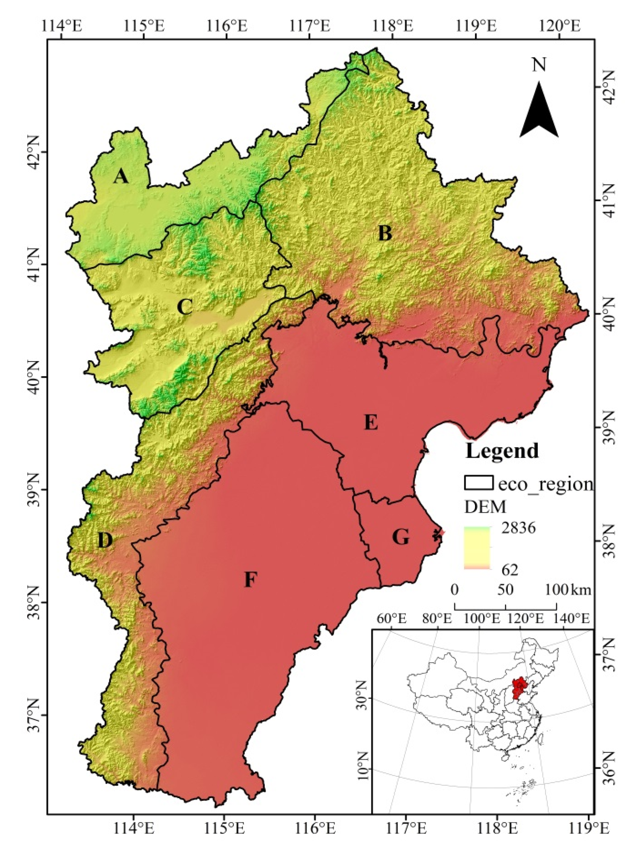
2.1. Study Area

The BTH is located in North China between 36.07 °N–42.65 °N and 113.46 °E–119.79 °E, and the elevation is from 52 m to 2836 m (Figure 1). The elevation is descending from north to south, which is characterized by the transition from mountain and hill to platform and plain. The climate type is humid and semi-arid continental monsoon climate with four distinct seasons [37]. Affected by elevation and climate factors, vegetation types are diverse, which can be divided into four vegetation zones: Bashang grassland, mountain and hilly deciduous broad-leaved forest, plain deciduous broad-leaved forest, and coastal plain halophyte [38]. With the continuous improvement of urbanization level, the proportion of construction land has risen from 8.17% in 2000 to 12.99% in 2020. About 10.2% of ecological land is converted to construction land, and the occupation of ecological land by urban expansion has become an important issue affecting the construction of ecological civilization.
According to the ecological regionalization by the Research Center for Eco-Environmental Sciences, Chinese Academy of Sciences (http://www.ecosystem.csdb.cn accessed on 20 December 2020), combined with topography, hydrothermal condition, vegetation characteristics, and ecosystem structure of BTH, the study area is divided into seven ecological regions (Figure 1).

2.2. Data Sources

The data required in this study mainly include meteorological, vegetation, land use, soil, DEM, and socio-economic data. The meteorological data was downloaded from China Meteorological Data Service Centre, including daily temperature, precipitation, and potential evapotranspiration data of 123 meteorological stations in BTH and its surrounding areas, and the data was rasterized by Kriging. The remote sensing data of NDVI, Land use, and DEM are raster data, soil and road data are vector data, and Water Resources is textual data from statistical yearbook. All data were consolidated into WGS84 coordinate system and Albert projection. The details are shown in Table 1.

2.3. Methods

2.3.1. Ecosystem Services Indicators

As an integral part of nature, ecosystem services can be used as an intermediate factor to connect ecosystem with human welfare, which has direct value to human and society, so as to bridge the differences between ecosystem and economic issues. Referring to related research [39], this study comprehensively considers international classification of ecosystem service [40], key detection indicators monitored by local governments, the difficulty of indicators evaluation and the close relationship with human beings [41], and habitat quality (HQ), soil conservation (SC), water conservation (WC), and net plant productivity (NPP) are selected as the key evaluation indicators. The InVEST model and CASA model have been widely used in ecosystem service assessment due to their advantages of simple parameter setting and good applicability [42,43,44]. In the current study, HQ, SC, and WC were quantified by InVEST model, and NPP was simulated by CASA model, the computational methods of parameters are shown in Table 2, and the specific calculation formula of the model is detailed in Supplementary Information.

2.3.2. CA_Markov Model

CA_Markov model is a model which calculates the relationship between initial state and transition probability of different states based on Markov chain [52]. The principle of the model is to predict future state changes by setting rules in the current state of the cell and its surrounding state [53]. This model is divided into CA model and Markov process. The model coupling process is as follows:
  • The Markov model is used to calculate the land use type under the “possible state”, and the area quantity or proportion of mutual transformation of land use types is regarded as a state transition probability. This probability is used to predict the change state of land use structure. The specific formula is as follows:
    S (T) = Pij + S (T0)
    where S(T) is the state of land use structure at time T, and Pij is the state transition matrix.
  • A 5 × 5 CA filter (is) is constructed to analyze the influence of the rectangular space composed of 5 × 5 cells around the cell on the state change of the cell, and a weight factor with significant spatial significance is established [54], which is expressed as follows:
    S (t + 1) = f (St, N)
    where S is the finite and discrete set of cellular states, N is the domain of cellular, and f is the transformation rule of cellular states in local space.
  • The starting time of prediction period and the number of CA cycles were determined. Based on the 2000–2015 transfer matrix of BTH region, the number of CA iterations was set as 15 to simulate the land use pattern of BTH region in 2030. Kappa index was used to test the accuracy of the initial transfer pattern changes [53]. A comparison was carried out between the predicted and actual land use in 2015. The Kappa coefficient value is 0.91, which represents a good simulation result. Thus, the verified CA_Markov can be used to predict land use type in 2030.
Three scenarios were set to predict land use change of BTH region in 2030 by CA_Markov model: business as usual (BAU), economic growth (ED), and ecological conservation (EC). For the BAU scenario, we assumed that the transition probability of shifting the Markov chain model from 2015 to 2030 is similar to that from 2000 to 2015: the change patterns of LUCC are sustained. In EC scenario, the area of forestland, grassland, construction land, and wetland transferred into construction land was decreased by 90%, 90%, 50%, and 20% respectively, and the transformation of unused land into construction land was prohibited. Under the ED scenario, the LUCC was based on the development in BTH, the area of construction land, forestland, grassland, and unused land converted to construction land was increased by 3%, and the transformation of water areas into construction land was forbidden. The land requirement of three different scenarios in 2030 is summarized in Table 3.

2.3.3. Hotspot Analysis

Hotspot analysis is a proven technique to identify the region where the value that is of high interest occurs [55,56]. In this study, the grid whose ecosystem service exceeded the respective average values of all grids was defined as the hotspots of this kind of ecosystem service, and the multiple ecosystem services hotspots in BTH were obtained by overlaying the hotspots of four ecosystem services. If the grids did not exceed their corresponding mean values, these raster cells were defined as non-hot area. If the raster cell had only one ecosystem service above the average, then this type of raster was defined as class 1 hotspot. Based on this, Class 2, 3, and 4 hotspots were defined respectively, and the spatial distribution pattern of multiple ecosystem service hot spots was finally obtained [57,58].

2.3.4. Minimum Cumulative Resistance

MCR model considered the source, distance, and landscape interface characteristics, and calculated the total ecological flow when passing through different landscape units, where the ecological flow represents the resistance value of movement on two adjacent ecological sources. By calculating the cumulative cost of ecological flow through the base surface, the minimum cost distance, namely the path of minimum cumulative resistance, was found. The resistance surface reflected the potential possibility and trend of species movement. According to the MCR resistance value, ecological expansion and urban expansion were mutually restricted. To coordinate the process of ecological expansion and urban expansion [59,60], minimum cumulative resistance model is as follows [61]:
F M E C = f m i n i = m j = 11 D i j × R i
where FMCR is the minimum cumulative resistance value, f is the positive correlation function between the minimum cumulative resistance and ecological process, and min represents the minimum cumulative resistance value of unit i for different sources; Dij represents the spatial distance from source j to landscape unit i, and Ri represents the resistance coefficient of landscape unit i to species movement.
Construction of resistance surface: the resistance surface can reflect the resistance of species moving between different landscape units and is the basis of regional ecological security pattern [62]. Based on the current situation of ecological environment in BTH, the resistance surface was constructed from the perspective of nature, economy, and society (Table 4). By analytic hierarchy process (AHP) [27,28], the spatial weighting calculation is carried out in GIS platform to obtain the resistance surface in the expansion process of ecological sources in BTH.

3. Results

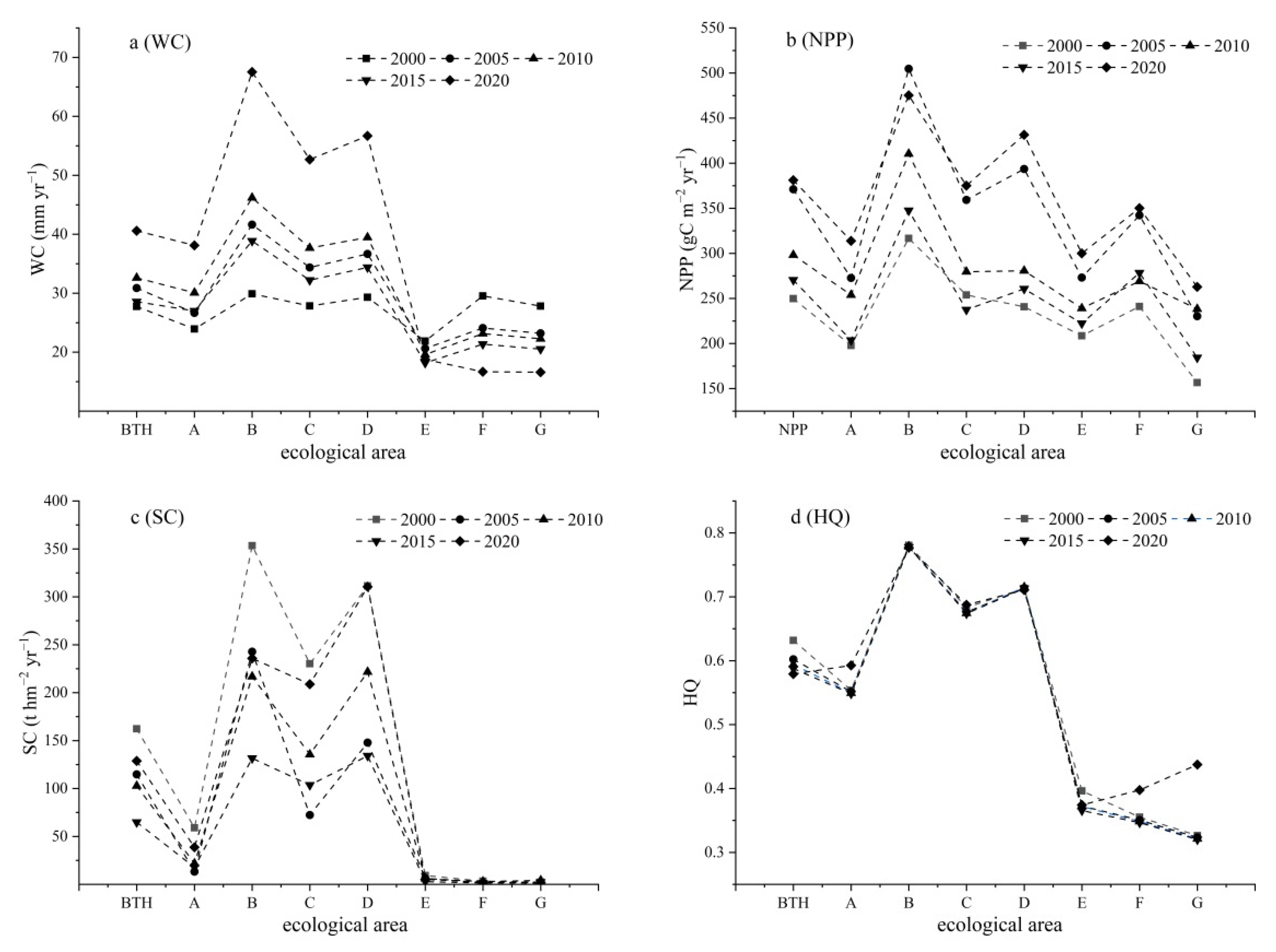
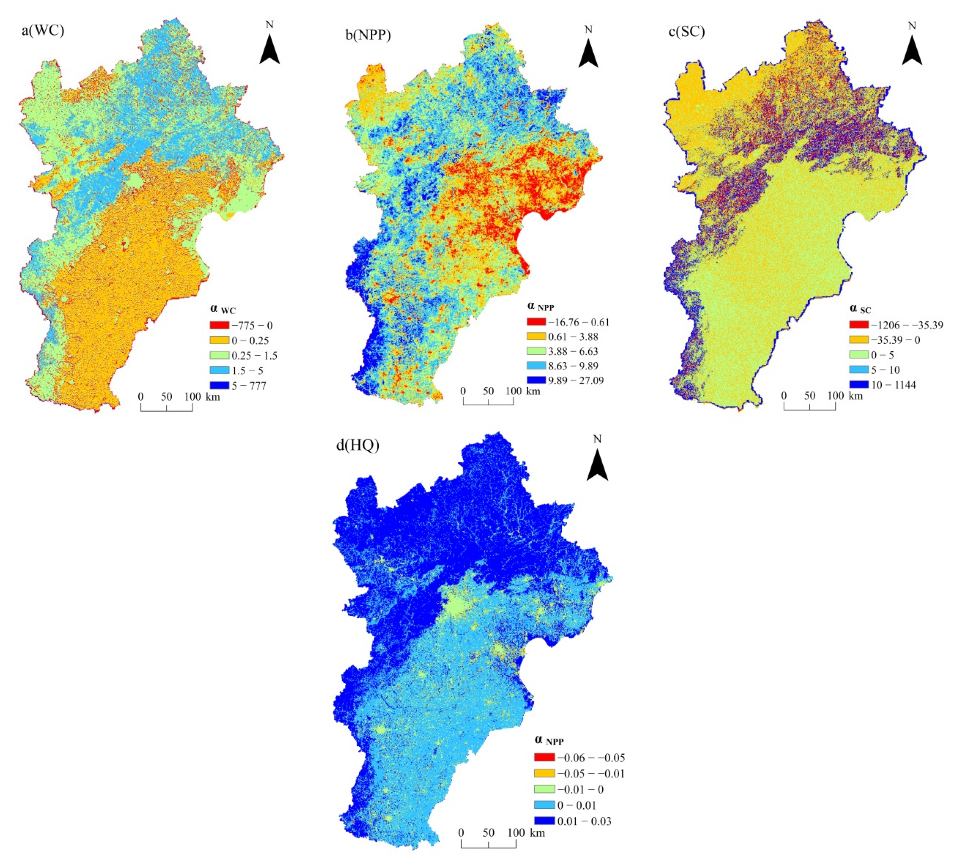
3.1. Spatio-Temporal Characteristic of Ecosystem Services in BTH

Compared with 27.76 mm in 2000, WC increased at the rate of 0.77 mm/year during 2000–2020 (Figure 2a); the maximum WC reached 40.59 mm in 2020. There was a significant spatial gap in WC among different ecological areas (Figure 3a). The mean value (43.78 mm) and increase rate (1.15 mm/year) of WC in Region B were much higher than those in other regions. In recent 20 years, WC only in Region F and G showed a downward trend, with a rate of 0.13 mm/year and 0.1 mm/a, respectively. The development of agriculture and continuous expansion of cultivated land in North China Plain led to the increase of regional water resource consumption and poor water conservation capacity.
NPP showed an increasing trend, with the rate of 5.28 gC·m−2·year−1. The lowest NPP was 249.79 gC·m−2·year−1 in 2000 and the highest was 249.79 gC·m−2·year−1 in 2020 (Figure 2b). In the last 20 years, NPP in Regions B, D, and F of Yanshan-Taihang Mountain and North China Plain was 308.72~428.66 gC·m−2·year−1) (Figure 3b), which was much higher than that in Bashang Plateau of Region A (254.01 gC·m−2·year−1). In addition, the increasing rate of NPP in Region C and D was up to 6.44 gC·m−2·year−1 and 8.11 gC·m−2·year−1, respectively, which was much higher than other regions. This was mainly affected by ecological projects, such as the policy of “Three-North Shelter Forest Program” and the program of Grain for Green, which made the productivity of plant communities in mountainous regions raise continuously and the high value area of NPP increase significantly.
From 2000 to 2020, SC decreased from 162.25 t·hm−2 year−1 to 128.8 t·hm−2 year−1 and reduced by 20.62% at a rate of −0.893 t·hm−2 year−1 (Figure 2c). The SC variation was different among all ecological regions (Figure 3c). Except for the slight increase rate of 0.02 t·hm−2 year−1 in Region G, the other six ecological regions showed a decreasing trend. Among them, Northern of Hebei and Yanshan Mountains (Region B) and Bashang Plateau (Region A) demonstrated the most significant decreasing trend, with a rate of 2.09 and 0.91 t·hm−2 year−1, respectively, which was related to continuous expansion of regional farmland and continuous reduction of forestland with strong root interception ability. In addition, construction land in these areas also expanded, resulting in obvious attenuation of regional soil conservation capacity.
The HQ reduced from 0.631 to 0.577 during 2000–2020, with a decrease rate of 8.32% (Figure 2d). Spatially, the decreasing rate of HQ in North China Plain and coastal regions (Regions E, F, and G), greatly affected by human activities, showed the greatest decrease. The expansion of cities such as Beijing and Tianjin and the construction of new areas such as Xiong’an occupied a large amount of surrounding ecological land, which damaged the natural ecosystem and led to a significant deterioration in habitat quality.

3.2. Analysis on the Driving Factor of Ecosystem Service Variation

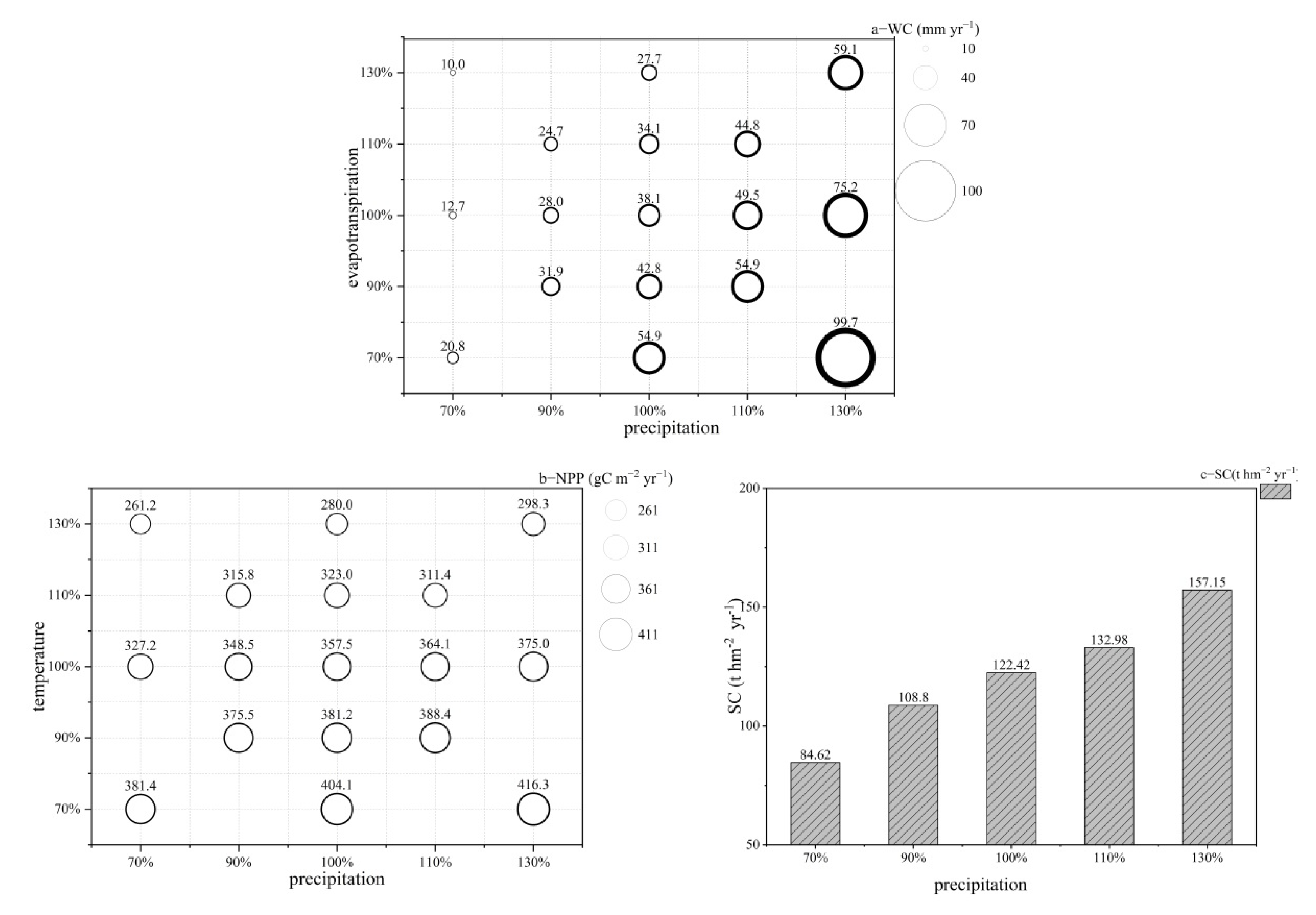
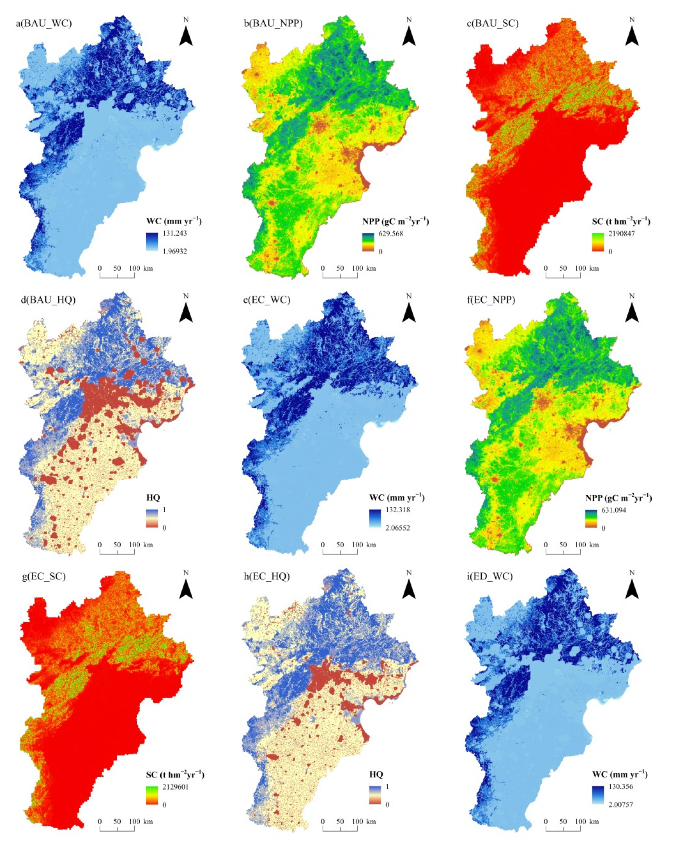
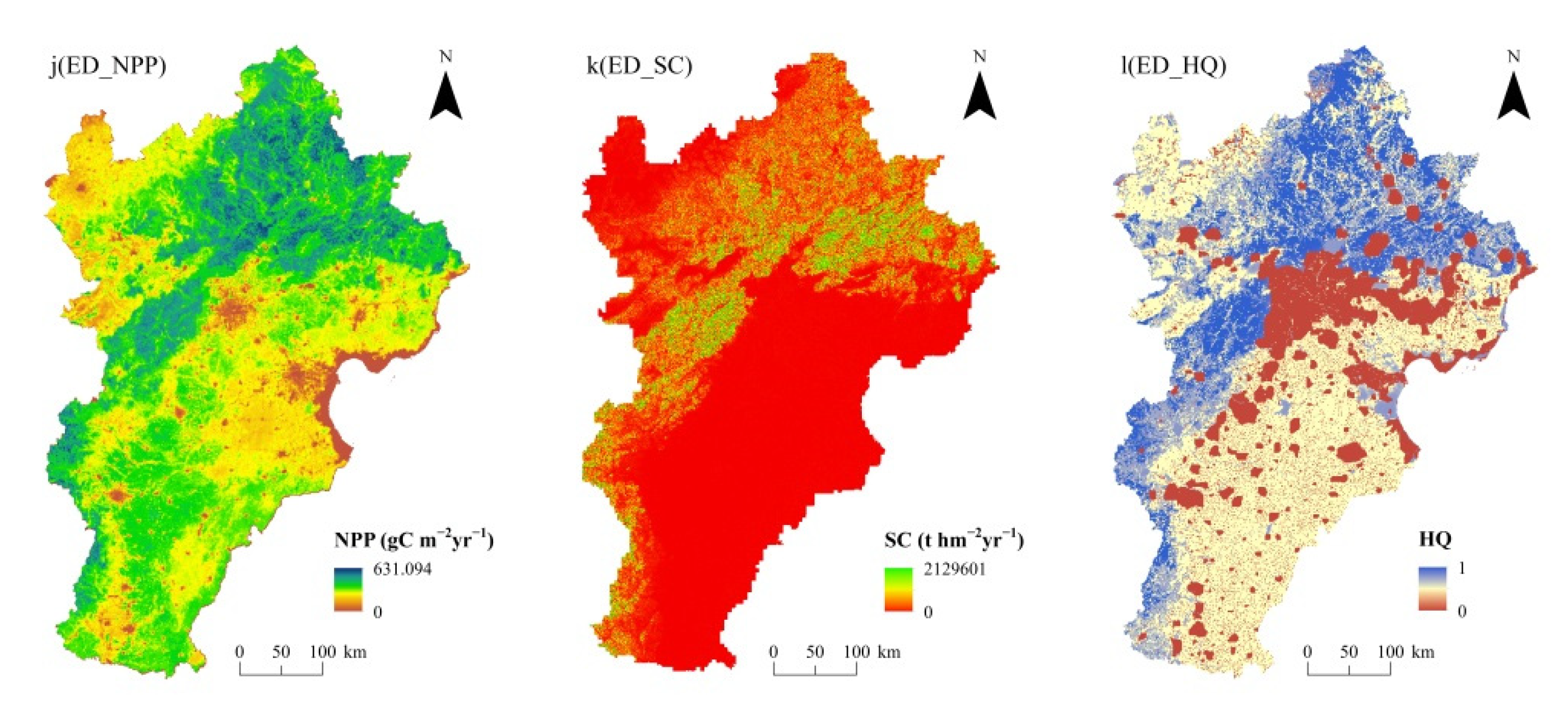
3.2.1. Impacts of Climate Change on Ecosystem Services

Table 5 showed the variation trends of temperature, precipitation, and potential evaporation in different ecological regions of BTH from 2000 to 2020. The regional annual average precipitation and temperature presented an increasing trend, with growth rates of 4.06 mm/year and 0.003 °C/year respectively; the annual average potential evaporation showed a decreasing trend with the linear change rate of −3.56 mm/year. On the whole, the climate in BTH tended to be warm and humid, but there were spatial differences in climate change among each ecological region. The central and southern parts of BTH showed a warming trend, while the northern part showed a weak cooling trend; the increasing trend of precipitation in plain area is significantly higher than that in mountainous area. The temperature rise and decreasing trend of potential evaporation in Region D was the most obvious, while the increase of precipitation was relatively small, which was caused by the strengthened fohn effect by the proximity of Taihang Mountain to the west. The obvious trend of warming and humidification in Region E lied in the accelerated expansion of urbanization in the past 20 years. The proportion of construction land in 2020 had reached 30%, the urban impervious surface area had surged, and urban heat island and wet island effects had been significantly strengthened.
To diminish the impact of climatic anomaly in special years, the average climate state during 2010–2020 was set as the baseline. One must quantitatively evaluate the responses of WC, SC, and NPP to variation of 30% and 10% in precipitation and potential evaporation (Figure 4). Under the condition of constant potential evaporation, WC would increase 97.16% or decrease 66.73% with precipitation increase (decrease) 30%, and WC would increase 49.48% or decrease 28.02% with precipitation increase (decrease) 10%. Under the condition of constant precipitation, 30% increase (decrease) in potential evaporation would result in 27.4% decrease or 43.9% increase in WC, and 10% increase (decrease) in potential evaporation would lead to 10.5% decrease or 12.2% increase in WC. It can be seen that precipitation has a greater impact on WC than potential evaporation, and the change amplitude of WC caused by precipitation increase (potential evaporation decrease) was greater than that caused by precipitation decrease (potential evaporation increase), and the drastic change of precipitation presented greater impact on change amplitude of WC. Precipitation was also the main climate factor affecting soil conservation, and there was a very significant positive linear correlation between precipitation and SC (r = 1, p < 0.01). SC increased (decreased) by 36.13 t·hm−2 for every 10% increase (decrease) of precipitation. In addition, under the condition of constant precipitation, a 30% increase (decrease) in temperature could lead to an NPP decrease of 21.68% or increase of 13.04% and a 10% increase (decrease) in temperature would result in a 9.64% decrease or 6.63% increase in NPP. Under the condition of constant temperature, a 30% increase (decrease) in precipitation could cause NPP to increase 4.8% or decrease 8.4% and a 10% increase (decrease) in precipitation would result in a 1.8% decrease or 2.5% increase of NPP. The influence of temperature and precipitation on NPP is nonlinear, which was similar to the relationship between climate factors and WC. Meanwhile, the influence of temperature was greater than precipitation, and the decline of NPP caused by temperature rise (precipitation decrease) was greater than that caused by temperature fall (precipitation increase).

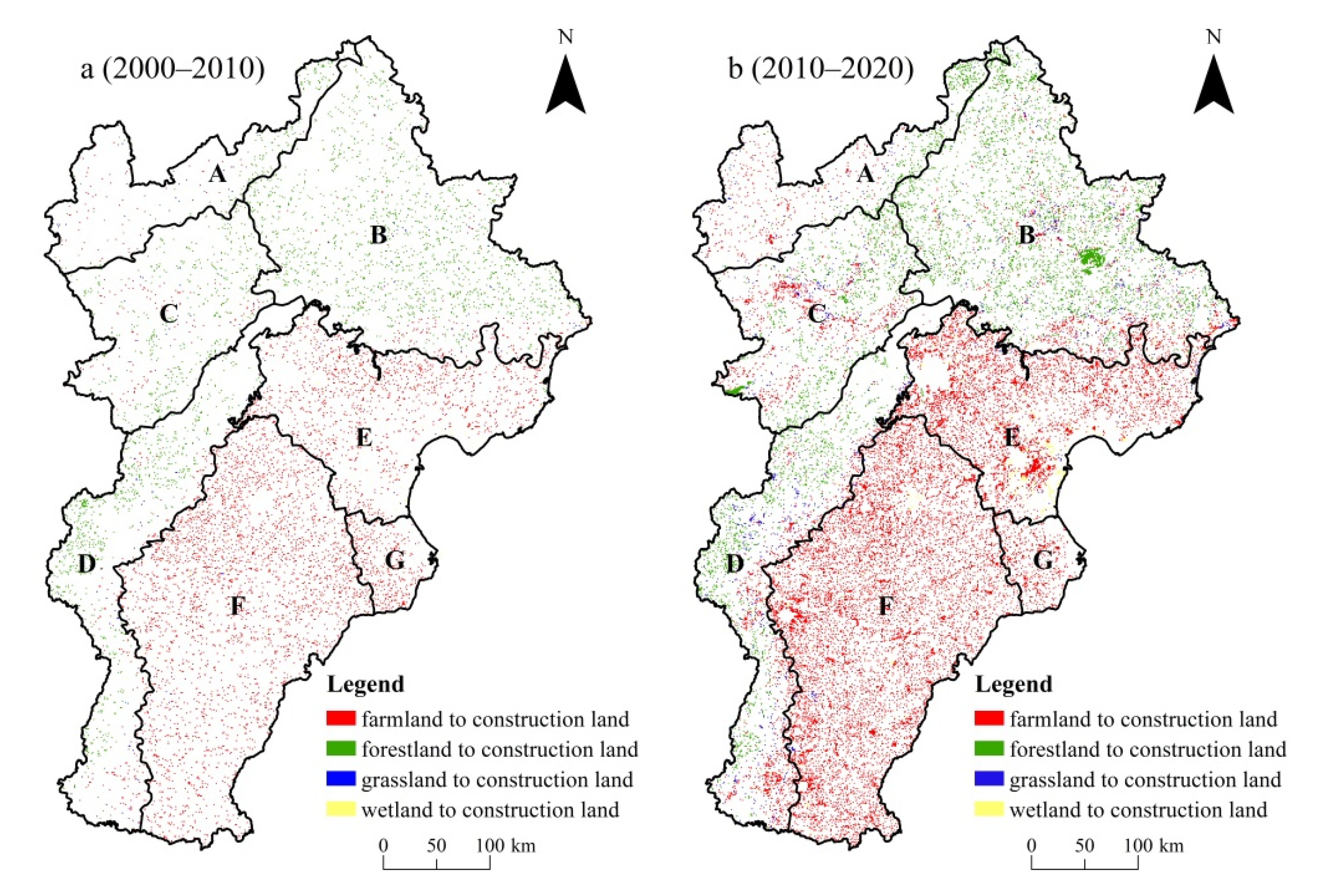
3.2.2. Impact of Land Use Change on Ecosystem Services

From 2000 to 2020, cultivated land, grassland, and unused land in BTH decreased, while construction land, forestland, and water area increased (Table 6). The most remarkable feature of land transfer was the transformation from cultivated land to construction land. In the past 20 years, cultivated land decreased by 9539 km2, while construction land increased by 9869 km2, and the net transformation area was up to 8614 km2. In addition, the increased forestland and water area were mainly artificial economic forests, ponds, reservoirs, and other artificial water bodies, which were mainly converted from farmland and have limited effect on the promotion of ES. The decreased grassland mainly transformed into construction land, which directly led to the shrinkage of ecological land. From the perspective of spatial variation of land transfer (Figure 5), the conversion of ecological land such as forestland and grassland to construction land mainly concentrated in Yanshan-Taihang mountain area, while the transformation of cultivated land to construction land mainly occurred in North China Plain. Meanwhile, the intensity of land use transfer in 2010s was much greater than that in 2000s, which was closely related to the large-scale urban expansion in BTH.
Figure 6 shows the variation of four kinds of ESs in BTH in 2030 under the scenarios of BAU, ED, and EC. The average WC in the base period (2010s) was 38.05 mm, and WC in 2030 under three scenarios was more than 50 mm. Especially in the ecological protection situation, WC reached 55.83 mm, with an increase of 46.7% compared with the 2010s. From the perspective of spatial variation, WC in Region B and D with high vegetation coverage increased the most, with the rate of 35.84 mm and 30.57 mm, respectively, in EC scenario. Under the BAU scenario, WC in Region F and G with great impact of human activities was slightly lower than that in the 2010s. Compared with the 2010s, NPP also showed an increasing trend in 2030 under the three scenarios, with an increase range of 5.16–5.94%, and land use change had little impact on NPP. Spatially, NPP of Region C and A in the northwest of BTH increased most significantly, with an increase of 12% and 17%, respectively, indicating that ecological engineering in Bashang Plateau and the upper reaches of Yongding River had achieved remarkable results. Compared with the base period, SC in 2030 would reduce around 2%, and simulation results under the three scenarios presented little difference. Region F and G distributed in North China Plain, with more than 99% of the areas having the slope of less than 2°, and the SC was extremely low (2.30–2.54 t·hm−2 year−1), which would increase slightly by 3.1–4.6% in 2030. In addition, SC in the other five ecological regions decreased, especially in Yanshan-Taihang Mountain area (Region C and D). Forestland and grassland greatly reduced and the SC decreased significantly, with a rate of 4.6–5.4 t·hm−2 year−1 (1.8–3.2%) under the three scenarios. The HQ in 2030 is 2.6–11.5% lower than that in 2010s under the three scenarios, and the ecological environment is seriously degraded. As a direct reflection of the transformation between ecological land and construction land, HQ is significantly affected by human activities. In Region E, where urbanization degree was the highest, construction land accounted for more than 50%, and HQ decreased significantly, with a reduced rate of 0.11 (30.89%), especially under the ED scenario. However, in Region F, where farmland accounted for more than 70%, even if ecological land (forest land and grassland) was less than 10%, the HQ still increased by 13.49% (0.05) due to the reduction of construction land under the EC scenario.

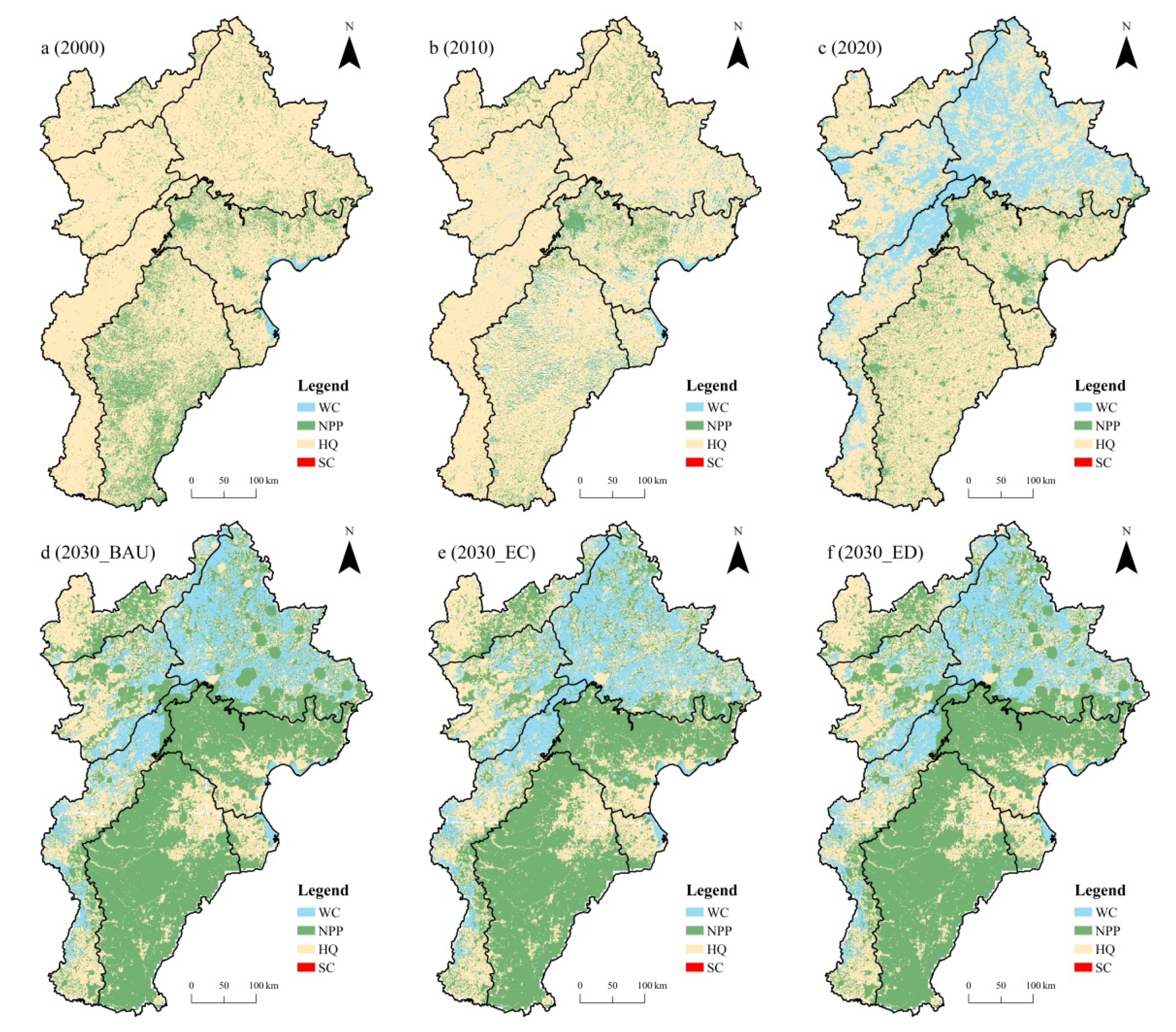
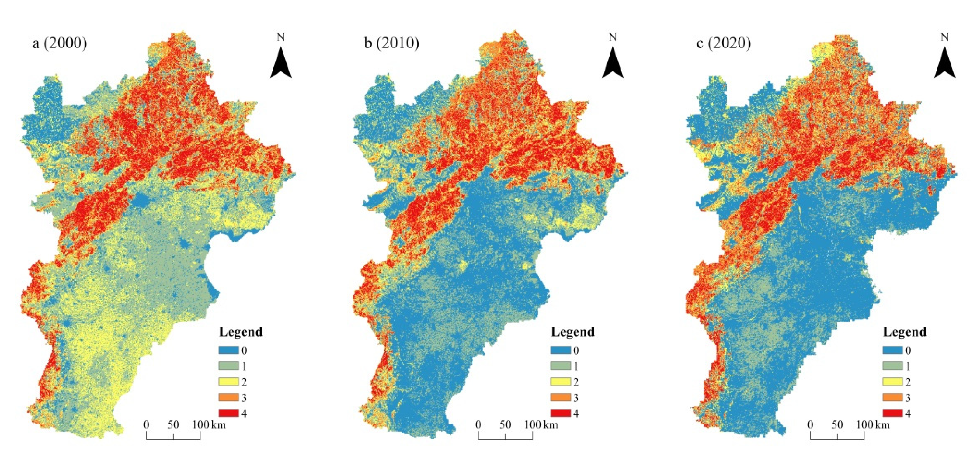
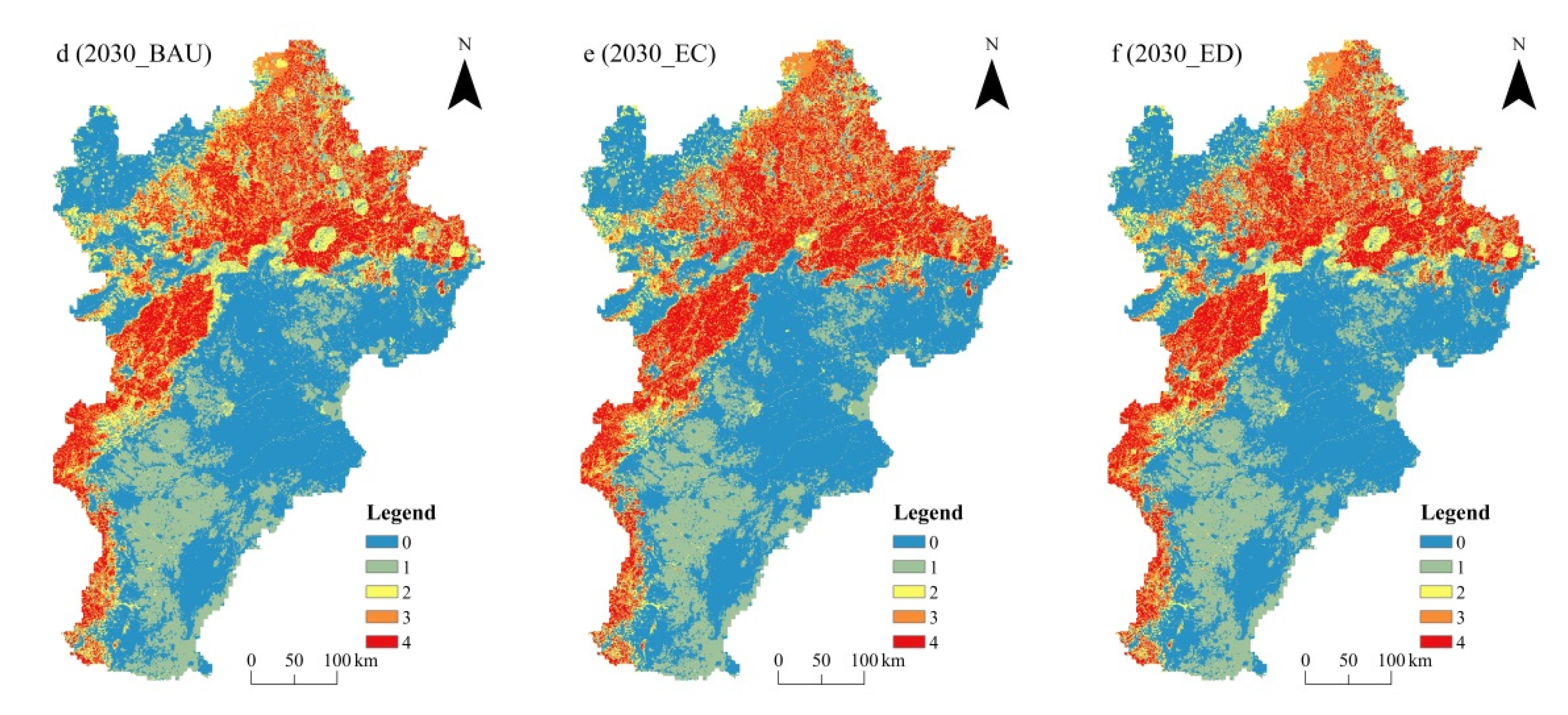
3.3. Identification of Ecosystem Services Hotspots from 2000 to 2030

The spatial distribution of the primary ecosystem hotspots in BTH is shown in Figure 7. WC and NPP have gradually become the primary ecosystem service of BTH from 2000 to 2020. The primary hotspots of WC gradually spread from coastal areas (Region G) to mountainous areas (Regions B, C, and D). NPP hotspots widely distributed in North China Plain (Regions E and F) in 2030, and their area increased by about 1.06 times in 30 years. At the same time, the proportion of HQ hotspots decreased significantly and was expected to shrink by about 65%. The SC hotspots were very small: less than 0.001% of the total area. In the future, NPP will become the biggest contributor for the ecological importance of BTH, and WC is the fastest-growing ecosystem service function at present. Therefore, more attention should be paid to the protection and development of WC and NPP in future ecological protection policies of BTH.
According to the statistical results of multiple service hotspots (Figure 8, Table 7), the area of Class 0 service hotspots accounted for the largest proportion (38~41%), and the area with Class 2 service hotspots accounted for a relatively small proportion (8~11%) during 2000–2030. There were significant differences in distribution of ecosystem service classes among different ecological regions. The ecosystem service of North China Plain (Regions E, F, and G) was poor, and Class 0 and Class 1 service hotspots were mainly distributed in this region (Supplementary Information, Table S2). The Class 0 hotspots area always exceeded 50%, and the proportion even reached 95% in Region G. The ecosystem service became better in Bashang Plateau and mountainous areas, and Class 2, 3, and 4 service hotspots were widely distributed. The area of Class 4 service hotspots in Region B always accounted for more than 30%, while the area of Class 4 service hotspots in Region D kept increasing, which was expected to reach 33% by 2030 under the EC scenario. Therefore, the core areas of future ecological protection in BTH are mainly concentrated in the northern Bashang Plateau and Yanshan-Taihang Mountain and improving the existing ecological protection policies in this region is the key point of ecological protection. The ecosystem service of urban and agro-ecological regions is poor, the contradiction between urban expansion and ecosystem service protection is acute, and their coordinated development is the main task of ecological protection in this region.

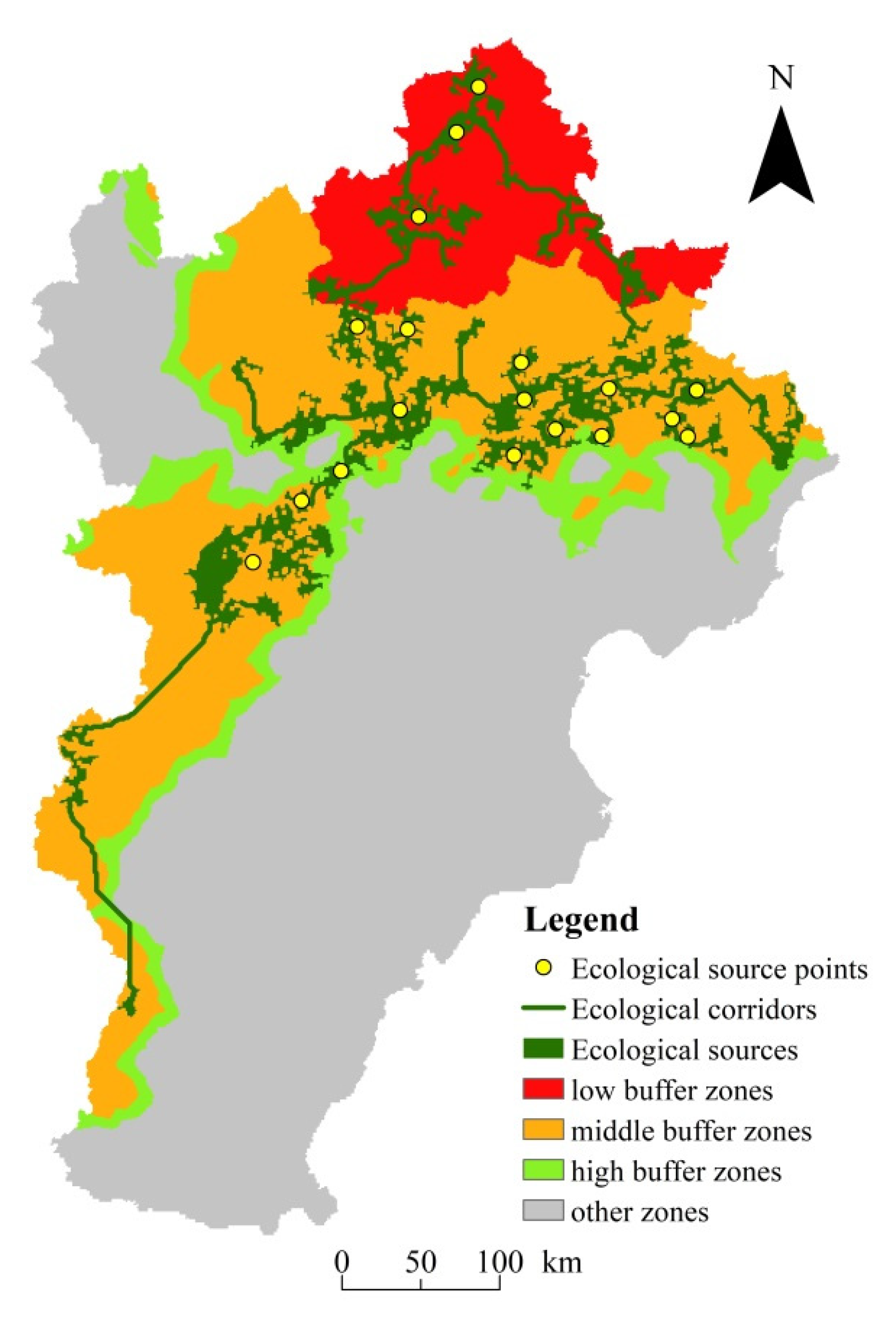
3.4. Identification of Ecological Security Pattern

Based on ESs, nature, economy, and society factors, the ecological security pattern of BTH was built (Figure 9). The ecological sources are the concentrated distribution area of ecological land, of which forestland accounted for 80.13%, followed by grassland (15.69%). The ecological corridor mainly covered the forestland (72.53%) and grassland (7.51%) of Yanshan-Taihang Mountain. There were eighteen important ecological nodes in the region, of which fifteen were distributed in the Yanshan Mountain. The ecological buffer zones were distributed in a belt along the ecological corridor, and the medium level buffer zone was the largest (60.36%), which was widely concentrated in Yanshan-Taihang mountain area. The high-level buffer zone was small (17.63%), which was banded around the middle level buffer. The low-level buffer zone (the last guarantee zone to ensure the safety of ecological source area) was mainly distributed in the north of Yanshan Mountain and the east of Bashang Plateau. Based on the distribution of various components of the ecological security pattern in BTH, the Northern Yanshan Mountain and the Intermountain basin in the upper reaches of Yongding River were important parts of the ecological security pattern. The key ecological corridors connected the ecological sources in a counterclockwise direction from northeast to southwest to form an ecological security network with a semi encirclement situation, which integrated the typical grassland area in the east of Bashang Plateau, the deciduous broad-leaved forest area in Yanshan Mountain, the forestland, farmland, and grassland of the Intermountain basin in the upper reaches of Yongding River, and the deciduous broad-leaved forest in the Taihang Mountains. These regions formed important ecological barriers in the agricultural areas of BTH and North China Plain due to high coverage of natural vegetation, low impact of human activities, and high ecosystem services.

4. Discussions

4.1. The Discussions on Driving Factor Analysis

At present, scenario simulation is widely used in analyzing the impact of land use change on ecosystem services, but it has hardly been used in analyzing the impact of climate change on ecosystem services. Previous studies mainly used multiple regression analysis or correlation analysis to explore the impact of climate on ecosystem services. They can only judge the dominant driving factors of ecosystem services through correlation or simply analyze the increase or decrease of ecosystem services caused by climate change. For example, precipitation is the main positive factor affecting water yield, but it is difficult to assess the variation magnitude of water yield caused by precipitation [63,64]. Indeed, the results obtained through climate change scenario simulation in this study not only fully demonstrate the main driving force of different ecosystem services but also further quantitatively analyze the difference of change rate between driving force and ESs. For example, temperature is the main factor leading to NPP change. Compared with temperature decrease, the change rate of NPP is more obvious when temperature increases.

4.2. The Discussions on Hotspots Analysis

In recent years, more and more studies have focused on classifying ecosystem services through hotspots analysis to explore the relationship between hotspot areas and urbanization. They believe that the research on this issue can determine the key areas of ecosystem service supply and explore the impact of land use change on ecosystem services [56,65,66]. However, previous studies mostly identified areas with high or low concentration of ecosystem service indicators through hotspots analysis (Getis-Ord Gi*) tool, which could not further identify the median-value area of ecosystem service level, resulting in the neglect of ecological protection [66,67,68]. This study comprehensively analyzes the ecosystem service hotspots in BTH from the perspective of multiple ecosystem service hotspots and primary ecosystem service hotspots and obtains five types of ecosystem service hotspots and two primary ecosystem services. Compared with other studies, the distribution trend of Class 4 hotspot is consistent with the other study [56], which is mainly distributed in the northern mountainous areas with high vegetation coverage, and the distribution of Class 0 and 1 hotspots basically coincides with other studies, mainly distributed in North China Plain. However, in our study the non-hotspots are further divided into Class 2 and 3 hotspots areas. Meanwhile, the primary ecosystem service hotspots analysis showed that NPP gradually took the place of WC and became the regional dominant ecosystem services. Therefore, in the process of formulating ecological security planning measures, we can refer to different levels of ecosystem service hotspots for ecological protection with different intensities and strengthen the key protection of WC and NPP, which will greatly improve the efficiency of ecological protection.

4.3. Linking Ecological Security Pattern and Planning Strategy in BTH

BTH is the largest and the most developed economic area in North China. The unreasonably rapid economic development at the cost of ecological loss in the early stage makes the region face problems such as water shortage, biodiversity loss, soil and water loss, ecological land degradation, and so on [69]. In recent years, more and more studies have realized the necessity and urgency of ensuring the ecological security pattern for the future development planning of BTH. However, previous studies on the ecological security pattern mostly focused on calculating the ecological environment carrying capacity from the administrative division scale, and reflecting the evolution of ecological security estimation through ecological security index, the evaluation results cannot reflect the impact of regional geographical environment on ecological security pattern [70,71]. Some other studies focus on the impact of the natural environment on the regional ecological security pattern, but the research mainly focuses on the construction of ecological security pattern in small regions, such as Xiong’an and the mountainous area in the north of Beijing [72,73,74]. Few studies have conducted a comprehensive analysis of the regional ecological security pattern of BTH. Therefore, based on the resistance surface in previous studies, this study constructs a set of ecological security patterns that can reflect regional natural and social factors by integrating natural factors, socio-economic factors, and ecosystem services [24].
A reasonable ecological security pattern can provide scientific guidance for optimizing the layout of ecological land. The northern low-level buffer zone of ecological security should reduce human intervention on ecology and is designated as an extremely important zone of ecological security. Developing economic activities on the basis of protection and restoration is the key issue in middle-level buffer zones, for example, forest parks can be properly developed. Other examples are taking the Beijing Winter Olympic Games as an opportunity to promote the construction of white snow and ice and green industries [75], preventing the construction of stadiums for the Winter Olympic Games from destroying the landform and landscape, reducing biodiversity, irrational use of water resources, environmental pollution, and other ecological problems [76,77,78]. High level buffer zone is an ideal area to protect regional ecological security. Moderate economic development activities will not block the ecological corridor and affect the ecological security pattern, so economic construction should be actively played to promote and protect ecological construction.

5. Conclusions

In summary, this study established a comprehensive ecosystem service analysis and regional security pattern evaluation system. The main conclusions are as follows: the inter-annual changes of WC and NPP showed an increasing trend from 2000 to 2020, and the increased rate in Yanshan-Taihang mountain area was significantly higher than that in the other area. Precipitation and temperature were the key climate factors controlling WC and NPP, respectively, and the impact of future land use change caused by policy orientation on WC cannot be ignored. At present, WC is the fastest-growing ecosystem service function in BTH, and NPP would become the greatest contributor to ecological importance in the future. Besides, SC was mainly affected by precipitation and showed an insignificant decreasing trend, while HQ was significantly reduced by the accelerated urbanization expansion, and the ecological environment tended to deteriorate in the past 20 years. Yanshan-Taihang mountain area has always been the key area of ecosystem service and the core region of ecological security in BTH. Due to high natural vegetation coverage and little effect by human activities, the ecological source was mainly distributed here, so the protection value here is pretty important. The result provides an effective direction and a scientific reference for the future territorial space planning and ecological restoration in BTH; the policy maker should reasonably control urban expansion in accordance with the ecological security pattern and pay attention to the development of areas with high NPP and WC.
However, there are still some problems to be improved in future research. The maximum light energy value required for CASA model simulation refers to the research results of light energy utilization calculation in China without better considering the special situation of the region. How to obtain the real data in the study area is the focus of future research. Meanwhile, our study only studies four supply services; more ecosystem services, such as supervision, culture, and supporting services, are not comprehensively selected to conduct a more comprehensive assessment of ecosystem services in BTH, which might be addressed in further studies.

Supplementary Materials

The following supporting information can be downloaded at: https://www.mdpi.com/article/10.3390/su14020699/s1, Supplementary Materials_A, Methods; Supplementary Materials_B: Table S2: The proportions of ecosystem service hotspots in in BTH and all ecological regions.

Author Contributions

Conceptualization, S.W.; formal analysis, J.W.; funding acquisition, S.W., Q.L. and J.W.; investigation, Q.L.; methodology, W.L.; writing—original draft, W.L.; writing—review and editing, W.L. All authors have read and agreed to the published version of the manuscript.

Funding

This research was funded by the National Key Research and Development Program of China (2020YFF0305905), the National Natural Science Foundation of China (41801034; 41801007), Shanxi philosophy and social science planning project (2020YY069, 2020YY070); Shanxi postgraduate education and teaching reform project (2021YJJG154).

Institutional Review Board Statement

Not applicable.

Informed Consent Statement

Not applicable.

Data Availability Statement

Data sharing not applicable. No new data were created or analyzed in this study. Data sharing is not applicable to this article.

Conflicts of Interest

The authors declare no conflict of interest.

References

  1. Zheng, H.; Wang, L.; Peng, W.; Zhang, C. Realizing the values of natural capital for inclusive, sustainable development: Informing China’s new ecological development strategy. Proc. Natl. Acad. Sci. USA 2019, 116, 8623–8628. [Google Scholar] [CrossRef] [PubMed] [Green Version]
  2. Millennium Ecosystem Assessment. Ecosystems and Human Well-Being: Synthesis; Island Press: Washington, DC, USA, 2005. [Google Scholar]
  3. La Notte, A.; D’Amato, D.; Mäkinen, H.; Maria, L.P.; Camino, L.; Benis, E.; Davide, G.; Neville, D.C. Ecosystem services classification: A systems ecology perspective of the cascade framework. Ecol. Indic. 2017, 74, 392–402. [Google Scholar] [CrossRef] [PubMed]
  4. Brito, I.; Goss, M.J.; Carvalho, M.D.; Chatagnier, O.; Tuinen, D. Impact of tillage system on arbuscular mycorrhiza fungal communities in the soil under Mediterranean conditions. Soil Till. Res. 2012, 12, 63–76. [Google Scholar] [CrossRef]
  5. Newbold, T.; Hudson, L.N.; Hill, S.L.L.; Contu, S.; Lysenko, I.; Senior, R.A.; Börger, L.; Bennett, D.J.; Choimes, A.; Collen, B.; et al. Global effects of land use on local terrestrial biodiversity. Nature 2015, 520, 45–50. [Google Scholar] [CrossRef] [Green Version]
  6. Nicu, C.T.; Roger, C.; Annelies, B.; Anabel, S.; Hermine, M.; Mirabela, M. Mainstreaming the nexus approach in climate services will enable coherent local and regional climate policies. Adv. Clim. Change Res. 2021, 12, 752–755. [Google Scholar] [CrossRef]
  7. IPBES; Willemen, L. Summary for policymakers of the assessment report on land degradation and restoration of the Intergovernmental Science-Policy Platform on Biodiversity and Ecosystem Services; IPBES Secretariat: Bonn, Germany, 2018; Available online: https://ipbes.net/assessment-reports/asia-pacific (accessed on 30 December 2020).
  8. Koppelmki, K.; Lamminen, M.; Helenius, J.; Schulte, R. Smart integration of food and bioenergy production delivers on multiple ecosystem services. Food Energy Secur. 2021, 10, 2048–3694. [Google Scholar] [CrossRef]
  9. Kumar, D.; Choudhury, M.; Rathore, A. Valuation of Ecosystem Services & Benefits of Son Beel Wetland in Assam, India: A Case Study of Natural Solutions to Climate Change & Water. SSRN Electron. J. 2020. [Google Scholar] [CrossRef]
  10. Wen, X.; Theau, J. Spatiotemporal analysis of water-related ecosystem services under ecological restoration scenarios: A case study in northern Shaanxi, China. Sci. Total Environ. 2020, 720, 137477.1–137477.13. [Google Scholar] [CrossRef]
  11. Nelson, E.; Mendoza, G.; Regetz, J.; Polasky, S.; Tallis, H.; Cameron, D.; Chan, K.M.; Daily, G.C.; Goldstein, J.; Kareiv, P.M.; et al. Modeling multiple ecosystem services, biodiversity conservation, commodity production, and tradeoffs at landscape scales. Front. Ecol. Environ. 2009, 7, 4–11. [Google Scholar] [CrossRef]
  12. Cabral, P.; Clément, F.; Levrel, H.; Chambolle, M.; Basque, D. Assessing the impact of land-cover changes on ecosystem services: A first step toward integrative planning in Bordeaux, France. Ecosyst. Serv. 2016, 22, 318–327. [Google Scholar] [CrossRef] [Green Version]
  13. Bai, Y.; Ochuodho, T.O.; Yang, J. Impact of land use and climate change on water-related ecosystem services in Kentucky, USA. Ecol. Indic. 2019, 102, 51–64. [Google Scholar] [CrossRef]
  14. Cardinale, B.J.; Duffy, J.E.; Gonzalez, A.; Hooper, D.U.; Perrings, C.; Venail, P.; Narwani, A.; Mace, G.M.; Tilman, D.; Wardle, D.; et al. Biodiversity loss and its impact on humanity. Nature 2012, 486, 59–67. [Google Scholar] [CrossRef] [PubMed]
  15. Hoyer, R.; Chang, H. Assessment of freshwater ecosystem services in the Tualatin and Yamhill basins under climate change and urbanization. Appl. Geogr. 2014, 53, 402–416. [Google Scholar] [CrossRef]
  16. Kusi, K.K.; Khattabi, A.; Mhammdi, N. Integrated assessment of ecosystem services in response to land use change and management activities in Morocco. Arab. Geosci. 2021, 14, 418. [Google Scholar] [CrossRef]
  17. Zhang, X.R.; Zhou, J.; Li, G.N.; Chen, C.; Li, M.M.; Luo, J.M. Spatial pattern reconstruction of regional habitat quality based on the simulation of land use changes from 1975 to 2010. J. Geogr. Sci. 2020, 30, 601–620. [Google Scholar] [CrossRef]
  18. Alexander, L.V.; Zhang, X.; Peterson, T.C.; Caesar, J.; Gleason, B.; Klein Tank, A.M.G.; Haylock, M.; Collins, D.; Trewin, B.; Rahimzadeh, F.; et al. Global Observed Changes in Daily Climate Extremes of Temperature and Precipitation. J. Geophys. Res. Atmos. 2006, 111, 1–22. [Google Scholar] [CrossRef] [Green Version]
  19. Thellmann, K.; Golbon, R.; Cotter, M.; Cadisch, G.; Asch, F. Assessing Hydrological Ecosystem Services in a Rubber-Dominated Watershed under Scenarios of Land Use and Climate Change. Forests 2019, 10, 176. [Google Scholar] [CrossRef] [Green Version]
  20. Liu, Z.; Yang, J.G.; Ma, L.H.; Ke, Z.M.; Hu, Y.M.; Yan, X.Y. Spatial-temporal trend of grassland net primary production and their driving factors in the Loess Plateau, China. Chin. J. Appl. Ecol. 2021, 32, 113–122. [Google Scholar] [CrossRef]
  21. Azam, M.; Khan, A.Q. Urbanization and environmental degradation:evidence from four SAARC countries-Bangladesh, India, Pakistan, and Sri Lanka. Environ. Prog. Sustain. 2016, 35, 823–832. [Google Scholar] [CrossRef]
  22. Fang, Y.S.; Zu, J.; Ai, D.; Chen, J.; Liang, Q.Y. Research on evaluation of the importance of ecological protection in Kunming city oriented to spatial planning. J. China Agric. Univ 2021, 26, 152–163. [Google Scholar] [CrossRef]
  23. Wu, J.G. Urban ecology and sustainability: The state-of-the-science and future directions. Landsc. Urban Plan. 2014, 125, 209–221. [Google Scholar] [CrossRef]
  24. Yu, K.J. Landscape ecological patterns in biological conservation. Acta Ecol. Sin. 1999, 19, 8–15. [Google Scholar] [CrossRef]
  25. Zhang, H.; Wang, A.Q.; Song, B.Y. Evaluation of Land Ecological Security in Dali City Based on OWA. Sci. Geogr. Sinica. 2017, 37, 1778–1784. [Google Scholar] [CrossRef]
  26. Tan, Q.H.; Zhang, J.T.; Zhou, X.S. Construction of Ecological Security Patterns Based on Minimum Cumulative Resistance Model in Nanjing City. Bull. Soil Water Conserv. 2020, 40282–40288, 40296, 40325. [Google Scholar] [CrossRef]
  27. Yu, C.L.; Liu, D.; Feng, R.; Tang, Q.; Guo, C.L. Construction of ecological security pattern in Northeast China based on MCR model. Acta Ecol. Sin. 2021, 41, 290–301. [Google Scholar] [CrossRef]
  28. Meng, J.J.; Wang, Y.; Wang, X.D. Construction of Landscape Ecological Security Pattern in Guiyang Based on MCR model. Resour. Environ. Yangtze Basin 2016, 25, 1052–1061. [Google Scholar] [CrossRef]
  29. Wang, Y.; Pan, J.H. Establishment of ecological security patterns based on ecosystem services value reconstruction in an arid inland basin: A case study of the Ganzhou District, Zhangye City, Gansu Province. Acta Ecol. Sin. 2019, 39, 3455–3467. [Google Scholar] [CrossRef]
  30. Liu, M.; Min, L.; Zhao, J.; Shen, Y.; Pei, H.; Zhang, H.; Li, Y. The Impact of Land Use Change on Water-Related Ecosystem Services in the Bashang Area of Hebei Province, China. Sustainability 2021, 13, 716. [Google Scholar] [CrossRef]
  31. Wang, B.S.; Chen, H.X.; Dong, Z.; Zhu, W.; Qiu, Q.Y.; Tang, L.N. Impact of land use change on the water conservation service of ecosystems in the urban agglomeration of the Golden Triangle of Southern Fujian, China, in 2030. Acta Ecol. Sin. 2020, 40, 484–498. [Google Scholar] [CrossRef]
  32. Liu, S.F.; Chen, J.M.; Guan, S.; Wang, H. Effect of Future Land Use Change on Water Conservation Function Based on InVEST Model—Taking Yangxi River Basin as an Example. J. Anhui Agric. Sci. 2020, 48, 67–70. [Google Scholar] [CrossRef]
  33. Wu, J.; Li, Y.H.; Huang, L.Y.; Lu, Z.M.; Yu, D.P.; Zhou, L.; Dai, L.M. Spatiotemporal variation of water yield and its driving factors in Northeast China. Chin. J. Ecol. 2017, 36, 3216–3223. [Google Scholar] [CrossRef]
  34. Ning, Y.Z.; Zhang, F.P.; Feng, Q.; Wei, Y.F.; Ding, J.B.; Zhang, Y. Temporal and spatial variation of water conservation service function in Qinling Mountain and its influencing factors. Chin. J. Ecol. 2020, 39, 3080–3091. [Google Scholar] [CrossRef]
  35. Wang, G.; Wang, L.; Wu, W. Recognition on regional ecological security definition and assessment system. Acta Ecol. Sin. 2007, 27, 1627–1637. [Google Scholar] [CrossRef]
  36. Li, P.F.; Liu, W.J.; Zhao, X.Y. The changes of atmospheric temperature, precipitation and potential evapotranspiration in Beijing—Tianjin—Hebei region in recent 50 years. J. Arid Land Resour. Environ. 2015, 29, 137–143. [Google Scholar] [CrossRef]
  37. Yan, S.J.; Wang, H.; Jiao, K.W. Spatiotemporal dynamic of NDVI in the Beijing-Tianjin-Hebei region based on MODIS data and quantitative attribution. J. Geo. Inf. Sci. 2019, 21, 767–780. [Google Scholar] [CrossRef]
  38. Zhai, Y.P.; Chen, Y.M.; Gao, J.X.; Song, T.; Feng, C.Y.; Nian, W. Division of Donor and Receptor Areas of Ecological Services of Water Conservation in Beijing-Tianjin-Hebei Region. Res. Environ. Sci. 2019, 32, 1099–1107. [Google Scholar] [CrossRef]
  39. Shi, M.; Wu, H.; Fan, X.; Jia, H.; Dong, T.; He, P.; Baqa, M.F.; Jiang, P. Trade-Offs and Synergies of Multiple Ecosystem Services for Different Land Use Scenarios in the Yili River Valley, China. Sustainability 2021, 13, 1577. [Google Scholar] [CrossRef]
  40. Haines, R.; Potschin, M. Revision of the Common International Classification for Ecosystem Services (CICES V5.1): A Policy Brief. One Ecosyst. 2018, 3, e27108. [Google Scholar] [CrossRef]
  41. Wong, C.P.; Jiang, B.; Kinzig, A.P.; Lee, K.N.; Ouyang, Z. Linking ecosystem characteristics to final ecosystem services for public policy. Ecol. Lett. 2015, 18, 108–118. [Google Scholar] [CrossRef] [PubMed] [Green Version]
  42. Li, D.; Sun, W.; Xia, F.; Yang, Y.; Xie, Y. Can Habitat Quality Index Measured Using the InVEST Model Explain Variations in Bird Diversity in an Urban Area? Sustainability 2021, 13, 5747. [Google Scholar] [CrossRef]
  43. Benra, F.; Frutos, A.D.; Gaglio, M.; Garretón, C.; Bonn, A. Mapping water ecosystem services: Evaluating InVEST model predictions in data scarce regions. Environ. Model. Softw. 2021, 104982. [Google Scholar] [CrossRef]
  44. Wang, L.X.; Li, M.M.; Qi, L.I.; Xu, X.L. Remote Sensing Estimation of NPP in Shaanxi Province based on CASA Model. J. West China. For. Sci. 2015. [Google Scholar] [CrossRef]
  45. Li, Y.Y.; Fan, J.H.; Liao, Y. Analysis of spatial and temporal differences in water conservation function in Zhangjiakou based on the InVEST model. Pratacult. Sci. 2020, 37, 1313–1324. [Google Scholar] [CrossRef]
  46. Zhou, B.; Yu, X.X.; Chen, L.H.; Zhang, Z.M.; Lv, X.Z.; Fan, M.R. Soil erosion simulation in mountain areas of Beijing based on InVEST Model. Res. Soil Water Conserv. 2010, 17, 9–13. [Google Scholar]
  47. Wischmeier, W.H.; Johnson, C.B.; Cross, B.V. Soil erodibility nomograph for farmland and construction sites. J. Soil Water Conserv. 1971, 26, 189–193. [Google Scholar] [CrossRef] [Green Version]
  48. Williams, J.R.; Jones, C.A.; Dyke, P.T. Modeling approach to determining the relationship between erosion and soil productivity. Trans. ASAE 1984, 27, 0129–0144. [Google Scholar] [CrossRef]
  49. Deng, Y.; Jiang, W.G.; Wang, W.J.; Lu, J.; Chen, K. Urban expansion led to the degradation of habitat quality in the Beijing-Tianjin-Hebei Area. Acta Ecol. Sin. 2018, 38, 4516–4525. [Google Scholar] [CrossRef]
  50. Shui, W.; Du, Y.; Wang, Y.N.; Yang, H.F.; Fu, Y.; Fan, B.X.; Huang, M.Y. Spatio-temporal dynamics and scenarios simulation of trade-offs between ecosystem services in Min Delta urban agglomeration. Acta Ecol. Sin. 2019, 39, 5188–5197. [Google Scholar] [CrossRef]
  51. Zhu, W.Q.; Pan, Y.Z.; He, H.; Yu, D.Y.; Hu, H.B. Simulation of maximum light use efficiency for some typical vegetation types in China. Chin. Sci. Bull. 2006, 51, 457–463. [Google Scholar] [CrossRef]
  52. Guan, D.J.; Gao, W.J.; Wateri, K. Land use change of Kitakyushu based on landscape ecology and Markov model. J. Geogr. Sci. 2008, 18, 455–468. [Google Scholar] [CrossRef]
  53. Zhou, T.J.; Ni, C.; Zheng, X. Study on the Impact of Landuse Pattern Changes on Habitat Based on Ca-Markov and InVEST Models—A Case Study of Shallow Mountainous Areas in Beijing. J. Chin. Landsc. Archit. 2020, 36, 139–144. [Google Scholar] [CrossRef]
  54. Dan, H.E.; Jin, F.J.; Zhou, J. The Changes of Land Use and Landscape Pattern Based on Logistic-CA-Markov Model—A Case Study of Beijing-Tianjin-Hebei Metropolitan Region. Sci. Geogr. Sin. 2011, 31, 903–910. [Google Scholar] [CrossRef]
  55. Dai, L.; Tang, H.; Zhang, Q.; Cui, F. The trade-off and synergistic relationship among ecosystem services:A case study in Duolun County, the agro-pastoral ecotone of Northern China. Acta Ecol. Sin. 2020, 40, 2863–2876. [Google Scholar] [CrossRef]
  56. Wang, J.L.; Zhou, W.Q.; Pickett, S.T.A.; Yu, W.J.; Li, W.F. A multiscale analysis of urbanization effects on ecosystem services supply in an urban megaregion. Sci. Total Environ. 2019, 662, 824–833. [Google Scholar] [CrossRef] [PubMed]
  57. Liu, J.L. Simulation and Temporal- Spatial Tradeoffs of Ecosystem Services: A Case Study in Beijing-Tianjin-Hebei Region. Beijing. Master’s Thesis, Peking University, Beijing, China, 2013. [Google Scholar]
  58. Wu, W.H.; Peng, J.; Liu, Y.X.; Hu, Y.N. Tradeoffs and synergies between ecosystem services in Ordos City. Prog. Geog. 2017, 36, 1571–1581. [Google Scholar] [CrossRef]
  59. Tang, P.; Wang, H. Analysis on the suitability of green sponge space in modern city based on MCR model. J. Nanjing For. Univ. 2019, 43, 116–122. [Google Scholar] [CrossRef]
  60. Wu, J.H.; Liu, S.Y.; Bai, S. Identification and optimization of ecological corridors in Shenmu city based on landscape ecological security. Arid. Land Res. 2021, 38, 1120–1127. [Google Scholar] [CrossRef]
  61. Xu, S.; Wang, P.; Kong, W.D. Mountainous Optimization of Ecological Security Pattern Based on MCR Model from the Perspective of Disaster Prevention: A Case Study of Beijing-Tianjin-Hebei Mountainous Area. J. Catastrophol. 2021, 36, 118–123. [Google Scholar] [CrossRef]
  62. Wang, Y.; He, C.; Liu, R.G.; Wu, H.B.; Chen, G.Q. Community structure of summer bird in Shapotou nature reserve, Ningxia. Acta Ecol. Sin. 2017, 37, 5531–5541. [Google Scholar] [CrossRef]
  63. Pan, M.; Chen, T.W.; Huang, L.; Cao, W. Spatial and temporal variations in ecosystem services and its driving factors analysis in Jing-Jin-Ji region. Acta Ecol. Sin. 2020, 40, 5151–5167. [Google Scholar] [CrossRef]
  64. Cui, F.; Wang, B.; Zhang, Q.; Tang, H.P.; Maeyer, P.D.; Hamdi, R.; Dai, L.W. Climate change versus land-use change—What affects the ecosystem services more in the forest-steppe ecotone? Sci. Total Environ. 2020, 759, 143525. [Google Scholar] [CrossRef]
  65. Li, G.; Fang, C.; Wang, S. Exploring spatiotemporal changes in ecosystem-service values and hotspots in China. Sci. Total Environ 2016, 545–546, 609–620. [Google Scholar] [CrossRef]
  66. Wang, B.; Zhao, J.; Hu, X.F. Spatial pattern analysis of ecosystem services based on InVEST in Heihe River Basin. Chin. J. Ecol. 2016, 35, 2783–2792. [Google Scholar] [CrossRef]
  67. Guo, C.Y.; Gao, S.; Zhou, B.Y.; Gao, J.H. Effects of land use change on ecosystem service value in Funiu Mountain based upon a grid square. Acta Ecol. Sin. 2019, 39, 3482–3493. [Google Scholar] [CrossRef]
  68. Pan, H.H.; Wu, S.R.; Yang, Z.Q.; Wu, Z.T.; Zhang, H. Spatiotemporal pattern of hotspots (coldspots) of ecosystem services in coal fields of Shanxi Province. Arid Land Grogr. 2022. Available online: https://kns.cnki.net/kcms/detail/65.1103.x.20210604.0840.002.html (accessed on 30 December 2020).
  69. Li, S.X. The Dynamics of Ecosystem Services and Their Driving Factors in the Jing-Jin-Ji Region. Ph.D. Thesis, The Beijing Forestry University, Beijing, China, 2019. [Google Scholar]
  70. Wang, Z.B.; Liang, L.W.; Fang, C.L.; Zhuang, R.L. Study of the evolution and factors influencing ecological security of the Beijing-Tianjin-Hebei Urban Agglomeration. Acta Ecol. Sin. 2018, 38, 4132–4144. [Google Scholar] [CrossRef]
  71. Liu, J.; Li, W.; Zhou, W.; Han, L.; Qian, Y. Prediction of expansion pattern and impact on regional ecological security of Beijing-Tianjin-Hebei Metropolitan Region. Acta Ecol. Sin. 2018, 38, 1650–1660. [Google Scholar] [CrossRef]
  72. Peng, J.; Li, H.L.; Liu, Y.X.; Hu, Y.N.; Yang, Y. Identification and optimization of ecological security pattern in Xiong’an New Area. Acta Grogr. Sin. 2018, 73, 701–710. [Google Scholar] [CrossRef]
  73. Hu, Q.H.; Cong, N.; Yin, G.D. Ecological security pattern construction in typical ecological shelter zone: A case study of Chengde. Chin. J. Ecol. 2021, 40, 2914–2926. [Google Scholar] [CrossRef]
  74. Li, C.; Zhang, X.; Xu, Y.; Wang, X.; Hao, F.H.; Yu, S.J. Study on ecological security under the influence of human activities in the ecological barrier zone in Beijing-Tianjin-Hebei region. China Environ. Sci. 2021, 41, 3324–3332. [Google Scholar]
  75. Zhou, B. Research on the Green Development Strategy of Northern Beijing Under the Background of 2022 Winter Olympic Games. Chi. J. Environ. Manag. 2018, 10, 121–125, 140. [Google Scholar] [CrossRef]
  76. Prudnikova, N. Environmental Problems and unintended consequences of the Winter Olympic Games: A case study of Sochi 2014. J. Policy Res. Tour. Leis. Events 2012, 4, 211–214. [Google Scholar] [CrossRef]
  77. Scalenghe, R.; Fasciani, G. Soil Heavy Metals Patterns in the Torino Olympic Winter Games Venue (E.U.). Soil. Sediment Contam. 2008, 17, 205–220. [Google Scholar] [CrossRef] [Green Version]
  78. Sobol, A.L. No medals for Sochi: Why the environment earned last place at the 2014 Winter Olympic Games, and how host cities can score a “green” medal in the future. Villanova Environ. Law J. 2015, 26, 169–192. [Google Scholar]
Figure 1. The ecological regionalization of BTH region (A) Bashang Plateau grassland and agro-ecological region; (B) Northern Hebei and Yanshan Mountain deciduous broad-leaved forest ecological region; (C) Forest agriculture and grass ecological region in the mountain basin of the upper reaches of Yongding River; (D) Taihang Mountain deciduous broad-leaved forest ecological region; (E) Beijing-Tianjin-Xiongan suburban agro-ecological region; (F) Central South Hebei plain agro-ecological region; (G) Yundong Binhai plain agro-ecological region.
Sustainability 14 00699 g001
Figure 2. Temporal changes of ecosystem service in BTH and all ecological regions. (a) WC, (b) (NPP), (c) SC, (d) HQ.
Sustainability 14 00699 g002
Figure 3. Spatial distribution of ecosystem service change rate from 2000 to 2020 in BTH (WC (a), NPP (b), SC (c), and HQ (d)), α represents the change rate of four ecosystem services, which is classified based on the natural partition point method. Red represents the very low change rate, yellow represents the low change rate, green represents the medium change rate, blue represents the fast change rate, and dark blue represents the very fast change rate.
Sustainability 14 00699 g003
Figure 4. Impact of climate factors on ESs.
Sustainability 14 00699 g004
Figure 5. Spatial transition of land use during 2000–2010 (a) and 2010–2020 (b). (A) Bashang Plateau grassland and agro-ecological region; (B) Northern Hebei and Yanshan Mountain deciduous broad-leaved forest ecological region; (C) Forest agriculture and grass ecological region in the mountain basin of the upper reaches of Yongding River; (D) Taihang Mountain deciduous broad-leaved forest ecological region; (E) Beijing-Tianjin-Xiongan suburban agro-ecological region; (F) Central South Hebei plain agro-ecological region; (G) Yundong Binhai plain agro-ecological region.
Sustainability 14 00699 g005
Figure 6. ESs variation of BTH in 2030 under three scenarios (WC (a), NPP (b), SC (c), and HQ (d) in BAU scenarios; WC (e), NPP (f), SC (g), and HQ (h) in ED scenarios; WC (i), NPP (j), SC (k), and HQ (l) in EC scenarios. Color from top to bottom represents the change of ecosystem services from high to low).
Sustainability 14 00699 g006aSustainability 14 00699 g006b
Figure 7. Spatial distribution of primary ecosystem services hotspots in BTH in 2000 (a), 2010 (b), 2020 (c), 2030_BAU (d), 2030_EC (e), 2030_ED (f).
Sustainability 14 00699 g007
Figure 8. Spatial distribution of multiple ecosystem services hotspots in BTH in 2000 (a), 2010 (b), 2020 (c), 2030_BAU (d), 2030_EC (e), 2030_ED (f).
Sustainability 14 00699 g008aSustainability 14 00699 g008b
Figure 9. Ecological security pattern of BTH.
Sustainability 14 00699 g009
Table 1. Datasets used in the study.
DatasetsInformationResolutionPeriodSources
Meteorological dataThe meteorological data are rasterized by KrigingRaster;
1000 m
2000–2020China Meteorological Data Service Centre (http://data.cma.cn/)
(accessed on 9 March 2021)
NDVIMODIS13Q1Raster;
250 m
2000–2020NASA (https://ladsweb.modaps.eosdis.nasa.gov/) (accessed on 3 September 2021)
Land UseChinese multi-period land use and land cover remote sensing monitoring datasetRaster;
100 m
2000\2005\2010\2015\2020Resource and Environment Science and Data Center (http://www.resdc.cn/)
(accessed on 15 June 2021)
SoilChina soil databaseVector; 1:1,000,000-The Nanjing Institute of soil research, CAS (http://www.issas.cas.cn/)
(accessed on 3 March 2021)
DEMSRTM DEMRaster;
90 m
2000Geospatial data cloud (http://www.gscloud.cn/)
(accessed on 3 September 2021)
RoadChinese road vector datasetVector; 1:1,000,0002019National catalogue service for geographic information (http://mulu.tianditu.gov.cn)
(accessed on 17 August 2021)
Water ResourcesWater Resources Bulletinstatistics2000–2020Haihe River water conservancy commission (http://www.hwcc.gov.cn/)
(accessed on 25 October 2021)
Table 2. Computational methods of parameters.
ESsModelParameter Setting and ProcessingLiterature Source
WCInVEST
(water yield)
Based on the simulation results of water yield using the InVEST Model, the WC can be calculated by combining the water production with the topographic index, soil saturated hydraulic conductivity, runoff velocity coefficient, and other parameters[45]
SCInVEST
(SDR)
Rainfall erosivity factor is calculated by Wischmeier’s monthly scale formula; Soil erodibility factor is calculated by soil erodibility estimation model; Vegetation and management factor C and soil and water conservation measure factor P are set by referring to relevant literature[46,47,48]
HQInVEST
(habitat quality)
The habitat threat sources include cultivated land, construction land, and traffic land, which are extracted from the land use data with a resolution of 100 m. The habitat threat sources and sensitivity parameters are set by referring to the relevant literature in Beijing, Tianjin, and Hebei[49]
NPPCASAThe monthly maximum light energy of different vegetation types refer to the research results on the calculation of the light energy utilization in China[50,51]
Table 3. The land requirement of three different scenarios in 2030/km2.
LUCC TypeBase Line Data in 2015Land Requirement in 2030
2030(BAU)2030(EC)2030(ED)
Farmland108,698.5794,931.55103,467.7894,632.20
Forestland45,112.0839,322.9144,196.1139,346.39
Grassland35,285.6630,151.5132,808.3630,216.79
Wetland6181.028170.678432.458311.21
Construction land20,710.1242,823.4727,275.6443,673.76
Unused land2012.542599.901819.661819.66
Table 4. Resistance coefficient and its weight of landscape ecological security pattern.
Resistance FactorWeightResistance Level and Coefficient
National Highway0.094<0.5 km90.5–1 km71–2 km5
2–5 km35–10 km1>100
Highway0.072<0.5 km90.5–1 km71–2 km5
2–5 km35–10 km1>100
Railway0.061<0.5 km90.5–1 km71–2 km5
2–5 km35–10 km1>100
DEM0.265<300 m1300–600 m3600–900 m5
900–1200 m7>1200 m9
Slop0.249<3°13–8°38–15°5
15–20°7>209
NDVI0.1330–0.290.2–0.470.4–0.65
0.6–0.73>0.71
Land Use0.126Farmland5Forest land3Grassland5
Wetland1Construction land9Unused land7
Table 5. Variation trend of climate factors in BTH and each ecological region from 2000 to 2020.
Ecological RegionTemperature/°C a−1Precipitation/mm a−1Potential Evaporation/mm a−1
A−0.0095.1404−3.5931
B−0.01563.8168−1.6437
C0.00481.83−4.3579
D0.02623.4299−8.1656
E0.01685.7148−5.3265
F0.00294.2436−2.6836
G0.00595.0842−2.572
BTH0.00284.0562−3.559
Table 6. Transition matrix of land use change during 2000–2020 (km2).
2020FarmlandForestlandGrasslandWetlandConstruction LandUnused LandTransfer_Out
2000
Farmland83,44048117042225015,23037229,705
Forestland385433,74067262668403211,718
Grassland7015701718,700471128720615,996
Wetland181534748518977444763867
Construction land661624736211176241518393
Unused land86674296149161440.21546
Transfer_in20,16512,49514,912425218,2631137
Table 7. Proportion of Class 0–4 ecosystem services hotspots in BTH/%.
2000201020202030_BAU2030_EC2030_ED
013.7838.6545.5345.5341.4341.21
133.2922.2915.1715.1721.2819.78
226.1511.7611.3611.369.298.14
312.5014.2814.9314.9311.9413.18
414.2813.0313.0113.0116.0717.70
Publisher’s Note: MDPI stays neutral with regard to jurisdictional claims in published maps and institutional affiliations.

