
Research on Route Deviation Transit Operation Scheduling—A Case Study in Suburb No. 5 Road of Harbin

Abstract
:1. Introduction
2. RDT Operation Dispatching Model
2.1. Model Assumptions
- (1)
- Assuming that the number of travel requests of passengers is not greater than the maximum load capacity of the vehicle, that is, there is no problem of denying travel requests of passengers due to overcrowded vehicles.
- (2)
- The study in this section adopts one-way driving, assuming that the vehicle passes only once at each station, and each station (except the first and last station) has only one incident route and one exit route.
- (3)
- It is assumed that passengers in the service area on the entire route will not change their travel modes due to changes in the operating mode, that is, the number of passengers will not decrease.
- (4)
- It is assumed that the driving speed of the vehicle is uniform and constant, and it is not affected by traffic control facilities such as traffic lights and external forces.
2.2. Modeling
- (1)
- Vehicle operating cost.
- (2)
- Passenger travel time cost.
- (3)
- Passenger walking and waiting time costs
3. Algorithm Optimization
3.1. Control Parameter
3.2. Algorithm Establishment
3.2.1. Problem Description
3.2.2. Feasibility
3.2.3. Cost Function
3.2.4. Search Domain
3.2.5. Insert Program
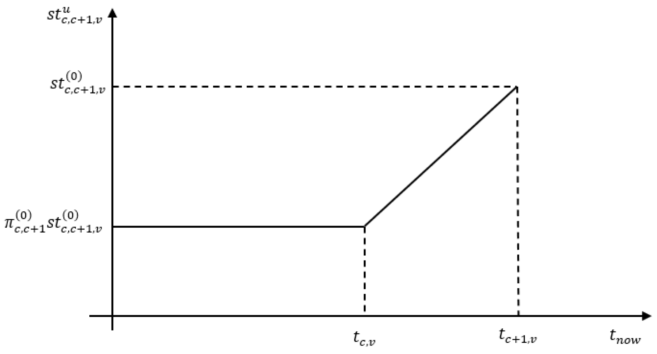
3.2.6. Correction of Relaxation Time
4. Case Analysis
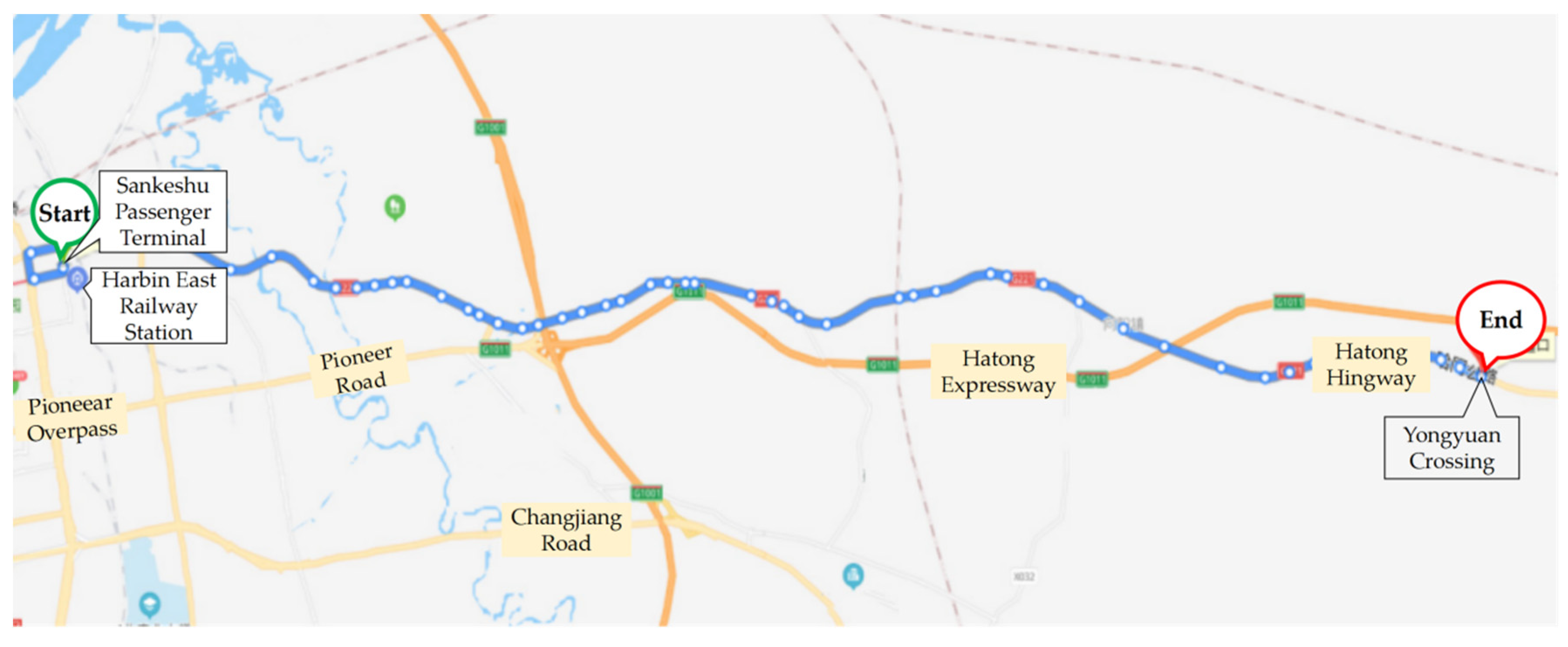
4.1. Route Selection
- (1)
- Passenger travel demand
- (2)
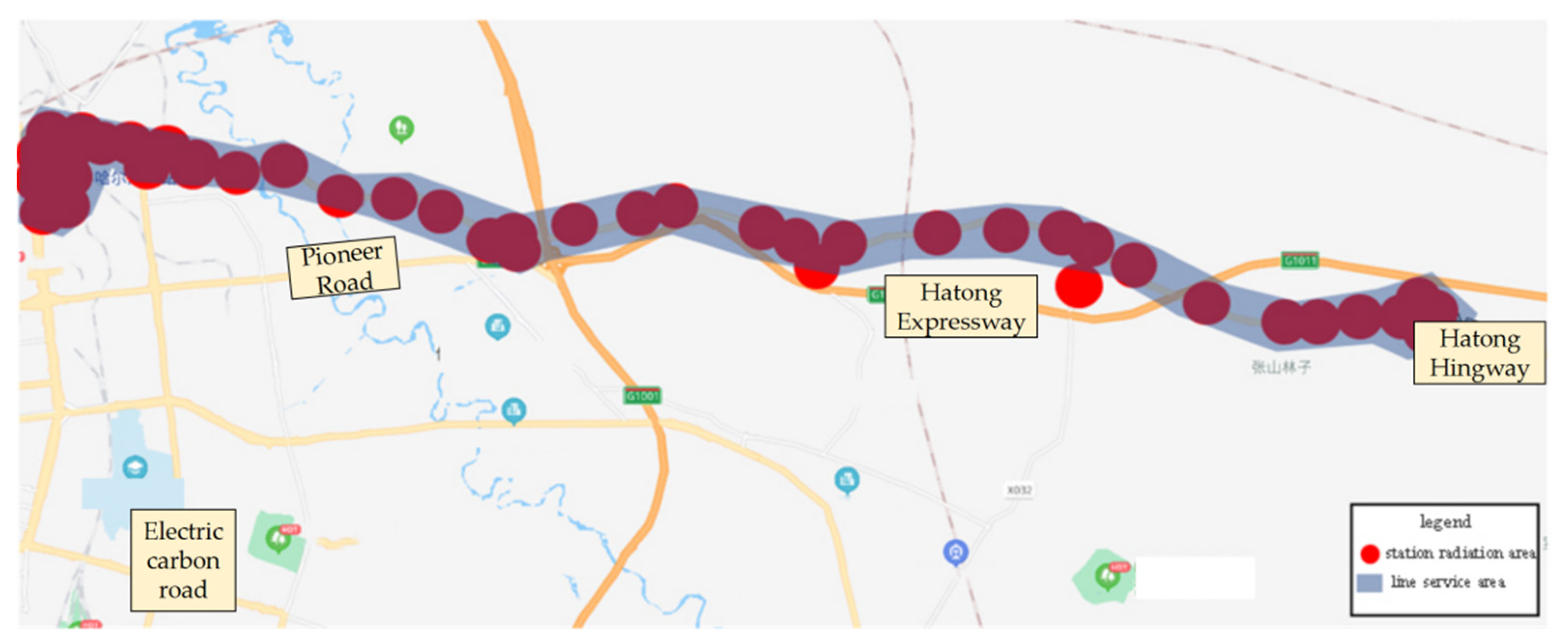
- Bus Station
- (3)
- Service area
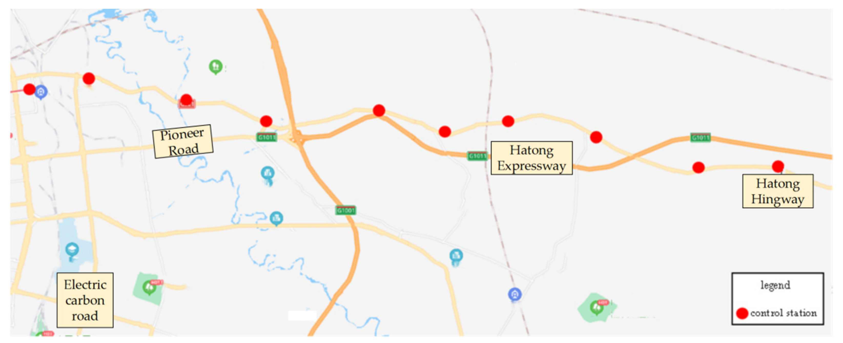
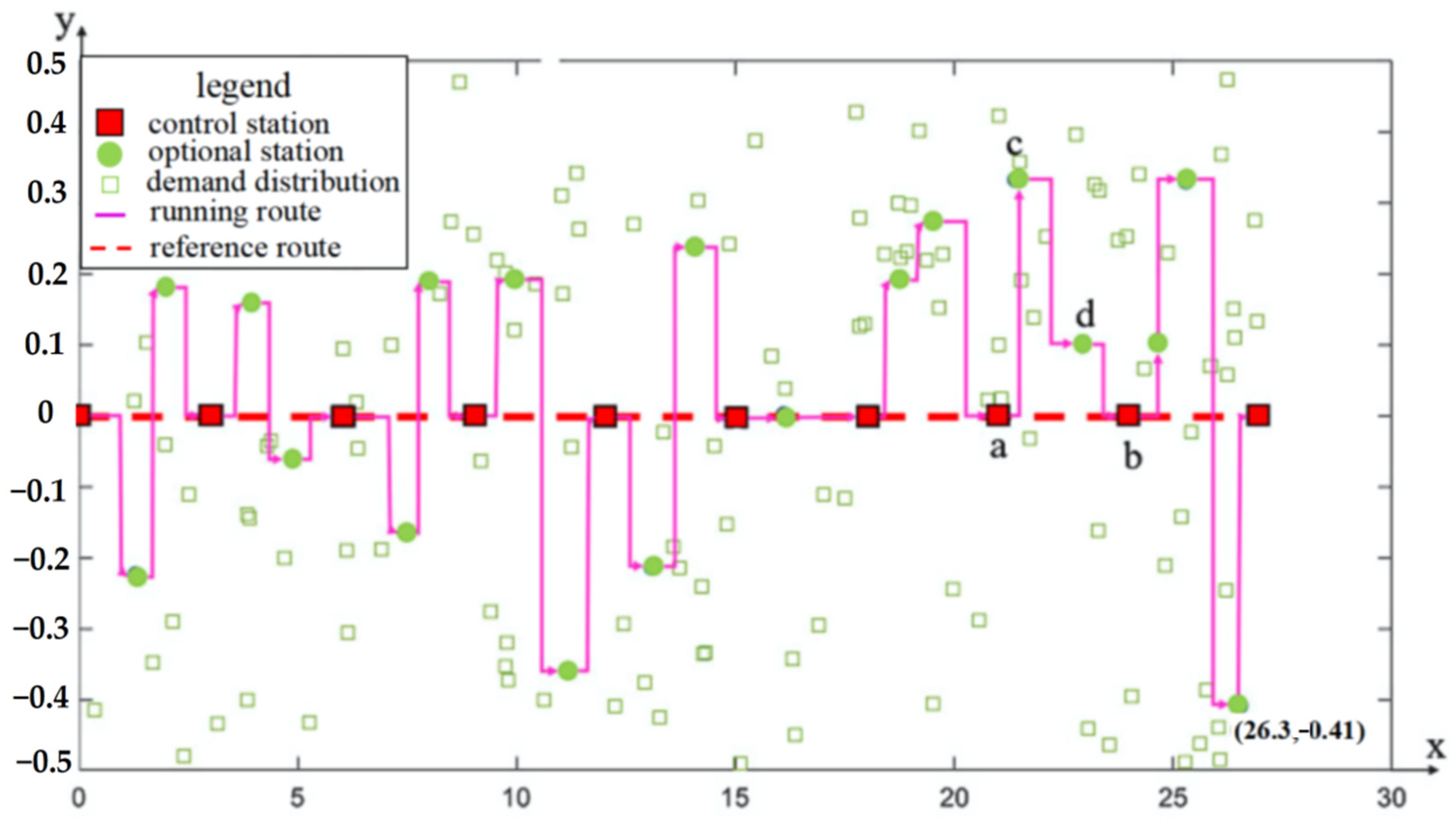
4.2. Site Selection of Bus Stops
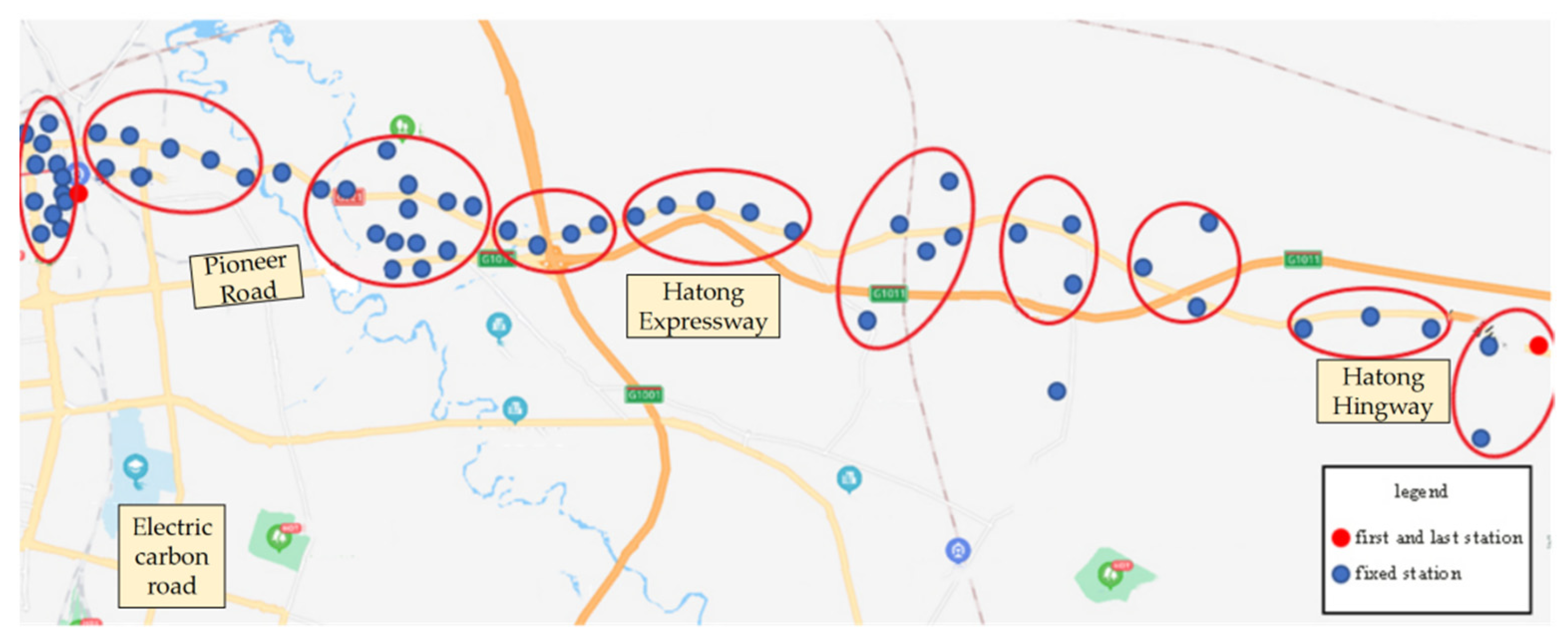
4.2.1. Control Station
4.2.2. Optional Station
- (1)
- The service area is in length and in width, and the service radius of the site is 500 m.
- (2)
- The passenger boarding time is set to 3.5 s per person, and the vehicle service time is 16 s.
- (3)
- The running speed of the vehicle is constantly set to , and the average walking speed of passengers is .
- (4)
- Passenger demand A is 30 people per hour, and passenger travel demand is uniform and random.
- (5)
- Passenger travel demand ratio PD:PND:NPD:NPND = 0.2:0.35:0.35:0.1.
- (6)
- The unit time value coefficient of each time cost , , ,
4.3. Scheduling Analysis
4.3.1. Simulation System Description
4.3.2. Simulation Results
5. Conclusions
Author Contributions
Funding
Institutional Review Board Statement
Informed Consent Statement
Conflicts of Interest
References
- Zheng, Y.; Li, W.; Feng, Q.; Cao, X. Flexible Transit Services: Choosing Between Route Deviation and Point Deviation Policy. In Proceedings of the Transportation Research Board 97th Annual Meeting, Washington DC, USA, 7–11 January 2018. [Google Scholar]
- Li, X.; Quadrifoglio, L. Optimal zone design for feeder transit services. Transp. Res. Rec. 2009, 2111, 100–108. [Google Scholar] [CrossRef] [Green Version]
- Francesco, B.; Federico, C.; Silvio, N. The integration of passenger and freight transport for first-last mile operations. Transp. Policy 2021, 100, 31–48. [Google Scholar]
- Silvio, N.; Giuseppe, P.; Francesco, B. How to evaluate and plan the freight-passengers first-last mile. Transp. Policy 2020, prepublish. [Google Scholar]
- Boarnet, M.G.; Giuliano, G.; Hou, Y.; Shin, E.J. First/last mile transit access as an equity planning issue. Transp. Res. Part A 2017, 103, 296–310. [Google Scholar] [CrossRef]
- Chandra, S.; Quadrifoglio, L. A model for estimating the optimal cycle length of demand responsive feeder transit services. Transp. Res. Part B 2013, 51, 1–16. [Google Scholar] [CrossRef]
- Jaw, J.J.; Odoni, A.R.; Psaraftis, H.N.; Wilson, N.H.M. A heuristic algorithm for the multi-vehicle advance request dial-a-ride problem with time windows. Transp. Res. Part B 1986, 20, 243–257. [Google Scholar] [CrossRef]
- Barr, R.S.; Golden, B.L.; Kelly, J.P.; Resende, M.G.C.; Stewart, W.R. Designing and reporting on computational experiments with heuristic methods. J. Heuristics 1995, 1, 9–32. [Google Scholar] [CrossRef] [Green Version]
- Campbell, A.M.; Savelsbergh, M. Efficient insertion heuristics for vehicle routing and scheduling problems. Transp. Sci. 2004, 38, 369–378. [Google Scholar] [CrossRef] [Green Version]
- Giuffrida, N.; Pira, M.L.; Inturri, G. On-Demand Flexible Transit in Fast-Growing Cities: The Case of Dubai. Sustainability 2020, 12, 4455. [Google Scholar] [CrossRef]
- National Academies of Sciences, Engineering, and Medicine, Transportation Research Board. Operational Experiences with Flexible Transit Service; National Academies Press: Washington, DC, USA, 2004; pp. 8–20. [Google Scholar]
- Madsen, O.B.G.; Ravn, H.F.; Rygaard, J.M. A heuristic algorithm for a dial-a-ride problem with time windows, multiple capacities and multiple objectives. Ann. Oper. Res. 1995, 60, 193–208. [Google Scholar] [CrossRef]
- Cunha, C.; Cortes, C.S. Sistema de apoio à decisão baseado em planilha eletrônica para otimização da programação de entrega de concreto pronto. J. Transp. Lit. 2014, 8, 125–158. [Google Scholar] [CrossRef] [Green Version]
- Drabikowski, M.; Nowakowski, S.; Tiuryn, J. Library of local descriptors models the core of proteins accurately. Proteins Struct. Funct. Bioinform. 2010, 69, 499–510. [Google Scholar] [CrossRef] [PubMed]
- Crainic, T.G.; Errico, F.; Malucelli, F.; Nonato, M. Designing the master schedule for demand-adaptive transit systems. Ann. Oper. Res. 2010, 194, 151–166. [Google Scholar] [CrossRef]
- Frei, C.; Hyland, M.; Mahmassani, H.S. Flexing service schedules: Assessing the potential for demand-adaptive hybrid transit via a stated preference approach. Transp. Res. Part C Emerg. Technol. 2017, 76, 71–89. [Google Scholar] [CrossRef]
- Huang, D.; Tong, W.; Wang, L. An Analytical Model for the Many-to-One Demand Responsive Transit Systems. Sustainability 2020, 12, 298. [Google Scholar] [CrossRef] [Green Version]
- Errico, F.; Crainic, T.G.; Malucelli, F. A survey on planning semi-flexible transit systems: Methodological issues and a unifying framework. Transp. Res. Part C Emerg. Technol. 2013, 36, 324–338. [Google Scholar] [CrossRef]
- Alrukaibi, F.; Alkheder, S. Optimization of bus stop stations in kuwait. Sustain. Cities Soc. 2018, 44, 726–738. [Google Scholar] [CrossRef]
- Quadrifoglio, L.; Dessouky, M.M.; Palmer, K. An insertion heuristic for scheduling Mobility Allowance Shuttle Transit (MAST) services. J. Sched. 2007, 10, 25–40. [Google Scholar] [CrossRef]
- Qiu, F. Two-stage model for flex-route transit scheduling. J. Southeast Univ. (Nat. Sci. Ed.) 2014, 44, 1078–1083. [Google Scholar]
- Zheng, Y.; Li, W.; Qiu, F. A slack arrival strategy to promote flex-route transit services. Transp. Res. Part C Emerg. Technol. 2018, 92, 442–455. [Google Scholar] [CrossRef]
- Zheng, Y.; Li, W.; Qiu, F. The benefits of introducing meeting points into flex-route transit services. Transp. Res. Part C Emerg. Technol. 2019, 106, 98–112. [Google Scholar] [CrossRef]
- Alshalalfah, B.; Shalaby, A.S. Sensitivity of Flex-Route Transit Service to Design and Schedule-Building Characteristics. In Proceedings of the Transportation Research Board Meeting, Washington, DC, USA, 9–13 January 2008. [Google Scholar]
- Zheng, Y.; Gao, L.; Li, W. Vehicle Routing and Scheduling of Flex-Route Transit under a Dynamic Operating Environment. Discret. Dyn. Nat. Soc. 2021, 202, 1–10. [Google Scholar] [CrossRef]
- Jiang, S.; Guan, W.; Yang, L. Feeder Bus Accessibility Modeling and Evaluation. Sustainability 2020, 12, 8942. [Google Scholar] [CrossRef]


| Station | Departure Times | ||||||||||||
|---|---|---|---|---|---|---|---|---|---|---|---|---|---|
| HES | 6:30 | 7:30 | 8:00 | 9:00 | 10:20 | 11:10 | 12:10 | 13:50 | 15:15 | 16:25 | 17:15 | 18:10 | |
| YC | 4:55 | 5:30 | 6:30 | 7:00 | 7:55 | 8:55 | 9:40 | 10:15 | 12:30 | 13:20 | 14:10 | 15:50 | 16:50 |
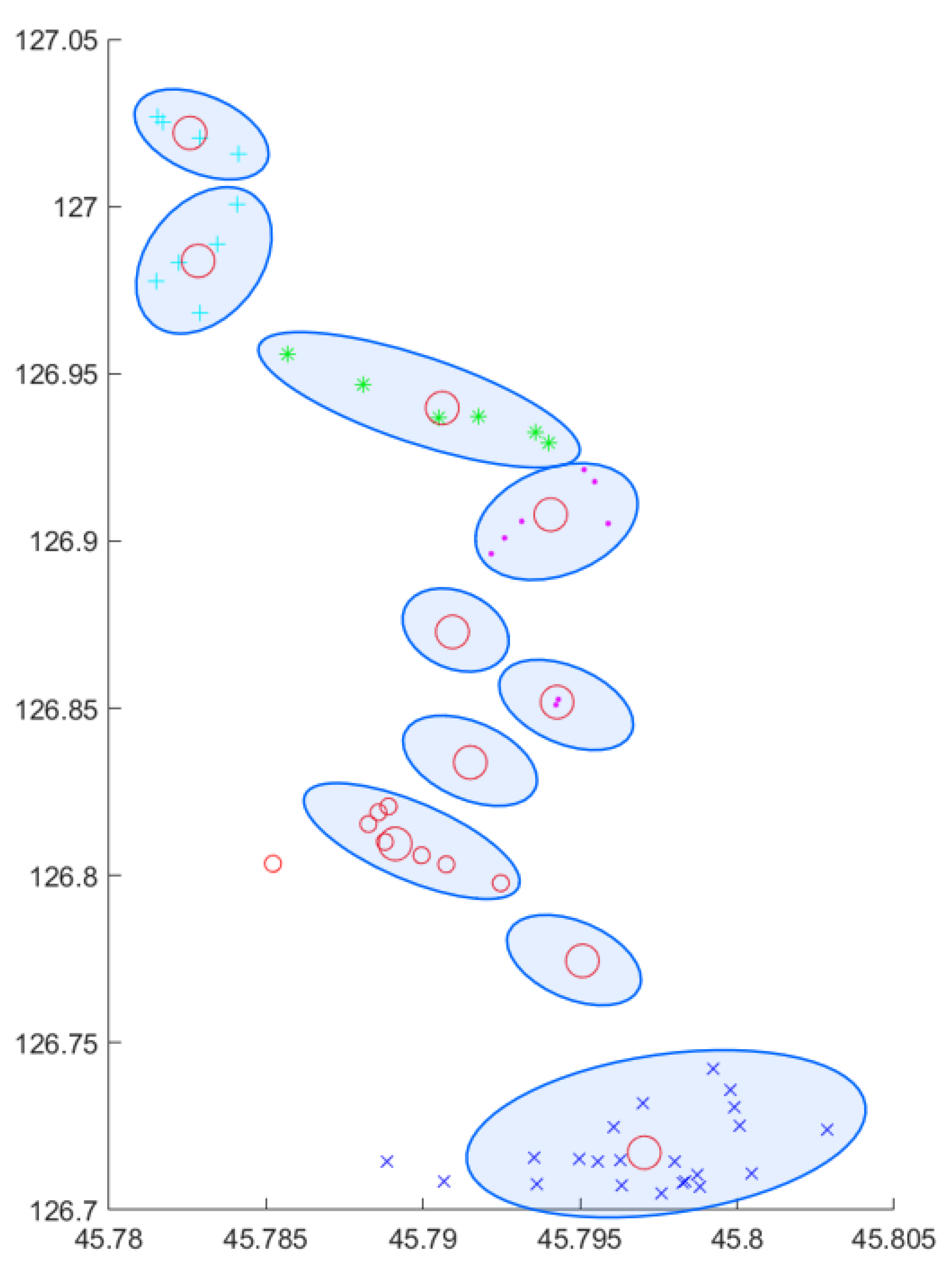
| Site Number | Longitude | Latitude | Site Number | Longitude | Latitude |
|---|---|---|---|---|---|
| 1 | 126.809448 | 45.789110 | 6 | 126.907870 | 45.794061 |
| 2 | 126.717145 | 45.797045 | 7 | 126.983718 | 45.782834 |
| 3 | 126.939738 | 45.790607 | 8 | 126.774467 | 45.795076 |
| 4 | 126.851818 | 45.794266 | 9 | 126.872808 | 45.790934 |
| 5 | 127.021983 | 45.782570 | 10 | 126.833767 | 45.791498 |
| Station Interval | (1,2) | (2,3) | (3,4) | (4,5) | (5,6) | (6,7) | (7,8) | (8,9) | (9,10) |
|---|---|---|---|---|---|---|---|---|---|
| Interval length | 2.1 | 3.8 | 2.9 | 3.9 | 2.2 | 2.1 | 3.3 | 3.7 | 3.0 |
| Number of potential stations | 2 | 4 | 3 | 4 | 2 | 2 | 3 | 4 | 3 |
| Site Number | Site Number | Site Number | |||
|---|---|---|---|---|---|
| 1 | 8.47 | 10 | 3.37 | 19 | 7.38 |
| 2 | 5.61 | 11 | 1.23 | 20 | 6.46 |
| 3 | 4.53 | 12 | 5.41 | 21 | 6.27 |
| 4 | 5.61 | 13 | 5.43 | 22 | 6.31 |
| 5 | 6.37 | 14 | 5.29 | 23 | 4.29 |
| 6 | 4.41 | 15 | 5.36 | 24 | 2.23 |
| 7 | 2.68 | 16 | 2.34 | 25 | 4.28 |
| 8 | 5.42 | 17 | 5.41 | 26 | 5.36 |
| 9 | 5.43 | 18 | 6.26 | 27 | 6.45 |
| Site Number | Longitude | Latitude | Site Number | Longitude | Latitude |
|---|---|---|---|---|---|
| 1 | 126.715664 | 45.793166 | 10 | 126.790044 | 45.796823 |
| 2 | 126.70855 | 45.794297 | 11 | 126.80783 | 45.786542 |
| 3 | 126.715844 | 45.799977 | 12 | 126.875527 | 45.791117 |
| 4 | 126.724252 | 45.797766 | 13 | 126.937114 | 45.786793 |
| 5 | 126.737259 | 45.796257 | 14 | 126.980736 | 45.775479 |
| 6 | 126.744805 | 45.80043 | 15 | 126.975418 | 45.77553 |
| 7 | 126.755369 | 45.798758 | 16 | 126.946601 | 45.789659 |
| 8 | 126.76579 | 45.794335 | 17 | 126.910525 | 45.799362 |
| 9 | 126.778438 | 45.792072 | 18 | 126.888031 | 45.780357 |
| System Indicators | RDT | Traditional Bus | |
|---|---|---|---|
| Case 1 | Case 2 | Case 3 | |
| 30.00 | 30.00 | 30.00 | |
| 27.10 | 29.00 | 20.00 | |
| 1.57 | 1.92 | 5.00 | |
| 5.74 | 6.83 | 7.50 | |
| (min) | 74.15 | 74.53 | 54.00 |
| 32.62 | 32.78 | 27.00 | |
| Per capita cost | 13.67 | 14.91 | 15.34 |
| RDT | Traditional Bus | |||||||
|---|---|---|---|---|---|---|---|---|
| 20 | 25 | 30 | 35 | 40 | 30 | 35 | 40 | |
| 26.54 | 27.36 | 27.10 | 26.80 | 27.20 | 22.56 | 22.64 | 22.61 | |
| 1.51 | 1.54 | 1.57 | 1.50 | 1.48 | 7.50 | 7.50 | 7.50 | |
| 5.62 | 5.73 | 5.74 | 5.82 | 5.85 | 7.69 | 7.48 | 7.55 | |
| (min) | 74.25 | 73.65 | 74.15 | 73.89 | 74.19 | 54.00 | 54.00 | 54.00 |
| 32.67 | 32.35 | 32.62 | 32.49 | 32.63 | 27.00 | 27.00 | 27.00 | |
| Per capita cost | 13.41 | 13.53 | 13.67 | 13.99 | 14.10 | 15.34 | 15.12 | 14.98 |
Publisher’s Note: MDPI stays neutral with regard to jurisdictional claims in published maps and institutional affiliations. |
© 2022 by the authors. Licensee MDPI, Basel, Switzerland. This article is an open access article distributed under the terms and conditions of the Creative Commons Attribution (CC BY) license (https://creativecommons.org/licenses/by/4.0/).
Share and Cite
Sun, X.; Liu, S. Research on Route Deviation Transit Operation Scheduling—A Case Study in Suburb No. 5 Road of Harbin. Sustainability 2022, 14, 633. https://doi.org/10.3390/su14020633
Sun X, Liu S. Research on Route Deviation Transit Operation Scheduling—A Case Study in Suburb No. 5 Road of Harbin. Sustainability. 2022; 14(2):633. https://doi.org/10.3390/su14020633
Chicago/Turabian StyleSun, Xianglong, and Sai Liu. 2022. "Research on Route Deviation Transit Operation Scheduling—A Case Study in Suburb No. 5 Road of Harbin" Sustainability 14, no. 2: 633. https://doi.org/10.3390/su14020633
APA StyleSun, X., & Liu, S. (2022). Research on Route Deviation Transit Operation Scheduling—A Case Study in Suburb No. 5 Road of Harbin. Sustainability, 14(2), 633. https://doi.org/10.3390/su14020633