Semi-Automatic Extraction of Geometric Elements of Curved Ramps from Google Earth Images

Abstract

Generating and updating roadway geometric elements from aerial images is necessary for multiple geospatial information system purposes, which have been addressed through various approaches. However, most existing methods cannot deal with challenges such as differently curved ramp characteristics, whereas measurements of geometric elements are still of low effectiveness and accuracy. This paper presents a new method for the semi-automatic extraction of horizontal parameters of curved highway ramps using Google Earth images. The proposed method first determines a road centerline manually using a graphics editor software; the file is then saved and processed with a program that analyzes and splits the centerline into its basic components. After that, the curvature analysis and linear fitting methods are integrated for automatic PC and PT determination. Finally, at the post-processing stage, the radii of the curves are computed automatically using the least-squares method. The proposed method was tested on four highway ramps and validated by comparison with the obtained design plans. Results show that the proposed method successfully detected the curves’ PC/PT and measured their radii with a high degree of accuracy.

1. Introduction

The purpose of constructing highway ramps is to allow traffic on highways to pass through the junction without interruption from other crossing traffic streams [1]. Generally, horizontal curves on highway ramps are designed to provide a smooth and safe transition between straight lines along the road trajectory, allowing the vehicle to safely pass a turn at a gradual rate instead of a sharp cut [2]. Unfortunately, as noticed by the Federal Highway Administration (FHWA) Office of Safety, a large number of serious vehicle crashes occur at interchange ramps of highways even though ramps only represent a small portion of the road network [3].

As a result, public studies have been undertaken to determine how the attributes of horizontal curves on the roads could be associated with the increase in crashes and how practical measures can reduce crash rates. Knowing the geometric elements of the horizontal curves and their location are critical in reducing crash rates.

Highway ramps are designed with curvature segments and tangents [4,5]. The lack of budget and site defects mean that variations from design standards can occur. The original design plan is often missing for ramps, making it difficult to assess safety performance. Therefore, a dedicated survey of the geometric elements of highway ramps (i.e., curve radius and curve length, point of curvature (PC), and point of tangent (PT)) after construction is essential for the analysis of safety-relevant issues to guarantee they meet design specifications [6,7]. Efficiently collecting such data helps the competent authorities to take corrective actions in case of design problems.

Traditional techniques used to collect information about horizontal curves, such as the plan sheet method [8], land survey method [9], and chord offset method, have required huge costs, labor, and time, which make them, in some cases, unpractical [10]. Thus, transportation authorities have been looking for an inexpensive, accurate, and time-efficient manner to obtain such information.

The emergence and potential use of high-resolution remote sensing images in a wide variety of applications, such as updating and preparing maps, have made object extraction, especially of buildings and roads, a new challenge in remote sensing [11]. Free online resources, including Google Earth (GE), have transformed the way design practitioners deal with spatial data [12,13], which can facilitate the description of the existing terrains. GE enables users to visualize any location on the Earth’s surface. Since 2005, when it was made accessible for public use, GE has been developed to be a widely used tool for academic research and other purposes [14].

This study proposes an accurate and semi-automatic method for extracting the parameters of horizontal curves on highway ramps from GE imagery, including the PC, PT, and curve radius. The proposed approach aims at facilitating the automatic extraction of the curves’ geometries to continuously update geospatial systems. Knowing the locations of horizontal curves and their parameters is essential to provide road users and autonomous vehicles with precise information in advance, while using the extracted data in safety prediction models to improve safety on curves.

2. Literature Review

Different technologies and approaches were used to extract roadway horizontal and vertical elements using various data sources. The data sources include field surveys [15], satellite imagery [16], AutoCAD (Automatic Computer-Aided Design,) digital map, GIS (geographic information system,) map, GPS (global positioning system) [17], LiDAR (light detection and ranging system) [18,19], and IMU (inertial measurement unit) [20]. However, field surveying methods using geomatic instruments, such as total stations, to obtain this data are time-consuming and costly [21]. GIS map, satellite imagery, and AutoCAD map provide a digital map for the extraction of the parameters of highway horizontal alignment, which has a complete road network data source and is low-cost in data collection. Depending on the mentioned data sources, the first stage is to extract road alignment geometric data (i.e., lane marking and road centerline) from the AutoCAD map, then identify curves and obtain geometric parameters using relevant approaches. Dong, H.; Easa, S.M. Li, J. [22] developed an algorithm based on Hough transform for curve extraction with satellite images and demonstrated the possibility of obtaining geometric features of a simple, spiral, and compound curves. However, due to the complexity of extracting unidentified elements of the spiral curve from aerial images, only symmetrical spirals have been considered in their research.

Rasdorf et al. [23] compared estimating elements of curves using curve finder (CF) and curvature extension (CE). CF uses GIS polylines as a tool to detect curve radius and length using GPS data. CF can identify curves while also determining their lengths and radius. CE is a plugin added into ArcGIS, which determines the length and radius of a horizontal curve. The two curve estimating tools were tested on two roads with different designs in North Carolina. CF detected 67% of road curves along the three paths. For 65% of the curves, CF detected a radius within 20% of that found using CE. The authors attribute the failure to obtain some curves due to their large radius.

Imran et al. [24] generated a technique of adding GPS data into the GIS platform to calculate the tangent, spiral length, and radius of the roadway curve. First, data points are subdivided into linear and non-linear depending on the variation in angle between consecutive data points. A PC and PT detection are obtained, and 75% of the tangent points are used to fit in a line for tangent segments. The Jacobian matrix method is then used to fit circles into curved segments. Additionally, using these types of surveying tools to collect curve data also limits the technique from being utilized on a large number of roads because of extended data collection time and the high cost.

The University of Wisconsin–Madison, based on GIS roadway maps, has established the CurveFinder tool that automatically identifies the geometric characteristics of horizontal curves. The CurveFinder tool extracts all horizontal curve attributes from GIS roadway maps, except for the super-elevation element, which can only be acquired by actual measurement; however, the algorithm could not distinguish between circular and spiral curves [25]. Researchers from Ireland and the United Kingdom proposed an approach to extract roadway geometric elements from digital maps using AutoCAD Civil 3D [26,27]. The authors used CAD commands to generate the centerline of the roadways based on the digitized road map in the CAD environment. Where the simple curves start and end can be located based on the reconstructed centerline. The geometric equations are used to estimate the curve length, radius, and angle. Their methods succeeded in extracting the sample curve, but more work is required when dealing with complex curves.

Xu and Wei [28] proposed a method based on the variation in bearing angles between consecutive vectors aligned along a roadway to detect the curve’s geometric features. They used a threshold for the variation in bearing that shows the beginning of a curve. When the start and end points of the curve are known (PC and PT), the curve length can be calculated and then applied to estimate the curve’s other features, including the deflection angle and radius. The authors noted successes in detection of up to 95% of the curves. However, their technique was not complete in recognizing spiral curves or extracting their geometric data.

An automatic approach was introduced to assess and detect the geometric information of horizontal curves based on LiDAR technology [4]. The proposed algorithm includes evaluating the differences in the azimuth between line segments and the road’s trajectory to identify horizontal curves on roadway segments. The outcomes show that the algorithm could determine all the curves on a roadway section; furthermore, the geometric attributes of those curves were obtained with reasonable accuracy. However, more work is required to distinguish simple curves from transition spiral curves.

In the curvature detection approaches, Tsai established a method based on vision technology to obtain roadway curvature data of horizontal curves from roadway images through multiple stages. Firstly, curve edges were detected using the image processing technique; secondly, roadway edge locations were mapped from the image domain to the real-world domain. Then, camera parameters were calibrated to remove the impact of capturing angles on image accuracy; finally, horizontal curves were measured [29].

As evident from the review, the previous methods using different data collection sources have shown their attempts to measure horizontal curve geometric elements, including simple, reverse, or spiral curves using an automated or semi-automatic manner. However, the automatic method is not widely used due to the limitation in extracting curves with different characteristics, whereas measurements of geometric elements of curved ramps are still of insufficient efficacy and accuracy. Moreover, some previous methods use costly software such as ArcGIS curve estimators to measure horizontal curve parameters.

In an attempt to address some of these limitations, this study proposes an automatic method to detect the PC and PT of roadway ramp curves, including simple, compound, and spiral curves, and measure their attributes from GE imagery.

Over the past few years, GE has become widely applied in transportation engineering for its superiority and reliability. GE provides images with a resolution of around 0.2–0.5 m/pixel, depending on terrain and region. Images with such resolutions are considered sufficient for accurate extractions of the geometric elements of highways. GE imagery can be obtained at no cost to the user. Therefore, the extraction of GE information for generating highway geometric elements can be considered for highway design applications.

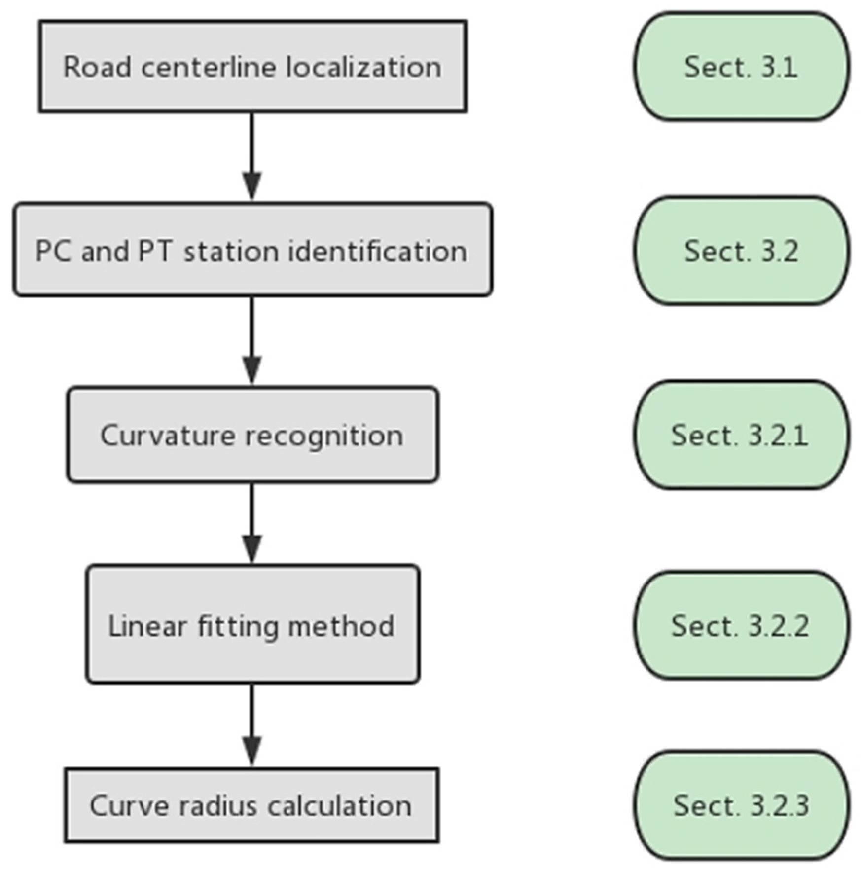
3. Methodology

The research methodology proposed in this study is divided into multiple stages. Firstly, a road centerline location is defined from aerial images based on the actual design of road horizontal alignment. In this method, a set of pixel coordinate points are marked manually midway between the two edges of the single lane of highway ramps; the selected points are then fitted with the best curve that passes through those points to generate a smooth curve that meets the horizontal curve conditions. Secondly, after determining the centerline, a curvature analysis method and linear fitting method are integrated for automatically detecting the PC/PT of curved ramps. After PC and PT are determined, the curve radii are measured automatically using the least-squares fitting method.

3.1. Localization of Road Centerline

The definition of the centerline of the designed road from aerial images is practically challenging. This problem is unusual for rational scientific applications because, in addition to intrinsic errors of the aerial imagery, it is related to the lack of visible markings on the roads that can be followed to determine the centerline, e.g., the centerline of pavement roads, the markings, or others, but these elements are variable over time because of wearing and maintenance works. This paper has developed procedures to define the road centerline based on the actual Chinese standard for road design [30]. The standard states that road trajectory is differently defined according to the roadway cross-section organization: for a single carriageway and one traffic way, the road trajectory is the geometric centerline of the carriageway.

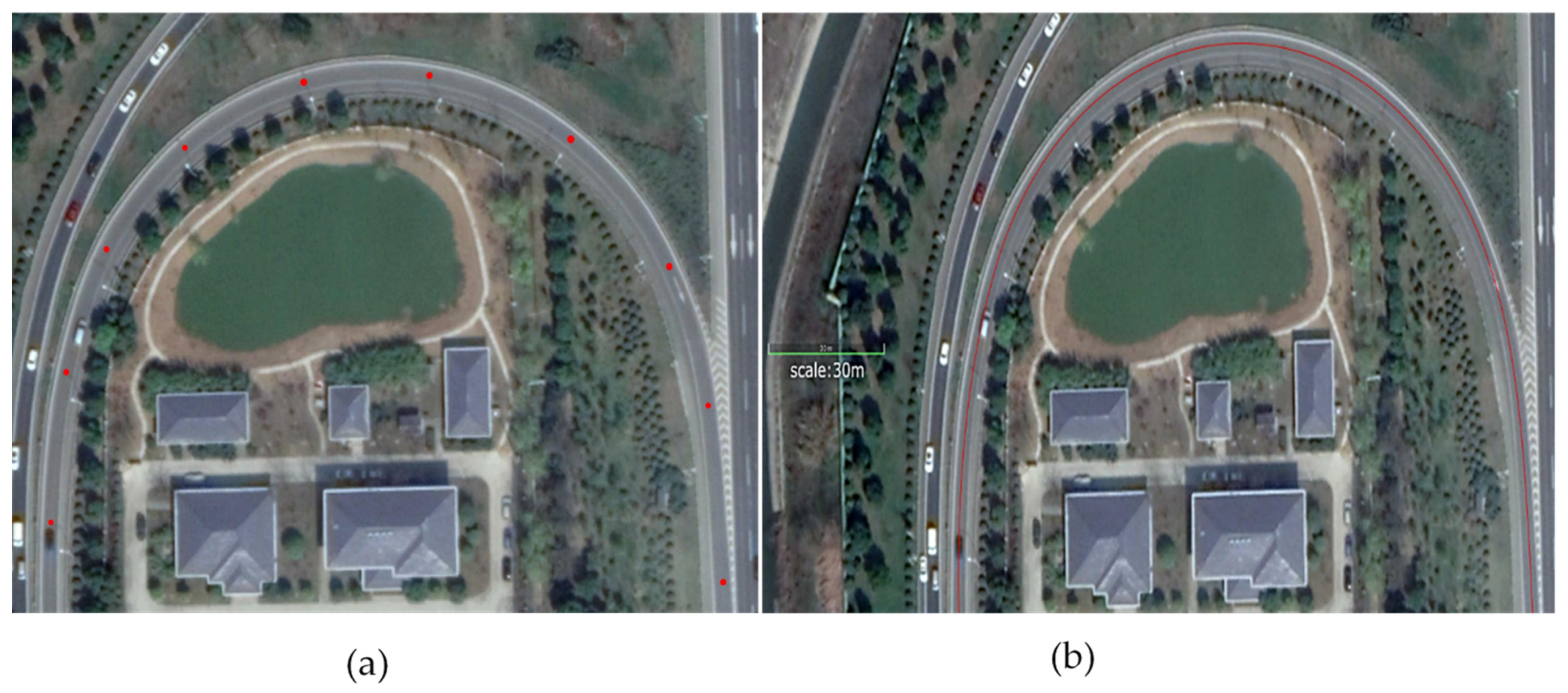
Based on the above procedures, firstly, a set of coordinate points are selected manually along the road lane on the curved ramp, and those points are selected on the middle of a single lane as reference points for the determination of a ramp centerline as shown in Figure 1a. Then, a Bezier curve is used to superimpose the path with the best curve that fits those points, as shown in Figure 1b.

A Bezier curve is a parametric curve that uses Bernstein polynomials as a basic [31]. A Bezier curve of degree $\mathrm{n}$ (order$\mathrm{n}+1$) is represented by:

$$\mathrm{r}\left(\mathrm{t}\right)={{\displaystyle \sum }}_{\mathrm{i}=0}^{\mathrm{n}}{\mathrm{b}}_{\mathrm{i}}{\mathrm{B}}_{\mathrm{i},\mathrm{n}}\left(\mathrm{t}\right), 0\le \mathrm{t}\le 1$$

(1)

The coefficients, bi, are the control points or Bezier points and, together with the basis function Bi,n$\left(\mathrm{t}\right)$, determine the shape of the curved lines drawn between successive control points of the curve from the control polygon.

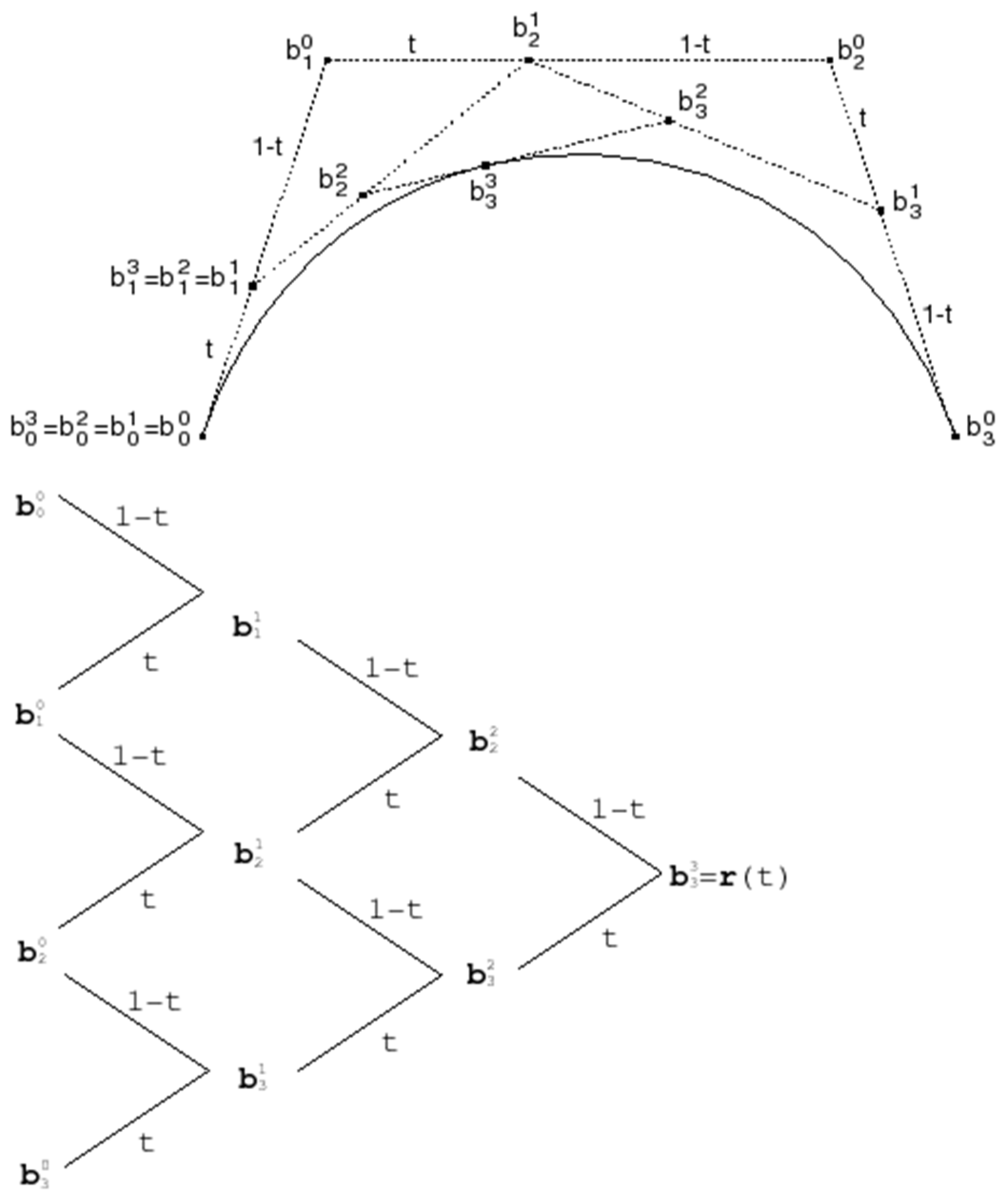
A Bezier curve can be evaluated at a given parameter value t₀, and the curve can be divided at this value using the de Casteljau algorithm Figure 2 [32], recursively applying the following equation to obtain the new control points:

$${\mathrm{b}}_{\mathrm{i}}^{\mathrm{k}}\left({\mathrm{t}}_0\right)=\left(1-{\mathrm{t}}_0\right){\mathrm{b}}_{\mathrm{i}-1}^{\mathrm{k}-1}+{\mathrm{t}}_0{\mathrm{b}}_{\mathrm{i}}^{\mathrm{k}-1},\mathrm{k}=1,2,\dots ,\mathrm{n},\mathrm{i}=\mathrm{k},\dots ,\mathrm{n},$$

(2)

The algorithm is shown in Figure 1 and has the following properties:

• The values ${\mathrm{b}}_{\mathrm{i}}^0$ are the original control points of the curve.
• The value of the curve at parameter value ${\mathrm{t}}_0$ is ${\mathrm{b}}_{\mathrm{n}}^{\mathrm{n}}$.
• The curve is divided at parameter value ${\mathrm{t}}_0$ and can be represented as two curves, with control points (${\mathrm{b}}_{\mathrm{i}}^0,{\mathrm{b}}_1^1,\dots ,{\mathrm{b}}_{\mathrm{n}}^{\mathrm{n}}$) and (${\mathrm{b}}_{\mathrm{n}}^{\mathrm{n}}$,${\mathrm{b}}_{\mathrm{n}}^{\mathrm{n}-1}$,…,${\mathrm{b}}_{\mathrm{n}}^0$).

The method is implemented using the graphics editor Inkscape 1.1. After that, the centerline image file is saved with the scale and imported to Python for the PC/PT detection and curve radius calculation.

3.2. PC and PT Station Identification

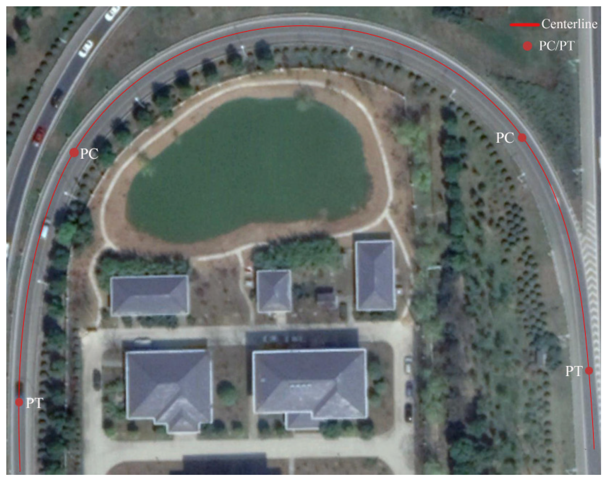
The first step in obtaining the geometric parameters for the horizontal alignment of road curves (i.e., curve radius and curve length) is to correctly identify the PC/PT locations. The curve radii cannot be measured directly if the PC and PT points are not identified. The PC and PT are the connection point between the curved segment and the tangent segment, or two curved segments. Figure 3 illustrates the PC/PT location on a curved ramp. To automatically detect the PC and PT points, the curvature analysis method and the linear fitting methods are integrated to automatically determine the PC and PT points.

3.2.1. Curvature Recognition

On horizontal curves, calculating the curvature value denotes the rotation rate of the tangent direction angle of a certain point to the arc length, indicates the degree of deviation of the curve from the tangent line of the point, or mathematically indicates the degree of curvature of the curve at a certain point [33].

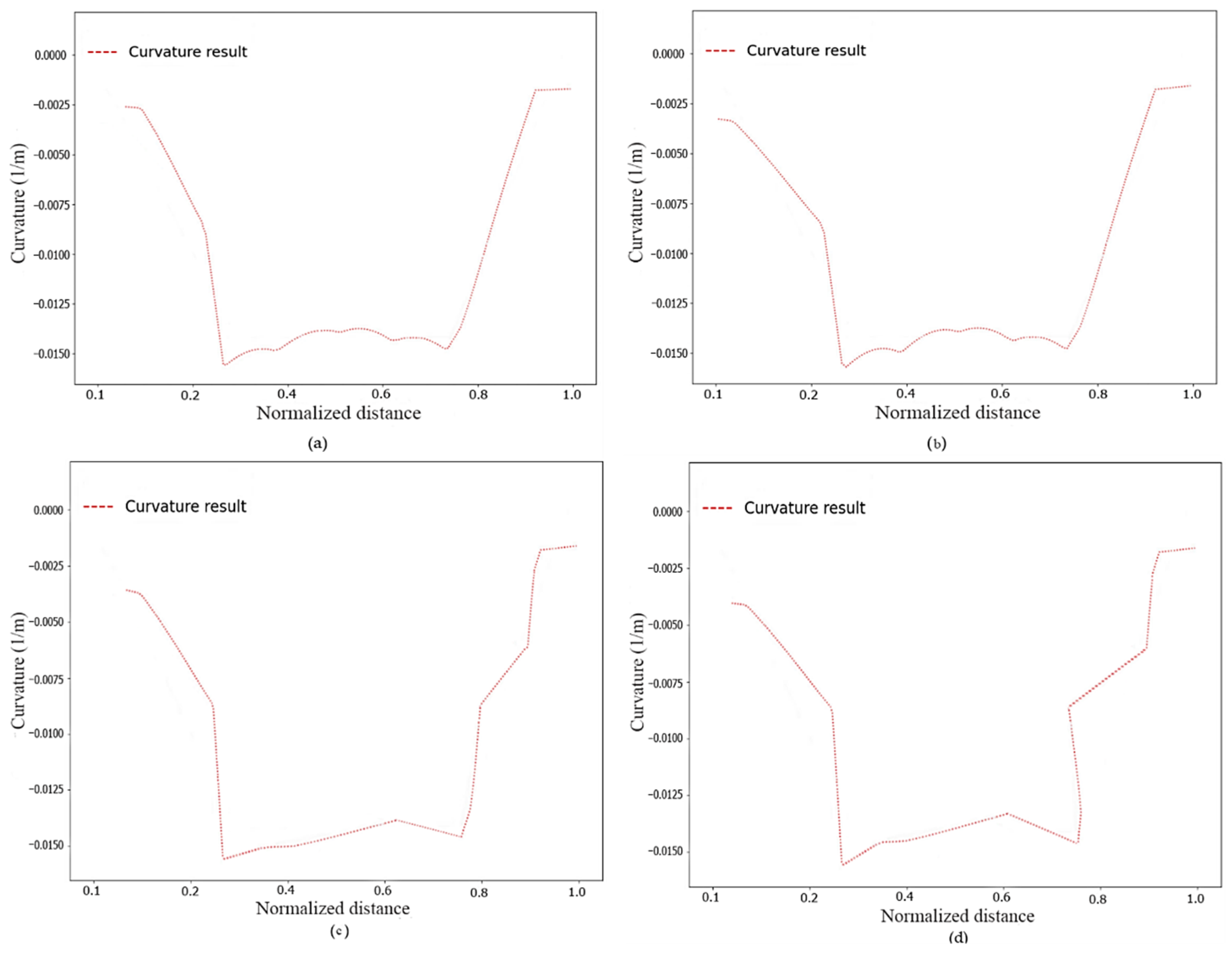
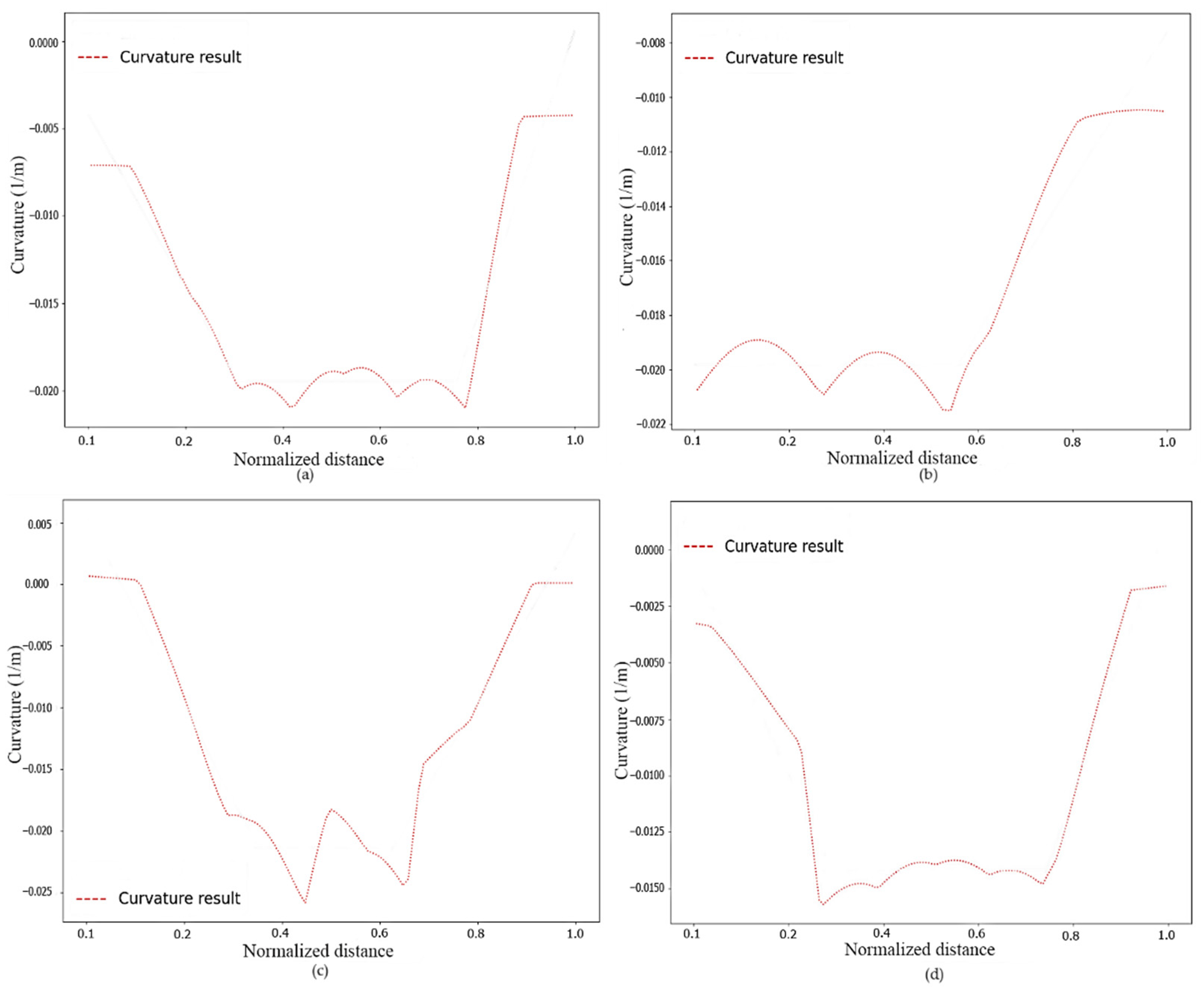
In this study, many curvature computations have been carried out to calculate the curvature at different lengths along the road trajectory using Python. After many attempts, we found that placing the curvature at 2 m positions (Figure 4b) gives a better result; as shown in Figure 4c,d, the greater the distance the greater the decline rate, and vice versa, the smaller the distance the lower the decline rate (Figure 4a) and the greater the number of points, which in turn increases the computational burdens.

The curvature performs as follows:

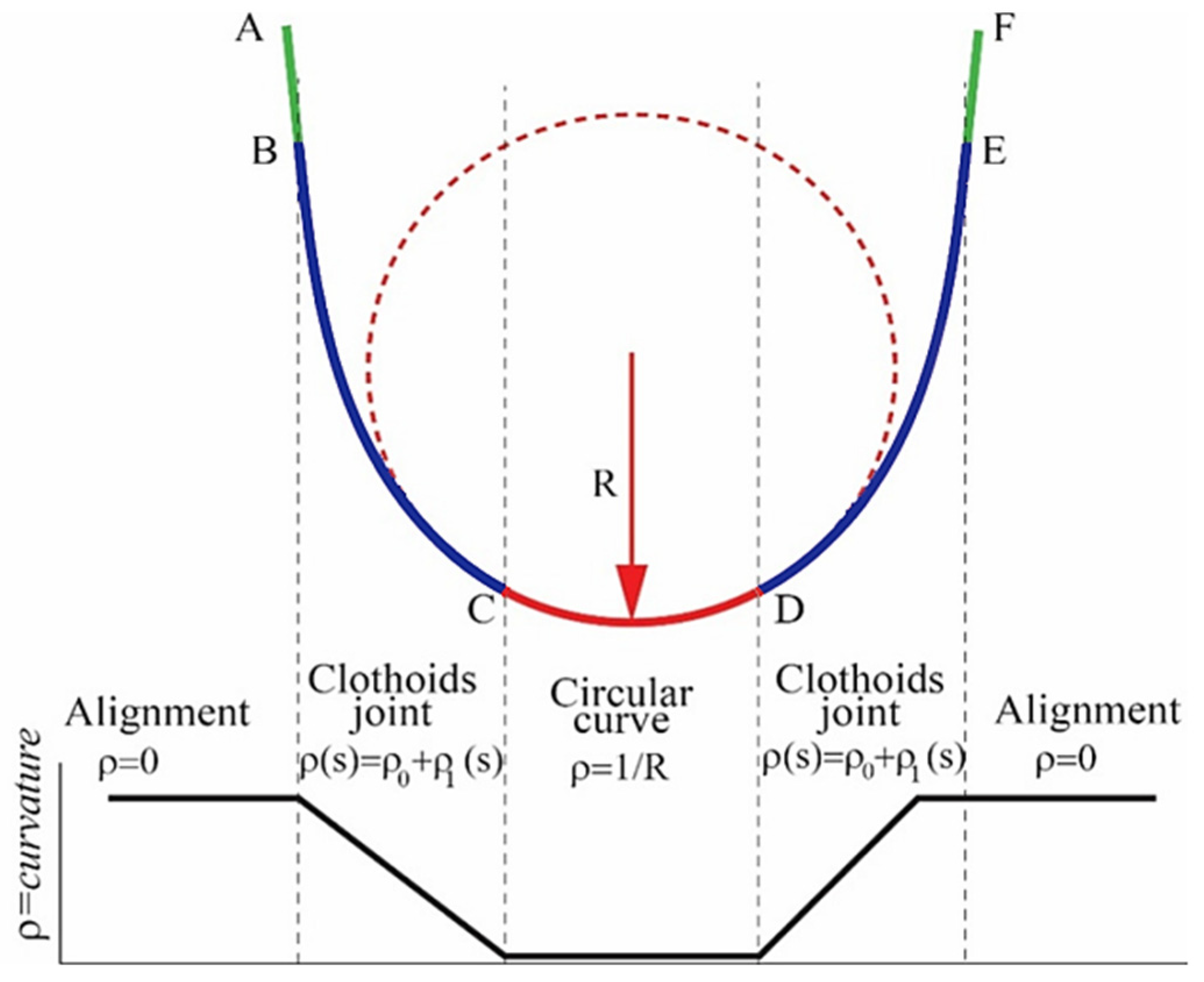
1. The curvature for the straight segments is always equal to zero; 2. The curvature for the circle is a constant value equal to 1/R (curve segment with a fixed radius) Equation (1); 3. The curvature of the transition curve defines the geometry of the Euler spiral [34], the curvature is calculated linearly, and it has a constant rate of change. Figure 5 shows the ideal curvature of a road curve segment by combining two alignments, composed by two clothoids and a circular arc.

$$\mathsf{\rho }=\frac{\mathrm{y}″}{\sqrt[2]{{\left(1+{\mathrm{y}\prime }^2\right)}^3}}=\frac{1}{\mathrm{R}}$$

(3)

• $\mathsf{\rho }$: Curvature;
• ${\mathrm{y}\prime }^2$: First derivative;
• $\mathrm{y}″$: Second derivative;
• $\mathrm{R}$: Radius of curvature;

3.2.2. Linear Fitting Analyses for PC and PT Detection

The difficulty found in the recognition of the PC and PT of the horizontal spiral curve is due to the design characteristics of these curves; the curvature is extremely sensitive to the input parameters. A slight variation can move the transition point between a circle and a transition curve several centimeters to either side, because near the transition point the circle and the spiral are practically the same; when the transition point moves, that changes the length of the spiral. Hence, it is impossible to determine the PC/PT points by detecting exactly the intersection points of the curvature on the transition section.

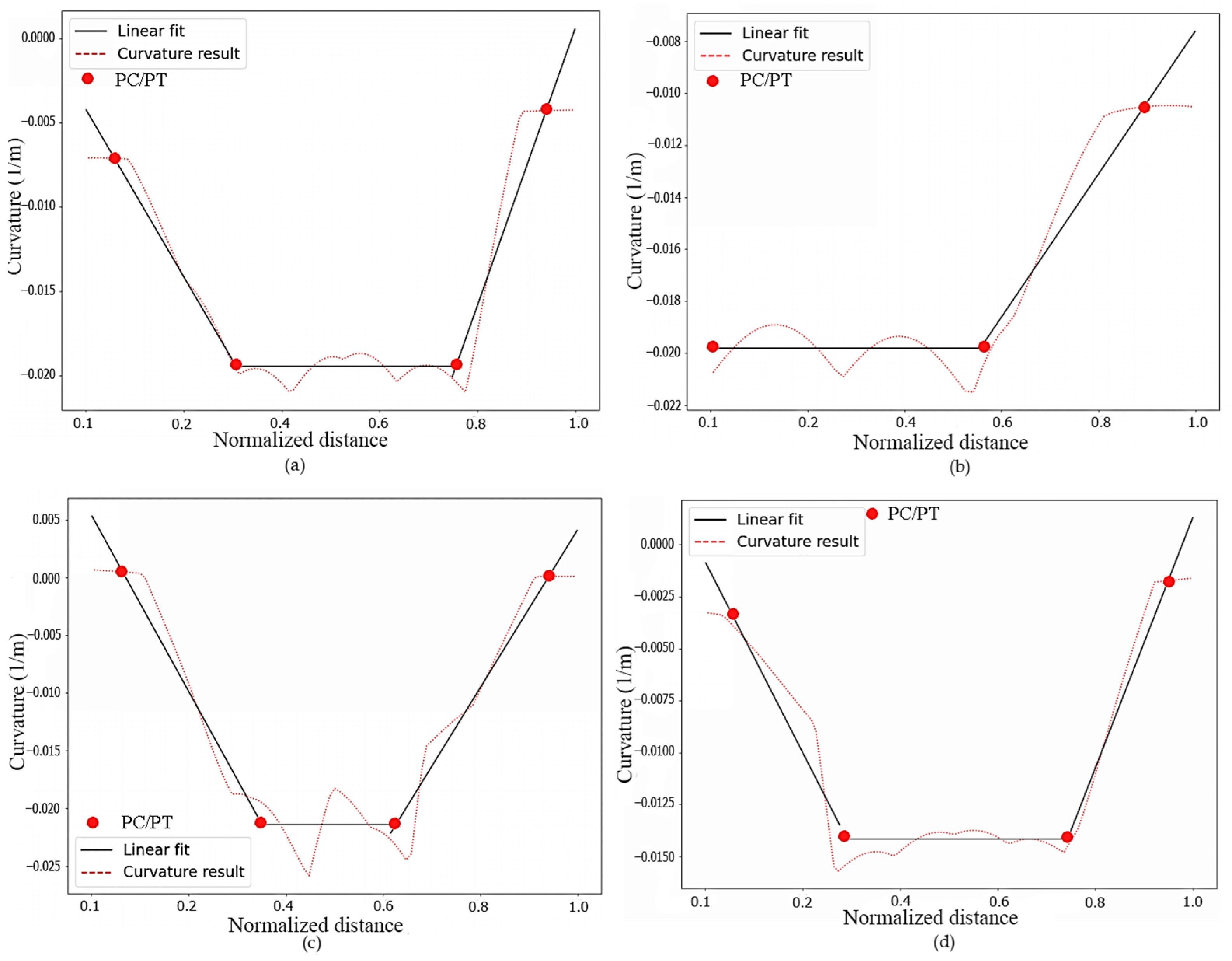
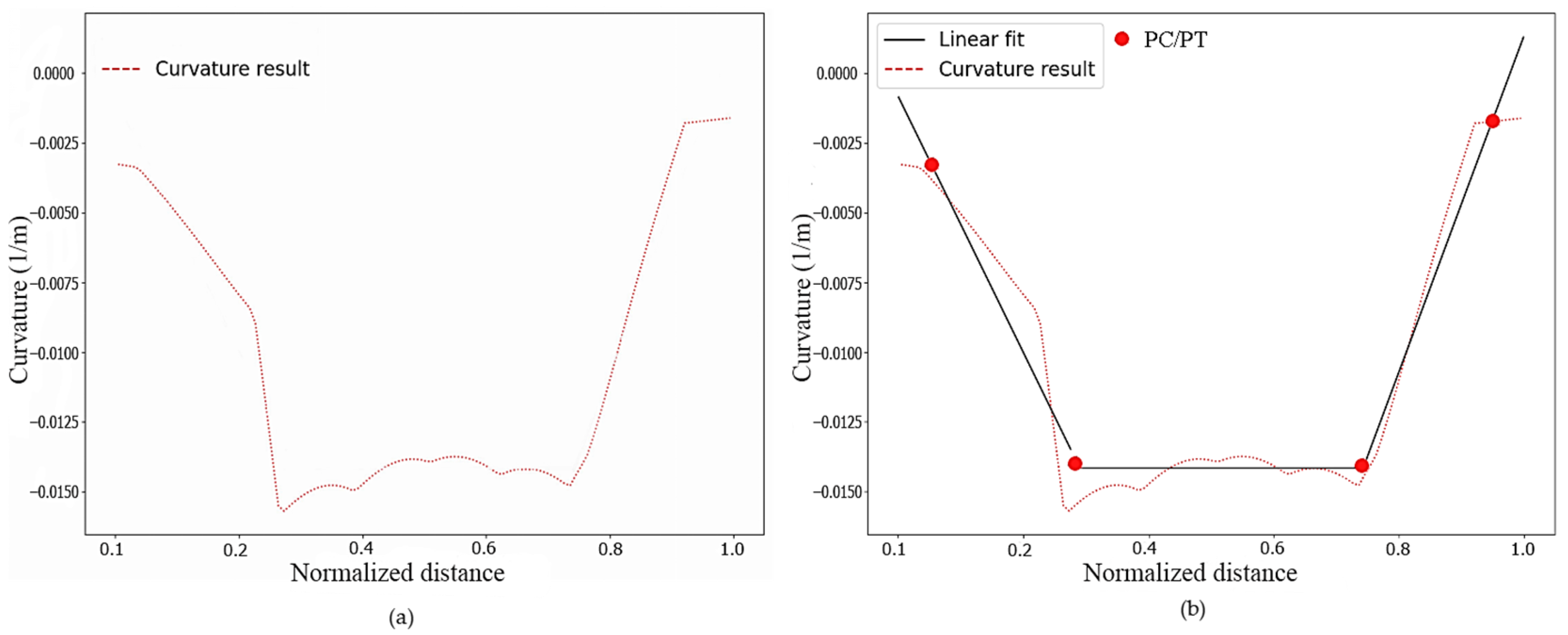
This study proposes a linear fitting-based method to determine the exact positions of the PC and PT of the curved ramps, effectively minimizing the errors caused by the curvature sensitivity to the input data. The data from test site four are taken as an example to show how this method works. Figure 6a shows the curvature profile of the road centerline, and Figure 6b presents the linear fitting result and PT/PT determination calculated from the described procedure. Each segment on the black line corresponds to a piece-wise approximation; horizontal lines indicate arcs or tangents, and inclined parts are spirals. The endpoints of each segment are determined automatically according to the direction of the curvature profile. When the curvature reaches the tangent, it turns into horizontal lines that indicate the endpoints of the curve segment. The x-axis represented the normalized distance along the curved ramp, and the y-axis represented the curvature values. The reason for normalization is to make variables comparable to each other.

3.3. Curve Radius Calculation

After the road centerline is determined and the PC and PT are detected, the identified PC/PT are then marked on the centerline by their x,y coordinates. In this section, the least-squares method is used for curve radius calculation; a Python program was written to perform the various tasks of the presented method. The objective function minimizes the squared deviations between the selected curves and generated curves. After that, an optimization method is used to fit the curved ramp to the data points, using the LS method [35]. Finally, at the post-processing stage, the radii of the curves are computed using basic horizontal curve equations. The proposed method can be applied for simple, compound, and spiral curves.

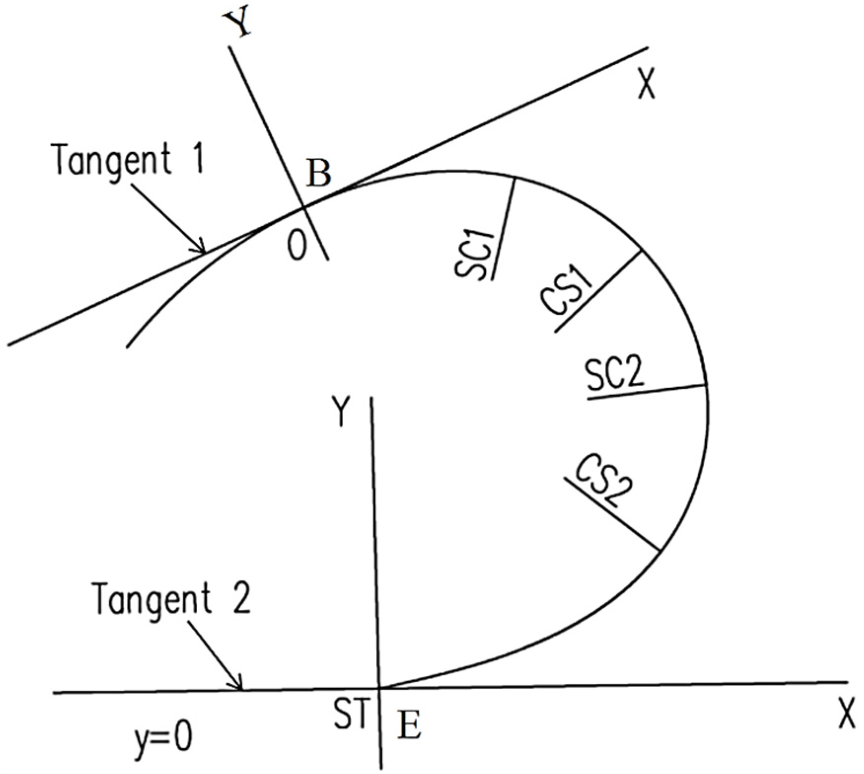
Consider the horizontal curve alignment shown in Figure 7, which consists of a spiral curve at the beginning of the ramp, a circular curve, a spiral, and circular curve in the middle, and an exit spiral, a tangent, at the end. In this figure, B and E represent the starting and ending points. SC represents the transition curve to a circular curve, CS represents the circular curve to the transition curve, and ST indicates the transition curve to the tangent point.

In order to generate and plot the desired curves, including the tangents, the first stage is to code a function that generates and plots the desired roadway curve using all parameters as input. To test the function, the above curve parameters are considered as a sample; seven parameters are considered. “xB” and “yB” are the coordinates of “B”, and they are constant. Parameter “LE” is the length of the straight line at the exit.

After these stages, an objective function is coded, and an optimization function is used to find the parameters minimizing that objective function, which is a norm of the errors. The objective function of the optimization model is written as:

$$\min \mathrm{h}\left({\mathrm{xB},\mathrm{yB}}_{}{,\mathrm{LsE},\mathrm{R}}_2{,\mathrm{tc}2}_{\mathrm{i}}{,\mathrm{LsM},\mathrm{R}}_1{,\mathrm{tc}1}_{\mathrm{i}},\mathrm{Ls}1,\mathrm{LE},\mathrm{xE},\mathrm{yE}\right)=\min {\displaystyle \sum }_{\mathrm{j}=1}^{\mathrm{J}}\Vert {\mathrm{Q}}_{\mathrm{j}}{-\mathrm{W}}_{\mathrm{j}}\Vert {}^2$$

(4)

where h = the objective function, m2, xB1, yB1 = the coordinates of start point “B”, LsE = the length of the spiral curve, R2 = the radius of the circular curve, tc2 = the arc of the circular curve, LsM = the length of spiral curve, R1= the radius of circular curve, and tc1 = the arc of the circular curve. LsI = the length of the spiral curve, LE = the length of straight line at the exit, and xB1 and yB1 = the coordinates of end point “E”. Qj = the selected point in the OXY coordinate, j = the total number of the selected points, Wj = the orthogonal projection of Qj on the alignment, and |Qj − Wj| = the 2- norm or Euclidean norm, representing the residual (difference) between Qj and Wj.

The constraints on the radius and length of the transition curve are given by:

Rmin,i ≤ Ri ≤ Rmax,I,   i = 1, 2,…,I

(5)

Lmin,i ≤ Li ≤ Lmax,I,   i = 1, 2,…,I

(6)

where Rmin, i, Rmax, i = the lower and upper bounds on Ri (m), and Lmin, i, Lmax, i = the lower and upper bounds on Li (m).

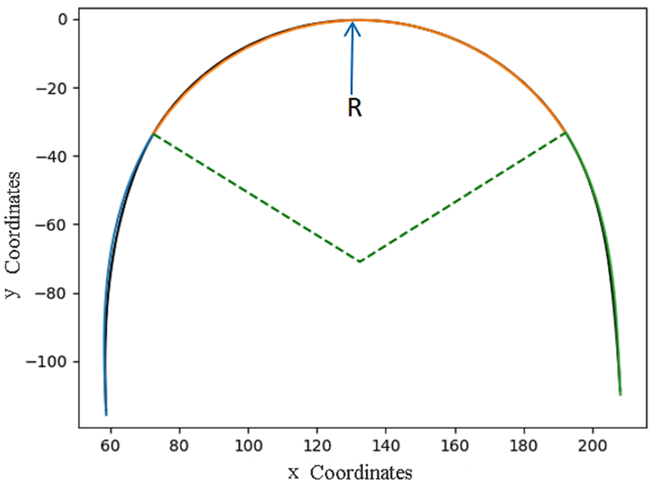
In order to run the code, the start and end positions of each curve segment of the roadway ramp need to be provided. Those positions have been determined based on the PC/PT detected in Section 3.2; then, it will automatically fit the curve on the data with the LS error criterion. The results are presented as shown in Figure 8. The data from test site four are taken as an example to show how this method works.

The spiral parameter (A) is computed using the following formula for each spiral curve:

$$\mathrm{A}=\sqrt{\mathrm{R}\times \mathrm{L}}$$

(7)

where A = the parameter of the spiral, R = radius of the circular cure, and L = length of a spiral.

Figure 9 illustrates the whole data processing procedure for the extraction of the geometric elements of curved ramps.

4. Case Study

Test Sites

In this study, four highway ramps were selected as test sites. The test sites are located in Nanjing, Jiangsu Province, China, as shown in satellite images in Figure 10. The information such as the location of the highways, the number, segment length, and number of the lanes of the ramps at the test sites are shown in

Table 1. The location details of four test sites.

Test Site	Highway	Length (m)	Location		Lanes
			Easting	Northing
1	S 55	287.75	675,744.00	3,518,284.00	1
2	S 88	282.51	679,060.00	3,514,339.00	1
3	S 55	203.05	669,327.00	3,533,951.00	1
4	S 88	298.91	671,488.00	3,524,935.00	1

. The images used in these applications are GE images with a spatial resolution of 2–4 cm/pixel; the images are scaled with the scaling benchmarks provided in each image to return their dimensions to the actual values.

5. Results

5.1. PC and PT Determination

Firstly, curvatures at the test sites were extracted and plotted as shown in Figure 11; the curvature was automatically calculated using Python. Afterward, the linear fitting method was applied to each segment of the curvature data at the four test sites, and results are shown in Figure 12. The PC/PT of the curved ramps was obtained by detecting the intersection points of the fitted straight lines.

5.2. Curve Radius

Figure 13 shows the curvature fitted results between actual and estimated curves at the four test sites. As mentioned in Section 3.3, this study uses the optimization method based on LS to fit the curves to the input parameters, which finds the least of the sum of the square deviations. The curve radius is computed using the horizontal curve Equations (5)–(7).

Table 2. Comparison between extracted data and actual data of horizontal curve.

Test Site	Curve Type	Curve Radius
		Estimated (m)	Reference (m)	Errors (%)
Test site 1	Spiral	75.43	79.77	5.44
	Spiral	58.61	64.61	9.28
	Simple	51.44	50.00	2.88
Test site 2	Spiral	50.94	55	7.38
	Simple	50.47	50.00	0.94
Test site 3	Spiral	59.00	57.50	2.60
	Spiral	62.40	59.00	5.76
	Simple	46.81	45.00	4.02
Test site 4	Spiral	81.87	75	9.16
	Spiral	71.36	75	4.85
	Simple	70.68	70	0.97

shows the results of the proposed method, listing the information about curve radii for each of the test sites (eleven curves in total). The design plans generated in AutoCAD Civil 3D are considered as a reference. The deviation error can be mathematically calculated using Equation (8):

$${\mathrm{E}}_{\mathrm{R}}=\frac{{\mathrm{R}}_{\mathrm{M}}-{\mathrm{R}}_{\mathrm{R}}}{{\mathrm{R}}_{\mathrm{R}}}\times 100$$

(8)

where ${\mathrm{E}}_{\mathrm{R}}$ = errors on the curve radius of the proposed method, %; ${\mathrm{R}}_{\mathrm{M}}$ = the curve radius measured by the proposed method, m; ${\mathrm{R}}_{\mathrm{R}}$ = the reference curve radius, m. The results show that the proposed method successfully determined all the curves’ radii on the four test sites. The percentage difference between the estimated radii and the reference of the simple curves ranges from 0.94% to 4.02%, while the percentage differences between the estimated and the reference of the spiral curves range from 2.60% to 9.28%. The highest percentage differences found in the spirals (test site one and test site four) are due to the slight deviation between the locations of the critical point (CS, SC) of the approximate spiral and circular curve. When estimating the radius of the curve, a difference in length could be a matter of the code being inaccurate by one or two points when locating the PC/PT of the curved ramps.

6. Discussion

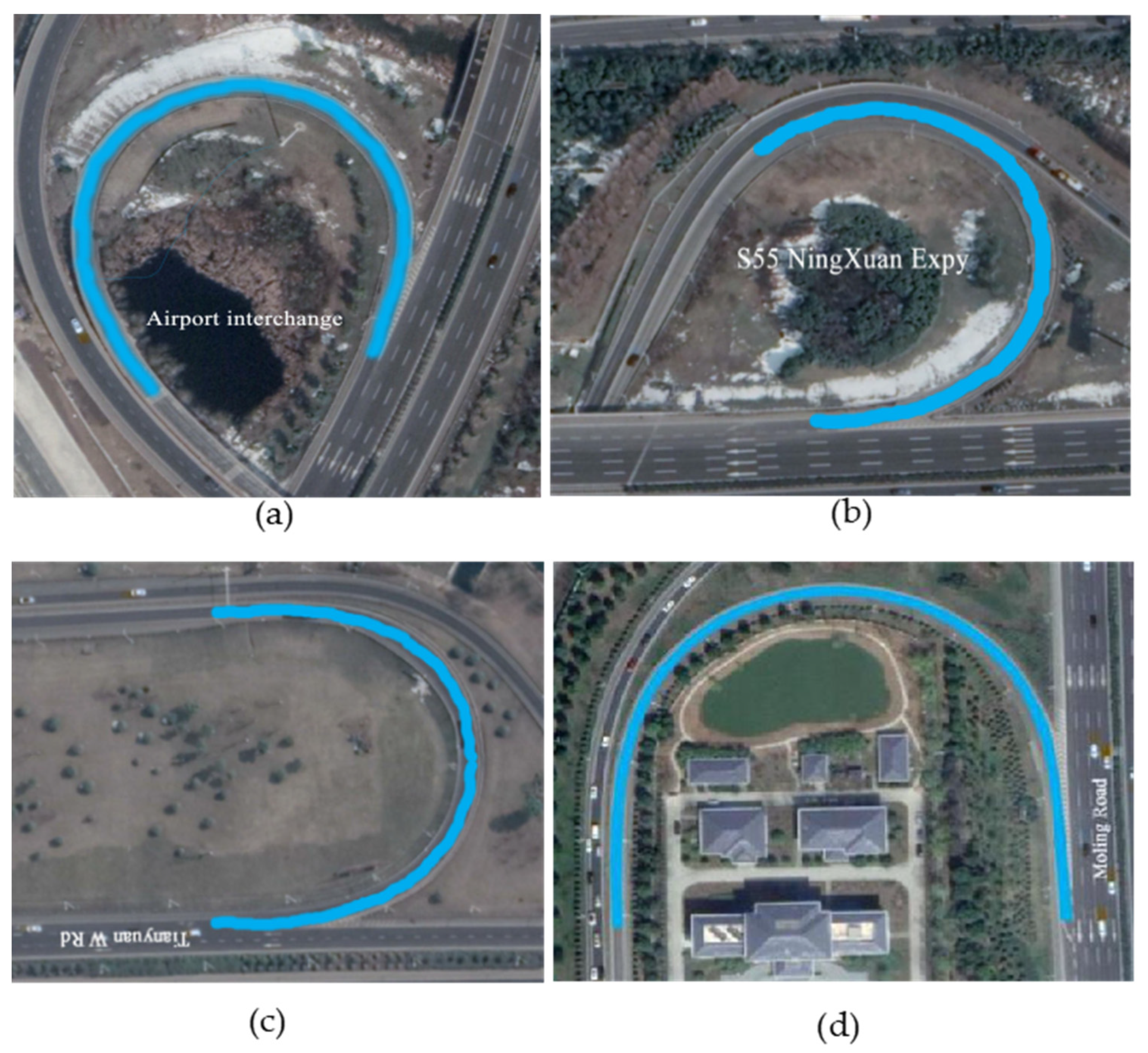
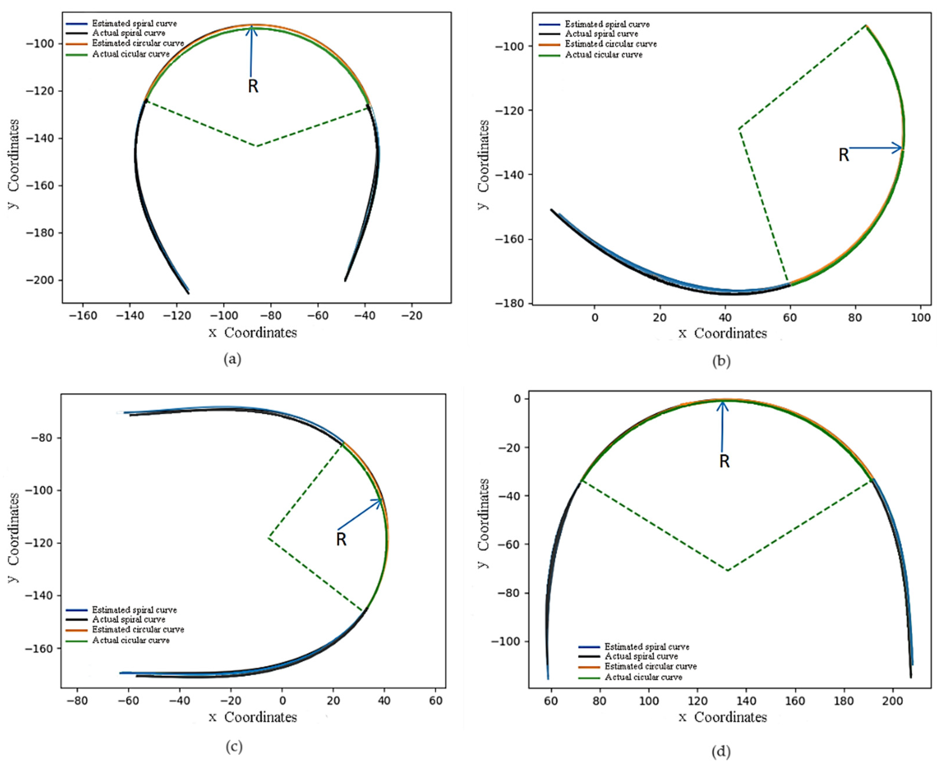
The proposed method was applied to extract four highway ramps that have different characteristics. The highway ramps in Figure 10a,c,d consist of spiral curves connecting a circular and a spiral curve at each end that connect the circular curve and the tangent; the spiral curve has a curvature that gradually begins from 1/R in the entrance to the curvature of the circular curve, Figure 10a. This curve is unsymmetrical, which makes the extraction of the curve more complex. In Figure 10b, the spiral connects one circular curve and the tangent.

The validation results presented in the previous section have demonstrated the effectiveness of the proposed method for extracting horizontal curve information from GE imagery. The results illustrate that the average percentage error for curve radius measurements of the simple curves is 2.20%, which indicates that the proposed method is effective for curve radius measurements. Through validation against actual ground geometric data, the algorithm was also shown to be reliable in extracting the geometric information of curved ramps with high accuracy.

The curvature recognition method and linear fitting method used in this study have proved their effectiveness in determining the highway ramp curve’s PC/PT (Figure 12). However, identification errors were also found during validation. The main reasons for these errors are summarized below:

The typical reason for errors is that the curvature is very sensitive to the input data. The sensitivity analysis showed that the curvature has slight jumps at some points; the reason for this is that the curvature is extremely sensitive to minuscule variations. A slight variation in inputs can move the transition point between a circle and a transition curve several centimeters to either side because the circle and the spiral are practically the same near the transition point. In this case, the spiral segment may have been misidentified as a circular curve by the algorithm, thereby causing this type of error.

7. Conclusions

This paper presents a new method for semi-automatically measuring the horizontal curves of highway ramps, including the PC/PT and curve radii, using Google Earth images. In this study, four test sites located on highway ramps were chosen as testbeds. The conclusions of this study are as follows:

• The data points were first selected along the road trajectory using a graphics editor software and fitted with the best curve that passes through those points to generate a smooth curve that meets the horizontal curve conditions.
• The curvature analysis method was used for automatic PC/PT location search, and the linear fitting analysis method was applied for exact PC/PT localization. After the PC and PT were located, the road curves were measured using the total least-squares fitting method.
• The presented method was validated by comparing the estimated results against a road with known data. The results show that the proposed method successfully identified the spiral transition from circular curves and extracted their curve radii with an average error of 2.20% for simple curves and 6.35% for spiral curves. The proposed method presented a virtual extension to existing methods for obtaining horizontal curve information and should be of interest to surveying professionals. This helps reduce the burden associated with traditional surveying tools. The applications of the developed algorithm range from providing real-time information about curve geometry to drivers and autonomous vehicles to using the extracted data in safety-prediction models to improve safety on curves.
• The precision of GE images may contribute to the errors in the extraction of horizontal curve parameters. Future research focusing on a fully automatic extraction method might reduce the errors and increase the overall identification rate. Drone images may also be used to enhance the accuracy of obtaining the geometric information of horizontal curves.