Article

A Metaheuristic-Based Micro-Grid Sizing Model with Integrated Arbitrage-Aware Multi-Day Battery Dispatching

1
Sustainable Energy Systems, Wellington Faculty of Engineering, Victoria University of Wellington, Wellington 6140, New Zealand
2
Department of Industrial Engineering, Stellenbosch University, Stellenbosch 7600, South Africa
*
Author to whom correspondence should be addressed.
Sustainability 2022, 14(19), 12941; https://doi.org/10.3390/su141912941
Submission received: 6 September 2022 / Revised: 3 October 2022 / Accepted: 7 October 2022 / Published: 10 October 2022
(This article belongs to the Special Issue The Role of Storage and Demand Response in Sustainable Energy Systems)

Abstract

:
Rule-based micro-grid dispatch strategies have received significant attention over the last two decades. However, a recent body of literature has conclusively shown the benefits of operational scheduling optimisation while optimally sizing micro-grids. This is commonly referred to as micro-grid design and dispatch co-optimisation (MGDCO). However, as far as can be ascertained, all the existing MGDCO models in the literature consider a 24-h-resolved day-ahead timeframe for the associated optimal energy scheduling processes. That is, intelligent, look-ahead energy dispatch strategies over multi-day timeframes are generally absent from the wider relevant literature. In response, this paper introduces a novel MGDCO modelling framework that integrates an arbitrage-aware linear programming-based multi-day energy dispatch strategy into the standard metaheuristic-based micro-grid investment planning processes. Importantly, the model effectively extends the mainstream energy scheduling optimisation timeframe in the micro-grid investment planning problems by producing optimal dispatch solutions that are aware of scenarios over three days. Based on the numeric simulation results obtained from a test-case micro-grid, the effectiveness of the proposed optimisation-based dispatch strategy in the micro-grid sizing processes is verified, while retaining the computational tractability. Specifically, comparing the proposed investment planning framework, which uses the formulated 72-h dispatch strategies, with the business-as-usual MGDCO methods has demonstrated that it can reduce the micro-grid’s whole-life cost by up to 8%. Much of the outperformance of the proposed method can be attributed to the effective use of the behind-the-meter Li-ion battery storage, which improves the overall system flexibility.

1. Introduction

1.1. Background and Motivation

Micro-grids (MGs) are typically associated with high capital and replacement costs, but low operation and maintenance costs [1,2]. This makes the global (true) optimisation of the MG resources especially important, especially in efforts to accelerate the transition to renewables. In particular, the system integration of a high share of non-dispatchable and weather-dependent renewable energy sources (RESs), such as solar photovoltaic (PV) panels and wind turbines (WTs), into MGs adds significant computational complexities to the conventional micropower system design problem. In addition to dealing with the high capital costs of RESs and the variability in their power outputs, there is a wide variety of operational- and planning-level constraints that need to be simultaneously met while optimally designing an MG [3,4,5].
Further compounding the MG design problem is the consideration of stationary batteries as they increase the dimensionality of the problem at hand. Accordingly, the optimal charge/discharge coordination of batteries can have a significant impact on the cost-effectiveness of MG solutions. This is particularly salient in off-grid MG installations where there exists no connection to the wider utility grid to help in serving the peak load and/or absorbing the excess generation. Accordingly, there is a great risk of sub-optimality in MG designing problems, with potential overbuilt capacity or inadequate reliability implications [6,7].
In this light, integrating an economic multi-day, forward-looking energy dispatch optimisation framework into the design processes of MGs is widely found to be able to provide new layers of insight and perspective into the MG investment planning problem. More specifically, the objective of the MG design and dispatch co-optimisation problem is to balance the cost of capital investment with the expected total operational cost, subject to a set of technical feasibility constraints. Estimating the associated total operational costs generally entails simulating the energy scheduling and capacity procurement using forecasts of input data—electricity demand, local renewable generation, and wholesale prices—for a typical year at a given resolution [8,9].

1.2. Literature Review

A recent growing body of literature has recognised the importance of optimising the energy dispatch over a forward-looking time horizon, while optimally planning renewable and sustainable energy systems [10,11]. For instance, Li et al. [12] proposed an evolutionary computation-based MG sizing model with integrated mixed-integer linear programming (MILP)-based unit commitment decisions. In another instance, Swaminathan et al. [13] developed a genetic algorithm-based MG sizing modelling framework with a nested model predictive control-oriented daily energy management strategy tailored to the battery energy storage systems (BESSs) of commercial buildings. Similarly, Xiao et al. [14] formulated a bi-level metaheuristic-based MG capacity planning model where the economic dispatch problem is solved in the inner loop using an improved variant of the particle swarm optimisation algorithm, whereas the optimal designing problem is solved in the outer loop using the mesh adaptive direct search algorithm. Furthermore, Chen et al. [15] have put forward a two-stage robust optimisation model to co-optimise the operational scheduling and investment planning costs of an energy hub considering an ellipsoidal uncertainty set to address the variability inherent in input data. Moreover, Subramanyam et al. [16] proposed an integrated optimal MG planning model to simultaneously allocate distributed energy resources and determine the daily operating schedules. Table 1 provides an overview of the notable existing work on the design and dispatch co-optimisation of MG, whilst also positioning the novelties of this study within the identified gaps in knowledge.

1.3. Knowledge Gaps

Although a growing body of research has supported the role of operational planning optimisation during the long-term investment planning phase in minimising the so-called simulation-to-reality gaps, the significance of optimising the energy scheduling over multiple operating days, rather than a 24-h horizon, is less explored. In response, this paper seeks fundamentally to address this knowledge gap by presenting a joint optimisation framework for investment planning and operational scheduling of the distributed energy infrastructure integrated into grid-connected, battery-supported, renewables-driven MGs, which is necessary for improving the dispatchability of 100%-renewable MGs using more intelligent energy dispatch decisions that consider wider timeframes.
In addition, Table 1 is revealing as to the less scholarly attention given to the consideration of arbitrage-aware optimal dispatch strategies (in an integrated way) in the associated stochastic methods focusing on the optimal system configuration and unit sizing of renewable and sustainable energy systems. More specifically, whereas all the identified relevant scholarly publications promote an integrated design and dispatch optimisation model, the potentially significant benefits of using the onsite storage for arbitrage operations have been widely overlooked. That is, the table demonstrates that no single article, as far as can be ascertained, has effectively valued the arbitrage economics of energy storage during the long-term strategic investment planning phases of renewable and sustainable energy systems.

1.4. Novel Contributions

In response to the identified knowledge gaps, this paper first introduces a novel forward-looking 72-h energy storage scheduling optimisation framework based on linear programming. The proposed energy dispatch framework is subsequently nested within a standard metaheuristic-based MG capacity planning optimisation model for associated impact analyses. More specifically, the major contributions of this study are as follows:
  • Formulating a robust metaheuristic-based MG equipment capacity planning optimisation model tailored towards community-scale, 100%-renewable and -reliable energy projects.
  • Developing an arbitrage-aware, dynamic, look-ahead, predictive dispatch strategy for the optimal scheduling of MGs—charging/discharging of energy storage systems and energy exchanges with the main power grid—over a moving 72-h dispatch horizon.
  • Nesting the developed forward-looking operational planning problem—formulated to optimally respond to the dynamic nature of system conditions over a moving three-day period—within the proposed metaheuristic-based MG sizing model to jointly optimise the design and dispatch of MG systems.
Importantly, for the first time in the literature, this study has shown how integrating computationally tractable optimisation-based dispatch strategies over multi-day horizons, rather than business-as-usual rule-based strategies and state-of-the-art daily strategies, into metaheuristic-based MG sizing modelling frameworks can minimise the risks of overbuilt RESs. The outperformance of the proposed integrated design and dispatch co-optimisation model to the existing frameworks in the relevant literature has been validated using a comprehensive two-way sensitivity analysis, which additionally verifies the statistical robustness of the model.

1.5. Paper Organisation

The remainder of this paper is organised as follows. Section 2 mathematically formulates a test-case MG. Section 3 presents the method parametrised for the test-case system of interest. Section 4 presents and discusses the numerical simulation results for a case study by populating the model with real-world data. Finally, conclusions are drawn and prospects for future work are outlined in Section 5.

2. Test-Case Micro-Grid
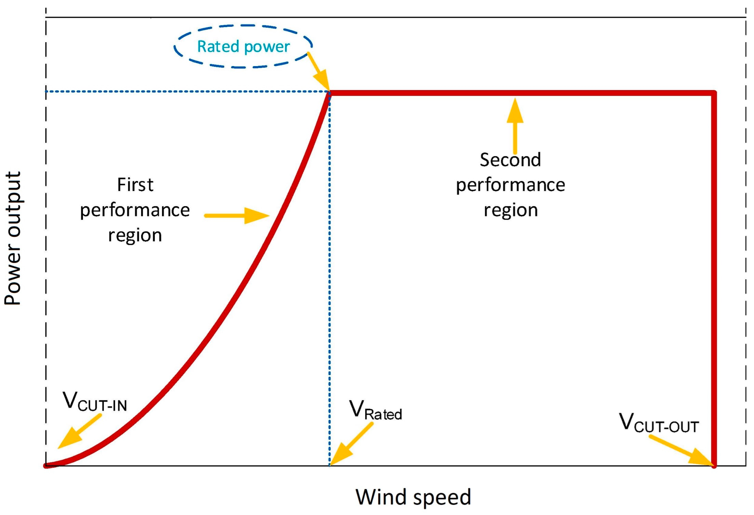
In accordance with Figure 1, a grid-tied, DC-coupled community-scale MG is formulated to test the effectiveness of the proposed integrated MG sizing and scheduling framework. As the figure shows, the conceptual MG integrates solar photovoltaic (PV) panels, wind turbines (WTs), a stationary Li-ion (lithium iron phosphate) battery bank cycled at a C/2 rate, and a multi-mode inverter. A detailed mathematical formulation of the MG components is presented in the following sub-sections. It is noteworthy that the transformer and the multi-mode inverter are independently modelled by their efficiencies. However, the efficiencies of the converters connecting the solar PV panels, WTs, and the battery bank to the common DC busbar are factored in the mathematical models of the corresponding component. Furthermore, a fixed power factor of 95% was assumed. However, the model is generally applicable to other power factors as well, as this parameter is principally used to constrain the power exchanges with the wider utility network, in accordance with the size of the transformer as the point of common coupling.
The following sub-sections provide the mathematical formulation of the components of the MG.

2.1. Wind Turbines

To determine the power output of the WT generator, the wind speed data (m/s), measured at the height of h r e f (m), needs to be converted to the hub height h using the power law equation, as follows [26]:
V h = V r e f   × ( h / h r e f ) r ,
where V r e f is the wind speed (m/s) at the anemometer height h r e f (m) and r is the power law exponent, which is fixed at 0.2 in this study given the flat, lightly tree-covered terrain characteristics of the site of interest [27].
The power output from each WT can then be determined as follows [26]:
P W T ( t ) = { 0 i f   v ( t ) < v c i n   o r   v ( t ) > v c o u t P r a t e d × ( v ( t ) 3   v c i n 3 v r a t e d 3   v c i n 3 ) i f   v c i n v ( t ) < v r a t e d P r a t e d i f   v r a t e d v ( t ) < v c o u t
where P W T ( t ) is the WT’s output power (kW) at time-step t , P r a t e d is the rated power (kW), whereas v ( t ) ,   v c i n , and v c o u t , respectively, denote the nominal wind speed, cut-in wind speed, and cut-out wind speed (m/s) of the WT. Figure 2 characterises the power curve of a representative WT [28].

2.2. PV Panels

The following equations express the power output from each PV panel (kW) at time-step   t [29]:
P P V ( t ) = D F × G T ( t ) × A S × η P V ( t ) / 1000 ,
η P V ( t ) = η r η p c [ 1 μ ( T c ( t ) T c , r e f ) ] ,
T c ( t ) = T a ( t ) + [ N O C T T a ,   N O C T G T , N O C T ] G T ( t ) ,  
where G T ( t )   is the global solar irradiance (W/m2) at time-step t , D F is the degradation rate, A S is the panel’s surface area (m2), η r denotes the panel’s efficiency, η p c is the built-in inverter’s efficiency, μ denotes the PV temperature coefficient of power (%/°C), T c , r e f denotes the reference cell temperature (°C), T c ( t ) is the effective cell temperature (°C), N O C T represents the nominal operating cell temperature (°C), whereas T a , N O C T and G T , N O C T , respectively, denote the ambient temperature (°C) and solar irradiance (W/m2) at nominal operating cell conditions.

2.3. Battery Storage

The following equation is used to determine the battery bank’s state of charge (SOC) at each time-step t [30]:
E B ( t ) = E B ( t 1 ) × ( 1 σ ) +   P c h ( t ) × η c h P d c h ( t ) / η d c h N B × E B , r × Δ t ,
where P c h   and   P d c h , respectively, denote the charging power and discharging power of the battery bank (kW), N B denotes the optimal quantity of battery packs integrated into the battery bank, σ is the self-discharging rate (fixed at 0.3% per day in this paper [31]), E B , r denotes the rated energy capacity of each battery pack (kWh), whereas η c h   and η d c h , respectively, denote the charging and discharging efficiencies of the battery storage, which are fixed at 95% in this paper [32].
Additionally, the charging power and discharging power of the battery storage at each time-step can be determined as follows [2]:
  P c h ( t ) = min ( N B × P c h m a x ,   E B m a x E B ( t ) η c h Δ t ) ,            
  P d c h ( t ) = min ( N B × P d c h m a x ,   ( E B ( t ) E B m i n ) × η d c h Δ t ) ,        
where P c h m a x is the maximum charging power capacity, P d c h m a x is the maximum discharging power capacity, E B m i n is the minimum allowed energy in-store, and E B m a x is the maximum allowed energy in-store.
Furthermore, the three-point rainflow-cycle-counting algorithm [33] is used to quantify the heterogeneous cycles of the battery bank. Figure 3 illustrates the application of the rainflow-cycle-counting algorithm to a typical battery SOC profile [33]. The yellow triangles in the figure represent the full cycles, whereas the blue triangles represent the half-cycles of the battery bank. Specifically, the representative SOC profile contains three full cycles of B-A′-B′, J-K′-J′, and I-F-I′, as well as four half-cycles of C-D-C′, G-H-G′, L-M-L′, and N-O-N′. In this study, MATLAB’s built-in ‘rainflow’ function is used to estimate the battery cycle counts.

2.4. Inverter

The following equations are used to model the multi-mode inverter of the MG [34]:
η i n v = P o P r P o P r + η o + m ( P o P r ) 2 ,      
η o = 10 η 10 1 η 100 9 99 ,                        
m = 1 η 100 η o 1 ,
where P o denotes the inverter’s power output, P r is the inverter’s rated power, m is a coefficient employed to obtain the best-fit curve of the manufacturer-provided inverter efficiency data, whereas η 10 and η 100 , respectively, denote the efficiency of the inverter at 10% and 100% rated power.

3. Methodology

This section presents the proposed model for the co-optimisation of the design and dispatch of grid-connected MGs in a two-layer structure. To this end, it first briefly explains the temporal arbitrage opportunities that the optimal dispatch problem seeks to exploit. It then proceeds to formalise and mathematically formulate the proposed two-stage modelling framework for the optimal sizing and scheduling of MGs before illustrating the associated interactions of the two sub-problems at hand using a flowchart.

3.1. Targeted Arbitrage Opportunities

In this study, temporal energy arbitrage not only refers to buying energy at a low price, storing it, and selling it later at a higher price, but it also incorporates the strategy of storing the excess onsite generation for later, more remunerative exports (using renewables to charge storage when electricity prices are low and then discharging it when demand and prices are higher), as well as later discharge of the energy stored by lower-priced imports and excess generation to local loads during the coincident peak periods. In this setting, the general arbitrage strategy of ‘buy low, sell high’—which fundamentally seeks to take advantage of future price variations—can additionally be interpreted as ‘buy low, sell reasonably’. In battery energy management terms, this can be expressed as ‘charge cheaply, discharge foresightedly’ to effectively prioritise taking advantage of low market prices for maximum imports over non- to slightly-profitable exports for the model instances with fixed, low to moderate feed-in tariff rates.

3.2. Optimal Capacity Planning Problem

The capacity planning optimisation problem represents the outer-layer problem with the overall objective of minimising the total net present cost (TNPC) of the MG, as [35]:
min T N P C = c C N P C c + N P C ( P i m n e t ) + p f ,  
where N P C c denotes the net present cost of MG component   c C , N P C ( P i m n e t ) denotes the net present cost of the net imported energy over the MG life-cycle, whereas the term p f adds a sufficiently large penalty to infeasible solutions.
Additionally, the net present cost (NPC) for each MG component   c C can be expressed as [36]:
N P C c = N c × ( C C c + R C c × S P P W + C O & M , c C R F ( i , R ) S V c ) ,
where N c denotes the optimal capacity returned at each iteration of the optimisation process, whereas C C c , R C c , and C O & M , c , respectively, denote the capital cost, replacement cost, as well as the operation and maintenance cost of component c . Further, S P P W and C R F , which, respectively, denote the single payment present worth factor and capital recovery factor, are used to determine the future value of a stream of cash flows. Additionally, i and R respectively denote the real interest rate and the expected project lifetime, whereas S V c denotes the salvage value of component c .
Specifically, the single payment present worth factor, S P P W , and the capital recovery factor, C R F , can be expressed as follows [36]:
S P P W = n = 1 Y 1 ( 1 + i ) L × n ,  
C R F ( i , R ) = i ( 1 + i ) R ( 1 + i ) R 1 ,  
where Y = [ R L ] with R denoting the life-cycle of the project in years (in this analysis, 25 years) and L denoting the expected lifetime of the component, the NPC of which is being calculated. Further, i denotes the real interest rate, which is fixed at 4% in this paper.
Moreover, each asset’s salvage value be determined as follows [36]:
S V c = R C c × L ( R L × [ R L ] ) L .  
To ensure that the planning-level objective function adequately adheres to the physical limitations whilst providing long-term strategic objectives, the relevant objective function in Equation (12) must adhere to a set of constraints, including the reliability of power supply, upper limits on the design variables, as well as the initial and terminal energy stored in the battery bank.
More specifically, the equivalent loss factor (ELF) is employed to measure the reliability of each system design (a specific combination of capacities of the components), which can be mathematically expressed as [37]:
E L F L = 1 T t = 1 T Q L ( t ) P L ( t ) ,
where T denotes the total number of time-steps considered for the associated year-long operational analysis, whereas P L ( t ) and Q L ( T ) , respectively, denote the demanded load and lost load at time-step t.
As the following equation expresses, the total lost load is enforced to be equal to 0:
E L F L = 0 .
Additionally, the constraints in Equations (19) and (20) define the initial and terminal energy contents of the battery bank, whereas the constraint in Equation (21) limits the solution space to minimise the risk of computational intractability [38,39,40]. More specifically, Equation (20) represents a terminal battery capacity constraint which ensures that the year-end energy content of the battery bank equals or exceeds its initial capacity (which is set to be full as in Equation (19)), whereas Equation (21) specifies the upper bounds on the non-negative size of the components.
E B ( 0 ) = N B × E B , r   ,  
E B ( T ) E B ( 0 ) ,
0 N c N c m a x ,   c
where E B ( 0 ) is the initial energy content of the battery bank, E B ( T ) is the energy content of the battery bank at the terminal time-step of the year-long operational analysis, and N c m a x denotes the maximum allowable size of component c .

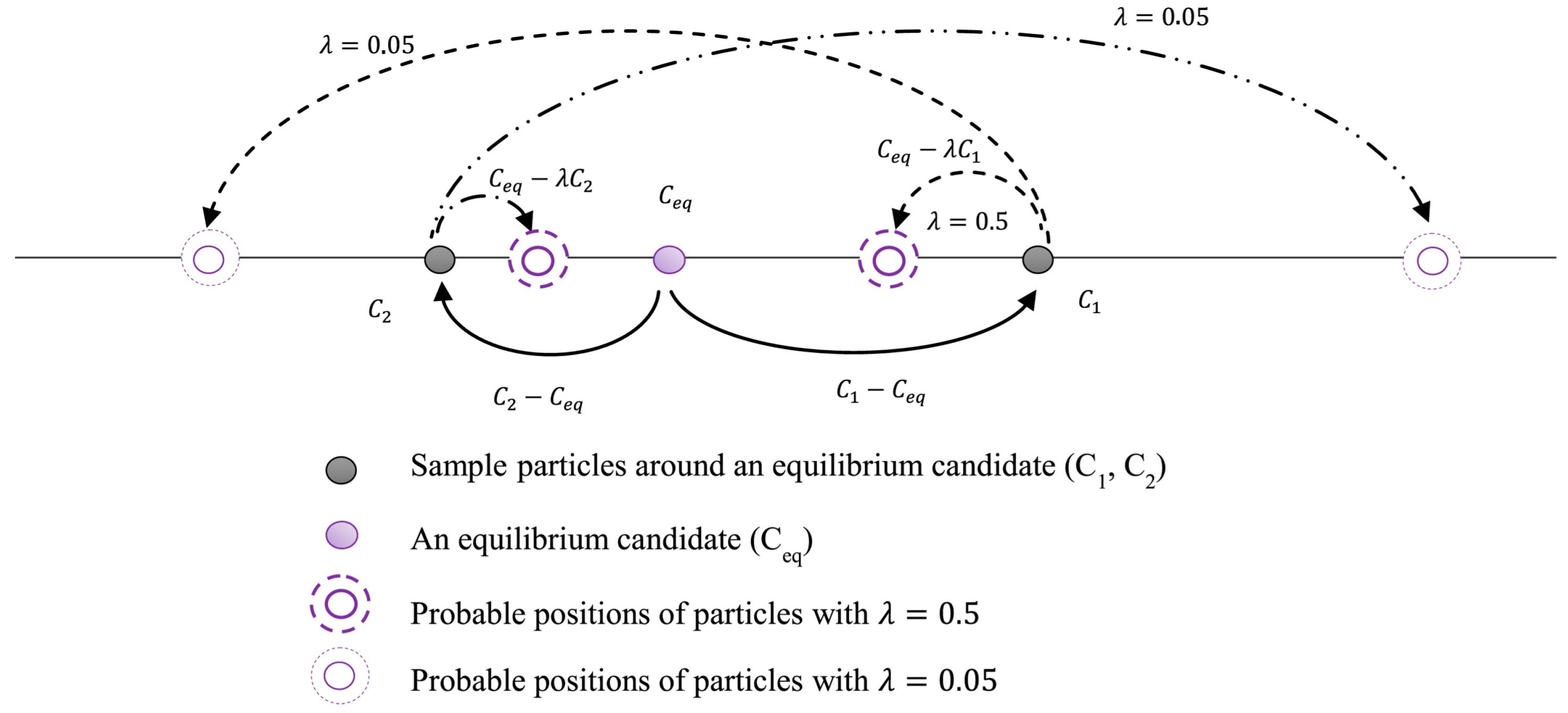
Metaheuristic Optimisation Algorithm

To optimise a solution to the planning-level problem subject to the imposed constraints, a newly developed metaheuristic optimisation algorithm, namely the equilibrium optimiser (EO) [41], is used in this study. The EO was chosen due to its unique advantages in trading off the exploration and exploitation phases of searching the solution space. Such trade-offs are essential for increasing the accuracy of the solution whilst ensuring the computational tractability in the highly-dimensional and computationally-intensive MG sizing problem. Accordingly, the original developers of the algorithm have conclusively shown its statistically significant outperformance to a wide range of metaheuristics in solving high-dimensional, non-convex, nonlinear problems in polynomial time [41].
The EO is inspired by the concept of “a simple well-mixed dynamic mass balance on a control volume, in which a mass balance equation is used to describe the concentration of a nonreactive constituent in a control volume as a function of its various source and sink mechanisms” [41]. The mass-balance equation, which forms the underlying equation of the EO can be expressed as [41]:
V d C d t = Q C e q Q C + G ,    
where C is the concentration inside the control volume denoted by V , whereas V d C d t represents the rate of change of mass in the control volume. In addition, Q is the volumetric flow rate into and out of the control volume, whereas C e q is the concentration at an equilibrium state with no generation inside the control volume. Further, G denotes the mass generation rate inside the control volume.
In this setting, similar to most search agent-based metaheuristics, the EO is initialised as follows [41]:
C i i n i t i a l = C m i n + r a n d i ( C m a x C m i n ) ,                 i = 1 , 2 , , n  
where C i i n i t i a l is the initial concentration vector of the i -th search agent, C m i n and C m a x , respectively, denote the minimum and maximum values of the dimensions, r a n d i is a random number in the range [0, 1], whereas n denotes the total number of particles, i , in the population.
Subsequently, at each iteration of the algorithm, the positions of the search agents are updated as follows [41]:
C = C e q + ( C C e q ) . F + G λ V ( 1 F ) ,        
where λ is the vector of the turnover rates, V denotes the velocity of search agents, whereas F is defined as follows [41]:
F = e λ ( t t 0 ) .    
Figure 4 illustrates the general updating rule of the EO, whereas Figure 5 shows how the equilibrium candidates collaborate in updating the particles in a representative 2D solution space [41].

3.3. Multi-Day Energy Dispatch Scheduling Problem

To determine the optimal dispatch solution in a day-ahead, hourly basis setting, a multi-day-oriented dispatch strategy is developed based on linear programming. The dispatch strategy fundamentally seeks to minimise the operational cost of the MG. This is achieved by considering a moving time window (scheduling horizon) of 72 h with an updating period of 24 h with hourly time increments. The sub-problem-based multi-day structure of the method where each daily dispatch solution has an overlap with the subsequent two days provides greater insights into the mid-term dynamics that are likely to take place within the system. This, in turn, enables producing the globally optimum dispatch of the storage. The formulated multi-day energy dispatch scheduling problem is solved using the built-in ‘linprog’ MATLAB optimisation solver.
To appropriately balance computational time reduction with accuracy, the performances of various scheduling horizon lengths from 1 day to 10 days were systematically tested in the early study design phase. Collectively, the results of the simulations carried out using a number of test case systems indicated that a 72-h-long scheduling horizon provides the best trade-off between the solution accuracy and computational time.
Figure 6 illustrates the overall structure of the proposed multi-day energy dispatch scheduling method for integration into the metaheuristic-based MG sizing processes.
Mathematically, the objective function of the proposed multi-day-oriented operational scheduling method can be formulated as follows:
min   O P E X = P i m π T Δ t P e x F i T T Δ t + 10 6 u 1 ,    
where O P E X ,   P i m , P e x , π , and F i T , respectively, denote the 72-h column vectors of operational cost (expenditure), imported power, exported power, spot prices, and feed-in tariffs, Δ t represents the length of each time-step (1 h), whereas the term 10 6 u 1 is a penalty factor, which ensures that the battery bank does not undergo any uneconomic cycles. Specifically, the penalty term can be calculated as follows:
u 1 = t = t 1 t 1 + 71 ( P c h ( t ) + P d c h ( t ) ) ,  
where u 1 represents the L1-norm of the charge/discharge dispatch decisions of the battery bank over the scheduling horizon, whereas P c h and P d c h , respectively, denote the charging power and discharging power of the battery bank.
The objective function of the day-ahead, hourly-basis, multi-day-oriented dispatch problem is subject to the following set of dispatch-level constraints:
P i m P e x = P L + P c h P P V P W T P d c h ,
E B ( t ) = E B ( t 1 ) × ( 1 σ B × Δ t ) + η c h × P c h ( t ) × Δ t P d c h ( t ) × Δ t η d c h     t ,
where P L , P P V , and P W T , respectively, denote power load, power output from the solar PV generator, and the power output from the WT generator, E B denotes the energy content (SOC) of the battery bank, σ B is the self-discharge rate of the overall battery bank, whereas η c h and η d c h , respectively, denote charge and discharge efficiencies of the battery bank. It is also noteworthy that bold-face symbols denote 72-h column vectors of the corresponding variable or parameter.
Collectively, the dispatch-level constraints in Equations (28) and (29) ensure that the power balance of the system is maintained at each time-step. Additionally, the battery SOC, as well as charge and discharge powers, are enforced to lie within the corresponding pre-specified allowable ranges, as follows:
E B m i n E B ( t ) E B m a x ,   t
E B m i n = ( 1 D O D m a x ) × E B m a x ,  
0 P c h ( t ) P c h m a x ,   t
0 P d c h ( t ) P d c h m a x ,   t
where E B m i n and E B m a x respectively denote the minimum and maximum allowable energy in store, D O D m a x is the maximum allowable depth of discharge of the battery storage, whereas P c h m a x and P d c h m a x , respectively, denote the maximum allowable charge and discharging power of the battery bank.
Furthermore, a similar set of constraints ensure that power exchanges with the grid are in accordance with the size of the transformer at the point of common coupling, as:
0 P i m ( t ) N T ,   t
0 P e x ( t ) N T ,   t
where N T denotes the size of the transformer.
Additionally, specific non-linearity constraints at each time-step ensure that the battery bank is not in both charge and discharge modes in a single time-step and the MG does not simultaneously import from and export to the wider utility network, as follows:
P c h ( t ) × P d c h ( t ) = 0 ,   t  
P i m ( t ) × P e x ( t ) = 0 .   t

3.4. Overview of the Overall Method

Figure 7 shows an overview of the overall joint investment planning and operational scheduling method. Specifically, a metaheuristic-based design optimisation problem is formulated with a nested linear programming-oriented multi-day forward-looking energy scheduling strategy. That is, the overall problem is structured as a sizing problem in the outer layer with an integrated optimal scheduling problem. Accordingly, each candidate solution (the vector of the size estimates of components), represented by the positions of the metaheuristic’s search agents in the solution space, is first passed to the inner optimal scheduling layer. The optimal MG operating schedule is then found using the linear programming-based operational strategy over the course of one representative year at an hourly resolution for each candidate solution set. To this end, the one-year timeframe is decomposed into a set of overlapping time horizons. There are two main reasons underlying such decomposition of the entire operational analysis timeframe, namely: (1) a one-time year-long dispatch optimisation is not representative of the operation of MGs in real-world settings given the limited foresight of generations, demand, and prices in practice, and (2) it is not computationally tractable to solve the optimal scheduling problem simultaneously over the complete one-year period all at the same time. The optimal dispatch problem of each candidate infrastructure capacity mix is then solved for the selected time horizon length and the resulting dispatch decision is followed until the time horizon can be updated. After developing the MG dispatch for the entire analysis period by solving a sequential set of optimal scheduling problems, the results are returned to the outer sizing problem. At this stage, the positions of the search agents are updated and the above-mentioned process is repeated until the termination conditions are met. Based on preliminary benchmarking studies, a time horizon length of 72 h and an update period of 24 h were selected because they were respectively found to be the longest and shortest time windows that ensured the computational tractability, whilst adequately capturing the dynamics of MG operation.

4. Case Study: Simulation Results and Discussion

This section presents and discusses the numeric simulation results obtained from the application of the proposed integrated optimal sizing and dispatching method to the test-case MG system, laid out in Section 2. To this end, the test-case MG is populated for a relatively small-scale residential subdivision in Aotearoa–New Zealand, namely Totarabank [42]. Totarabank, the location and satellite photograph of which are shown in Figure 8, consists of eight detached houses with an additional communal building. It also has a population of 14 people as of 2020. It is also noteworthy that all simulations were carried out based on specifically developed scripts coded in MATLAB software [43], and were run on a standard desktop computer.

4.1. Input Data

Figure 9 displays the monthly averaged 24-h profiles for the forecasts of power loads [44], solar radiation [45], ambient temperature [45], wind speed [45], and spot electricity prices [45]. Note that all time series data represent the local Aotearoa–New Zealand time in the Southern Hemisphere. In addition, Table 2 summarises the values of the techno-economic specifications of the modelling parameters of the MG, where all costs are cited in NZD. Note that the average US Dollar (USD) to New Zealand Dollar (NZD) exchange rate for the year 2021 was used (where appropriate) [46]: 1 USD = 1.41 NZD. In addition, as mentioned earlier, the expected project lifetime and real interest rate were respectively selected to be 25 years and 4%.
It was additionally assumed that the MG has a contract with a financially responsible market participant to access the wholesale electricity market for the bi-directional trading of power. Accordingly, the feed-in tariff is modelled as a variable, as opposed to the business-as-usual approach of a single-tier (fixed) rate. More specifically, it was assumed that the financially responsible market participant has a dynamic subscription fee of 10% of the relevant wholesale price. This can be mathematically expressed as:
F i T ( t ) = 1.1 × π ( t ) ,
where F i T ( t ) and π ( t ) , respectively, denote the feed-in tariff and wholesale electricity price at time-step t , respectively.

4.2. Comparative Optimal MG Sizing Results

Table 3 presents a direct comparison of the test-case MG sizing results (rounded to the nearest integer) for the following three dispatch strategies: (i) the proposed look-ahead, multi-day dispatch strategy, (ii) a counterpart of the proposed dispatch strategy that considers a sequence of fixed 24-h day-ahead dispatch horizons (zero overlap), and (iii) a conventional, rule-based, cycle-charging strategy that prioritises the battery dispatch over the grid power trading.
In addition, Figure 10 presents a comparative statistical representation of the hourly variations of the SOC of the Li-ion battery bank over a year-long, hourly-basis operation of the system optimised under the proposed multi-day economic dispatch strategy. The boxplots represent the interquartile ranges of the SOC of the battery. Specifically, the lines that divide the boxes into two parts represent the median of the SOC data, whereas the whiskers represent the relevant minimum and maximum values of the population for the relevant hour. A smaller section of the boxplot indicates that the SOC data is more condensed. Additionally, a positive (negative) value represents the charging (discharging) mode.
The comparative results presented in Table 3 are collectively revealing in the following ways. As the model’s level of foresight of demand, generation, and price improves, the capacity of the battery storage in the optimum solution set increases. More specifically, the model with a cycle-charging dispatch strategy that uses the battery simply as a buffer for variable renewable energy supplies (by charging storage using excess supplies before exporting to the grid, and discharging storage to meet loads internally before purchasing the deficit from the grid) produces a comparatively low storage capacity of 12 kWh. The modified model with an integrated linear programming-based dispatch strategy over a moving three-day time window yields an optimal battery capacity of 19 kWh—58% greater than the model with the rule-based strategy. Planning ahead storage in the optimisation-based one-day dispatch strategy has also enabled a substantial reduction in the excess renewable energy curtailments, thereby reducing the overbuilt capacities of the solar PV and WT components by 6 kW (38%) and 3 kW (15%), respectively.
The more forward-looking dispatch strategy with a 72-h time window has then resulted in a dramatically increased battery capacity (and in turn, further reduced overbuilt renewable generation capacity and curtailment), with a consequent considerably lower total NPC given the unlocked potential of valuing the mid- to short-term arbitrage economics of storage in conjunction with planning ahead the battery for the future presence (excess) and absence (shortfall) of renewables. More specifically, as it can be inferred from Figure 10, the synergistic opportunities associated with grid arbitrage and load levelling have been well-leveraged in the proposed multi-day scheduling strategy advanced in the proposed integrated sizing and scheduling model. Additionally, the battery bank autonomy is higher by 58% (equating to 4.1 h) and 149% (6.7 h) compared to the daily and rule-based strategies, respectively. The greater battery capacity yielded in the model with a multi-day dispatch optimisation strategy has additional direct benefits in terms of resilience.
Furthermore, Figure 11 shows the monthly mean daily profiles for the SOC of the battery bank, the optimal size of which has undergone the most drastic change among the decision variables (including MG components). As the figure implies, the linear programming-based intelligent scheduling framework has effectively charged the battery bank using excess power and/or power imports during lower-priced off-peak hours to minimise the daily operational costs—and more cost-efficiently meet the net load demand—by discharging the battery bank to local demand and/or back to the grid during peak times when wholesale prices are higher.
As the results indicate, overbuilding of non-dispatchable renewables for energy arbitrage functional roles is also found to be economically inviable as that would generate a reasonable profit stream only during the summer months when the difference between the minimum and maximum daily wholesale prices is larger, implying that the MG would have to sell a significant proportion of over-generation capacity at less remunerative spot market prices during the wintertime (though the load demand is generally larger). This, consequently, results in a rejection of the overbuilt renewable capacity strategy for leveraging potential benefits from arbitrage, demonstrating that the associated arbitrage revenue expectations from overbuilt renewable capacity fall short of the revenue requirements necessary for capital cost recovery.
The co-optimisation model has also produced a novel insight into the inefficacy of long-term and seasonal arbitrage using the battery bank. More specifically, further analyses have revealed that profits solely from daily energy arbitrage, without consideration of internal energy balance benefits, are insufficient to achieve additional battery capacity capital cost recovery. That is, at the existing costs of battery storage systems, daily energy arbitrage alone is not a viable market niche for storage; rather, it can be regarded as a value-enhancing service if accompanied by an economic dispatch strategy tailored to managing the battery storage capacity in a forward-looking manner that would otherwise remain under-utilised within the MG context. Moreover, the arbitrage trades have also been found to remain as smooth and gentle as possible to avoid capacity additions necessary for sharper arbitrage-related power exchanges. In addition, comprehensive capital budgeting analyses have confirmed the significance of an integrated design and dispatch optimisation approach in improving the economic viability of the project. Notably, it can be observed that a coordinated, system-level design and dispatch co-optimisation model—which considers the capacity planning optimisation of battery storage simultaneously with its optimal operational scheduling strategy—yields capital budgeting metrics that well outperform those of a baseline case that uses conventional heuristics to decide (as opposed to optimising) the operating schedules of battery storage without explicitly planning it for future time-steps. In particular, the levelised cost of energy (LCOE) of the project is significantly reduced to NZD 0.19/kWh from NZD 0.27/kWh in the counterpart case that uses a cycle-charging strategy.

4.3. Economics of Daily Energy Arbitrage

This section evaluates the economics of daily electricity price and renewable energy arbitrage (using the battery bank) and its robustness to changes in key related parameters. To this end, two-way sensitivity analyses were carried out to estimate the total amount of annual arbitrage trades with respect to a range of incremental buyback rates from the current value of NZD 0.08/kWh to NZD 0.43/kWh in intervals of NZD 0.05/kWh, as well as a range of expected reductions in the capital cost of the selected battery chemistry; specifically, from its current values to 30% of its current values in intervals of 10%. Note that the upper limit of the buyback rate is under the assumption that additional income streams such as frequency control ancillary services, operating reserves, and network support markets are accessed. Accordingly, 64 combinations of future buyback rates and battery energy storage system capital costs were created and the model was solved for each of them. Note that, to ensure the computational tractability of the two-way sensitivity analyses, the assumption on the agreement of the MG system with a financially responsible market participant to access the wholesale spot market in the original MG planning and scheduling co-optimisation model was considered inactive, and the sensitivity analyses were run under the basic single-tier feed-in tariff export settlement format.
Furthermore, given the computational expensiveness of simulating the proposed model (even with a fixed feed-in tariff), a reduced variant of the model was used to perform the sensitivity analyses. To this end, the hourly-basis, one-year input time series were averaged to a lower resolution, namely monthly mean 24-h data streams. Accordingly, the typical 8760-h annual energy balance analysis was reduced to a 288-h (12 months × 24 h) analysis, which has been shown to provide adequate accuracy in prior work [56].
The resulting two-way sensitivity analyses are depicted in Figure 12. As the figure shows, at the existing fixed feed-in tariff, the capital costs of the Li-ion battery bank need to be reduced by at least 30% so that the volume of profitable energy arbitrage trades increases approximately linearly with the associated battery cost reductions. On the other hand, at the current costs of the considered storage technology, the fixed buyback rate needs to be increased by at least 190% for the energy arbitrage trades to become an increasing linear function of the feed-in tariff.
Given the remarkably green grid of Aotearoa–New Zealand, the buyback rate is highly improbable to be increased to that large of an extent in the future (even considering additional value streams from operating reserve and frequency control ancillary services markets, as well as further not-yet-monetised network services). Yet, despite this limitation, as the analyses indicate, it is likely that the community-scale behind-the-meter battery systems are able to reach exceptionally large profitability levels, especially when used for energy arbitrage reasons in conjunction with the onsite backup provision, in a few years’ time—in view of the projected cost reductions for the Li-ion battery chemistry [57].
The two-way sensitivity analyses, additionally, show that the energy arbitrage trade reaches a saturation point when/if the feed-in tariff is increased to NZD 0.43/kWh and the battery capital costs are reduced by at least 70%. The arbitrage trade saturation point is limited by the upper bound imposed on the size of the battery bank. This implies that the return on any potential investment made at the feed-in tariff above NZD 0.43/kWh and battery capital costs lower than 30% of the existing costs would be a strictly increasing linear function of the battery investment cost.

Impact on the Optimal MG Sizing

To further investigate the impact of the variations in the feed-in tariff and the battery capital cost on the optimal combination of the MG components, as well as the exchanged power with the grid, Table 4 details the cost-optimal solutions obtained for the three cases marked in Figure 12, namely: the existing situation (business-as-usual case), a realistic projection case (where the feed-in tariff is increased to NZD 0.18/kWh and the battery capital cost is reduced by 40%), and an extreme case (where the feed-in tariff is increased to NZD 0.43/kWh and the battery capital cost is reduced by 70%). For reasons of greater focus, the table only reports the variations in the optimal capacities of the battery bank and multi-mode inverter, which have undergone the most important changes from an arbitrage perspective, compared to the other decision variables including component sizes and non-arbitrage-related grid power exchanges. In addition, as an illustration of the dynamics that are taking place within the system, which yield the associated total net energy arbitrage trade profit in the business-as-usual battery capital cost and feed-in tariff case, multiplying the associated total annual arbitrage trade (~40.3 MWh), shown in Figure 12, by the average hourly difference in per-unit import and export rates of ~NZD 0.09/kWh (accounting for the total net discounted cost of additional equipment capacity by converting the associated annualised costs into hourly operating basis), and then multiplying the result by the number of years in the planning horizon (25 years) yields a total net energy arbitrage trade profit of ~NZD 0.09 m.
Table 4, furthermore, provides important insights into the statistically significant impact of the abovementioned ‘realistic’ and ‘extreme-case’ projections of the feed-in tariff and battery capital costs. As can be seen from the table, a further battery capacity of ~18 kWh and a further inverter capacity of ~5 kW have been allocated for arbitraging on electricity tariffs under the realistic projection case scenario, which increase to ~21 kWh and ~8 kW under the extreme case scenario, respectively. Expectedly, the comparative results indicate that the opportunity for exploiting the difference in import and export rates increases as the battery costs decrease and/or the feed-in tariffs increase. Accordingly, the battery capacity becomes a strictly increasing function of the feed-in tariff and battery capital cost beyond the aforementioned thresholds in feed-in tariff increment and battery capital cost reduction. The battery capacity has also reached its maximum allowable limit just in the extreme-case projection scenario (as can be inferred from Figure 12), which explains, in retrospect, the choice of the feed-in tariff upper bound and battery capital cost lower bound for the bivariate sensitivity analyses.
The comparatively less dramatic changes in the size of the inverter, additionally, indicate generally smooth increases in power trades across the entire representative one-year operational period, rather than spikes in exchanges during the most remunerative time-steps, or, put differently, sharp charging and discharging for energy arbitrage with the grid. Most notably, a significant total discounted system cost reduction of ~48% (equating to ~NZD 4k) has been found for the realistic projection scenario. Note that the projected decreases in battery costs in the realistic scenario are expected to be realised within a couple of years in accordance with the relevant extrapolated ‘learning curves’ [52,58], whereas the associated more than doubled average feed-in tariff (NZD 0.18/kWh) is also deemed to be feasible when payments for the network services provided by large-scale batteries are established—apart from the current existence of energy retailers in the region under consideration, who compensate NZD 0.16/kWh for the first 50 kWh exported per fortnight [59].
It should also be noted that it has been observed that the hybrid inverter is utilised in both on- and off-grid modes, implying that its optimum size is primarily dictated by the magnitude of peak loads, rather than grid trade decisions, whereas the associated multicollinearity identified between the sizes of the inverter and the battery bank indicates that the additional inverter capacity is fundamentally used for arbitrage services using the battery storage.
In addition, further unreported results revealed that as the feed-in tariff increases and/or the battery capital cost decreases, the total non-arbitrage-related net energy purchased in the optimal solution set increases, while adhering to the minimum required self-sufficiency ratio. The underlying reason for this observation is that the increased optimal battery capacity—as a result of improved arbitrage profitability—increases the opportunity to store the off-peak energy purchased from the grid—at costs lower than the system’s LCOE—for later internal use, to cost-optimally supplement the power generated by onsite non-dispatchable renewables—in addition to the increased frequency and volume of arbitrage-related exports.

4.4. Validation of the Equilibrium Optimiser

To show the outperformance of the EO [41] to a set of well-established and state-of-the-art metaheuristics in the MG sizing literature, this section compares the results of the EO against the following metaheuristics: the genetic algorithm (GA) [60], the particle swarm optimisation (PSO) [61], the hybrid GA-PSO [62], the harmony search (HS) [63], the simulated annealing (SA) [64], the artificial bee colony (ABC) [65], the ant colony optimisation (ACO) [66], and the ant lion optimiser (ALO) [67]. To this end, they are separately embedded in the proposed outer sizing layer and applied to the test-case system of interest.
In addition, to enable a fair comparison, the number of search agents and the maximum number of iterations were, respectively, fixed at 50 and 200 for all the metaheuristics. Table 5 lists the adjusted values of the control parameters of the algorithms under comparison.
The comparative results are summarised in Table 6. As the table shows, based on the returned TNPCs in the best simulation run out of 30 independent runs for each algorithm, the following rank order can be produced for the competitively selected metaheuristics: the EO > the hybrid GA-PSO > the GA > the PSO > the ABC > the SA > the ALO > the HS > the ACO. Although the EO has outperformed all the algorithms under comparison, the hybrid GA-PSO, the GA, and the PSO algorithms have yielded comparable results. However, the TNPCs obtained by the ABC, the SA, the ALO, the HS, and the ACO collectively indicate the inadequacy of these algorithms for the MG sizing applications.

5. Conclusions and Future Work

This paper has presented a novel optimisation modelling framework for the simultaneous planning and operation of grid-connected, battery-backed MGs. The proposed co-optimisation model has effectively valued the arbitrage economics of energy storage using multi-day dispatch decisions, thereby reducing the optimal size of the components of the system. Based on the numeric simulation results yielded for a test-case grid-tied solar PV/WT/battery MG populated for a residential subdivision in Aotearoa–New Zealand it has been demonstrated that look-ahead energy management over a rolling 72-h horizon significantly contributes to achieving cost-optimal MGs. That is, the proposed framework has enabled greater foresight of future scenarios necessary for the globally optimum charge/discharge coordination of storage, whilst additionally helping unlock synergistic associations of wholesale price arbitrage and load levelling, with consequently improved flexibility in the use of storage.
Furthermore, comprehensive two-way sensitivity analyses have been carried out to understand the robustness of the total net energy arbitrage trade profit to simultaneous variations in key related parameters, namely the capital cost of 0.5 C Li-ion batteries and a feed-in tariff. Notably, the bivariate sensitivity analyses have indicated that under a realistic projection scenario, where the feed-in tariff is increased to NZD 0.18/kWh—assuming additional payments from frequency control ancillary services and operating reserves—and the battery capital cost is simultaneously reduced by 40%, a significant total discounted system cost reduction of ~48% (equating to ~NZD 24k) compared to the baseline scenario could be expected from arbitrage. The expected cost reduction well outweighs the estimated increase in the capital expenditure of the system mainly due to the added battery and inverter capacities of 18 kWh (+60%) and 5 kW (+71%), respectively. From a broader perspective, the associated two-way sensitivity analyses that involve repeated evaluation of the proposed design and dispatch co-optimisation model using a wide and statistically representative range of inputs assigned to the dedicated sensitivity variables collectively offer additional evidence supporting the model’s robustness in determining the cost-optimal solution under various input data scenarios.
In conclusion, this paper has systematically broadened the scope and methodological complexity of business-as-usual approaches for renewable energy investment planning and operational scheduling co-optimisation, with the ultimate goal of formulating an advanced model that adopts a holistic approach to deriving the globally optimum energy planning solutions that effectively account for the potentially significant arbitrage interventions. It should finally be noted that although the model is particularly parametrised for the test-case MG, it is readily applicable to other MG configurations given its general formulation.
Future work is also planned to integrate demand-side flexibility resources into the proposed scheduling framework to explore the optimal balance of grid arbitrage and customer demand response and evaluate its impact on the optimal infrastructure capacity mix. Another direction for further work could be to characterise various sources of problem-inherent time series input data uncertainty in the inner-layer optimal scheduling problem, whilst quantifying the parametric investment planning uncertainties in the outer-layer optimal sizing problem.

Author Contributions

Conceptualization, S.M. and A.C.B.; methodology, S.M. and A.C.B.; software, S.M.; validation, S.M. and A.C.B.; formal analysis, S.M. and A.C.B.; investigation, S.M. and A.C.B.; resources, S.M. and A.C.B.; data curation, S.M.; writing—original draft preparation, S.M.; writing—review and editing, A.C.B.; visualization, S.M.; supervision, A.C.B.; project administration, A.C.B. All authors have read and agreed to the published version of the manuscript.

Funding

This research received no external funding.

Institutional Review Board Statement

Not applicable.

Informed Consent Statement

Not applicable.

Data Availability Statement

The data presented in this study are available on request from the corresponding author. The data are not publicly available for intellectual property protection.

Conflicts of Interest

The authors declare no conflict of interest.

References

  1. Diab, A.A.Z.; El-Rifaie, A.M.; Zaky, M.M.; Tolba, M.A. Optimal Sizing of Stand-Alone Microgrids Based on Recent Metaheu-ristic Algorithms. Mathematics 2022, 10, 140. [Google Scholar] [CrossRef]
  2. Cardenas, G.A.R.; Khezri, R.; Mahmoudi, A.; Kahourzadeh, S. Optimal Planning of Remote Microgrids with Multi-Size Split-Diesel Generators. Sustainability 2022, 14, 2892. [Google Scholar] [CrossRef]
  3. Ding, X.; Guo, Q.; Qiannan, T.; Jermsittiparsert, K. Economic and environmental assessment of multi-energy microgrids under a hybrid optimization technique. Sustain. Cities Soc. 2020, 65, 102630. [Google Scholar] [CrossRef]
  4. Nikzad, M.; Samimi, A. Integration of designing price-based demand response models into a stochastic bi-level scheduling of multiple energy carrier microgrids considering energy storage systems. Appl. Energy 2020, 282, 116163. [Google Scholar] [CrossRef]
  5. Mohseni, S.; Brent, A.C.; Burmester, D. Off-Grid Multi-Carrier Microgrid Design Optimisation: The Case of Rakiura–Stewart Island, Aotearoa–New Zealand. Energies 2021, 14, 6522. [Google Scholar] [CrossRef]
  6. Sanjareh, M.B.; Nazari, M.H.; Gharehpetian, G.B.; Hosseinian, S.H. A novel approach for sizing thermal and electrical energy storage systems for energy management of islanded residential microgrid. Energy Build. 2021, 238, 110850. [Google Scholar] [CrossRef]
  7. Mohseni, S.; Brent, A.C.; Kelly, S.; Browne, W.N. Demand Response-Integrated Investment and Operational Planning of Re-newable and Sustainable Energy Systems Considering Forecast Uncertainties: A Systematic Review. Renew. Sustain. Energy Rev. 2022, 158, 112095. [Google Scholar] [CrossRef]
  8. Pimm, A.J.; Palczewski, J.; Morris, R.; Cockerill, T.T.; Taylor, P.G. Community energy storage: A case study in the UK using a linear programming method. Energy Convers. Manag. 2019, 205, 112388. [Google Scholar] [CrossRef]
  9. Lai, C.S.; Locatelli, G.; Pimm, A.; Wu, X.; Lai, L.L. A review on long-term electrical power system modeling with energy storage. J. Clean. Prod. 2020, 280, 124298. [Google Scholar] [CrossRef]
  10. Ersal, T.; Ahn, C.; Peters, D.L.; Whitefoot, J.W.; Mechtenberg, A.R.; Hiskens, I.A.; Peng, H.; Stefanopoulou, A.G.; Papalambros, P.Y.; Stein, J.L. Coupling Between Component Sizing and Regulation Capability in Microgrids. IEEE Trans. Smart Grid 2013, 4, 1576–1585. [Google Scholar] [CrossRef]
  11. Whitefoot, J.W.; Mechtenberg, A.R.; Peters, D.L.; Papalambros, P.Y. Optimal Component Sizing and Forward-Looking Dis-patch of an Electrical Microgrid for Energy Storage Planning. In Proceedings of the International Design Engineering Technical Conferences and Computers and Information in Engineering Conference, Washington, DC, USA, 28–31 January 2011; Volume 54822, pp. 341–350. [Google Scholar]
  12. Li, B.; Roche, R.; Miraoui, A. Microgrid sizing with combined evolutionary algorithm and MILP unit commitment. Appl. Energy 2017, 188, 547–562. [Google Scholar] [CrossRef] [Green Version]
  13. Swaminathan, S.; Pavlak, G.S.; Freihaut, J. Sizing and dispatch of an islanded microgrid with energy flexible buildings. Appl. Energy 2020, 276, 115355. [Google Scholar] [CrossRef]
  14. Xiao, H.; Pei, W.; Dong, Z.; Kong, L. Bi-level planning for integrated energy systems incorporating demand response and energy storage under uncertain environments using novel metamodel. CSEE J. Power Energy Syst. 2018, 4, 155–167. [Google Scholar] [CrossRef]
  15. Chen, C.; Sun, H.; Shen, X.; Guo, Y.; Guo, Q.; Xia, T. Two-stage robust planning-operation co-optimization of energy hub considering precise energy storage economic model. Appl. Energy 2019, 252, 113372. [Google Scholar] [CrossRef]
  16. Subramanyam, V.; Jin, T.; Novoa, C. Sizing a renewable microgrid for flow shop manufacturing using climate analytics. J. Clean. Prod. 2019, 252, 119829. [Google Scholar] [CrossRef]
  17. Moretti, L.; Astolfi, M.; Vergara, C.; Macchi, E.; Pérez-Arriaga, J.I.; Manzolini, G. A Design and Dispatch Optimization Algo-rithm Based on Mixed Integer Linear Programming for Rural Electrification. Appl. Energy 2019, 233–234, 1104–1121. [Google Scholar] [CrossRef]
  18. Ishraque, F.; Shezan, S.A.; Ali, M.; Rashid, M. Optimization of load dispatch strategies for an islanded microgrid connected with renewable energy sources. Appl. Energy 2021, 292, 116879. [Google Scholar] [CrossRef]
  19. Moretti, L.; Polimeni, S.; Meraldi, L.; Raboni, P.; Leva, S.; Manzolini, G. Assessing the Impact of a Two-Layer Predictive Dis-patch Algorithm on Design and Operation of off-Grid Hybrid Microgrids. Renew. Energy 2019, 143, 1439–1453. [Google Scholar] [CrossRef]
  20. Goodall, G.; Hering, A.; Newman, A. Characterizing solutions in optimal microgrid procurement and dispatch strategies. Appl. Energy 2017, 201, 1–19. [Google Scholar] [CrossRef]
  21. Ogunmodede, O.; Anderson, K.; Cutler, D.; Newman, A. Optimizing design and dispatch of a renewable energy system. Appl. Energy 2021, 287, 116527. [Google Scholar] [CrossRef]
  22. Geng, S.; Vrakopoulou, M.; Hiskens, I.A. Chance-Constrained Optimal Capacity Design for a Renewable-Only Islanded Mi-crogrid. Electr. Power Syst. Res. 2020, 189, 106564. [Google Scholar] [CrossRef]
  23. Bustos, C.; Watts, D. Novel methodology for microgrids in isolated communities: Electricity cost-coverage trade-off with 3-stage technology mix, dispatch & configuration optimizations. Appl. Energy 2017, 195, 204–221. [Google Scholar] [CrossRef]
  24. Ren, F.; Lin, X.; Wei, Z.; Zhai, X.; Yang, J. A novel planning method for design and dispatch of hybrid energy systems. Appl. Energy 2022, 321, 119335. [Google Scholar] [CrossRef]
  25. Fares, D.; Fathi, M.; Mekhilef, S. Performance evaluation of metaheuristic techniques for optimal sizing of a stand-alone hybrid PV/wind/battery system. Appl. Energy 2021, 305, 117823. [Google Scholar] [CrossRef]
  26. Ramli, M.A.; Bouchekara, H.; Alghamdi, A.S. Optimal sizing of PV/wind/diesel hybrid microgrid system using multi-objective self-adaptive differential evolution algorithm. Renew. Energy 2018, 121, 400–411. [Google Scholar] [CrossRef]
  27. Ray, M.L.; Rogers, A.L.; McGowan, J.G. Analysis of Wind Shear Models and Trends in Different Terrains. Renewable Energy Research Laboratory. University of Massachusetts 2006. Available online: https://citeseerx.ist.psu.edu/viewdoc/download?doi=10.1.1.574.7468&rep=rep1&type=pdf (accessed on 6 October 2022).
  28. Bukar, A.L.; Tan, C.W.; Lau, K.Y. Optimal sizing of an autonomous photovoltaic/wind/battery/diesel generator microgrid using grasshopper optimization algorithm. Sol. Energy 2019, 188, 685–696. [Google Scholar] [CrossRef]
  29. Borhanazad, H.; Mekhilef, S.; Ganapathy, V.G.; Modiri-Delshad, M.; Mirtaheri, A. Optimization of micro-grid system using MOPSO. Renew. Energy 2014, 71, 295–306. [Google Scholar] [CrossRef]
  30. Chen, S.X.; Gooi, H.B.; Wang, M.Q. Sizing of Energy Storage for Microgrids. IEEE Trans. Smart Grid 2011, 3, 142–151. [Google Scholar] [CrossRef]
  31. Wu, F.-B.; Yang, B.; Ye, J.-L. (Eds.) Chapter 2—Technologies of Energy Storage Systems. In Grid-Scale Energy Storage Systems and Applications; Academic Press: Cambridge, MA, USA, 2019; pp. 17–56. ISBN 978-0-12-815292-8. [Google Scholar]
  32. Asian Development Bank (ADB). Handbook on Battery Energy Storage System. 2018. Available online: https://www.adb.org/sites/default/files/publication/479891/handbook-battery-energy-storage-system.pdf (accessed on 26 September 2022).
  33. Wang, Y.; Song, F.; Ma, Y.; Zhang, Y.; Yang, J.; Liu, Y.; Zhang, F.; Zhu, J. Research on capacity planning and optimization of regional integrated energy system based on hybrid energy storage system. Appl. Therm. Eng. 2020, 180, 115834. [Google Scholar] [CrossRef]
  34. Darras, C.; Sailler, S.; Thibault, C.; Muselli, M.; Poggi, P.; Hoguet, J.; Melscoet, S.; Pinton, E.; Grehant, S.; Gailly, F.; et al. Sizing of photovoltaic system coupled with hydrogen/oxygen storage based on the ORIENTE model. Int. J. Hydrogen Energy 2010, 35, 3322–3332. [Google Scholar] [CrossRef]
  35. Mohseni, S.; Brent, A.C. Economic Viability Assessment of Sustainable Hydrogen Production, Storage, and Utilisation Tech-nologies Integrated into on- and off-Grid Micro-Grids: A Performance Comparison of Different Meta-Heuristics. Int. J. Hydrogen Energy 2020, 45, 34412–34436. [Google Scholar] [CrossRef]
  36. Mohseni, S.; Brent, A.C.; Burmester, D.; Browne, W.N. Lévy-Flight Moth-Flame Optimisation Algorithm-Based Micro-Grid Equipment Sizing: An Integrated Investment and Operational Planning Approach. Energy AI 2021, 3, 100047. [Google Scholar] [CrossRef]
  37. Hakimi, S.M.; Moghaddas-Tafreshi, S.M. Optimal Sizing of a Stand-Alone Hybrid Power System via Particle Swarm Optimi-zation for Kahnouj Area in South-East of Iran. Renew Energy 2009, 34, 1855–1862. [Google Scholar] [CrossRef]
  38. Ehsan, A.; Yang, Q. Scenario-based investment planning of isolated multi-energy microgrids considering electricity, heating and cooling demand. Appl. Energy 2018, 235, 1277–1288. [Google Scholar] [CrossRef]
  39. Kerdphol, T.; Qudaih, Y.; Mitani, Y. Optimum battery energy storage system using PSO considering dynamic demand response for microgrids. Int. J. Electr. Power Energy Syst. 2016, 83, 58–66. [Google Scholar] [CrossRef]
  40. Lorestani, A.; Gharehpetian, G.; Nazari, M.H. Optimal sizing and techno-economic analysis of energy- and cost-efficient standalone multi-carrier microgrid. Energy 2019, 178, 751–764. [Google Scholar] [CrossRef]
  41. Faramarzi, A.; Heidarinejad, M.; Stephens, B.; Mirjalili, S. Equilibrium optimizer: A novel optimization algorithm. Knowl. Based Syst. 2019, 191, 105190. [Google Scholar] [CrossRef]
  42. Totarabank–Sustainable Rural Living. Available online: https://totarabank.weebly.com/ (accessed on 26 August 2022).
  43. MATLAB; Version 9.5; The MathWorks Inc: Natick, MA, USA, 2018; R2018b.
  44. Anderson, B.; Eyers, D.; Ford, R.; Giraldo Ocampo, D.; Peniamina, R.; Stephenson, J.; Suomalainen, K.; Wilcocks, L.; Jack, M. New Zealand GREEN Grid Household Electricity Demand Study 2014–2018, 2018. [Data Collection]. Colchester, Essex: UK Data Service. Available online: https://reshare.ukdataservice.ac.uk/853334/ (accessed on 6 October 2022).
  45. National Institute of Water and Atmospheric Research (NIWA). New Zealand’s National Climate Database. Available online: https://cliflo.niwa.co.nz (accessed on 6 October 2022).
  46. Exchange Rates UK. US Dollar to New Zealand Dollar Spot Exchange Rates for 2021. Available online: https://www.exchangerates.org.uk/USD-NZD-spot-exchange-rates-history-2021.html (accessed on 6 September 2022).
  47. Canadian Solar Inc. CS6K-270|275|280P (2017). PV Module Product Datasheet V5.552_EN. Available online: https://www.collectiu-solar.cat/pdf/2-Panel-Canadian_Solar-Datasheet-CS6K.pdf (accessed on 26 August 2022).
  48. Fioriti, D.; Poli, D.; Duenas-Martinez, P.; Micangeli, A. Multiple Design Options for Sizing Off-Grid Microgrids: A Novel Sin-gle-Objective Approach to Support Multi-Criteria Decision Making. Sustain. Energy Grids Netw. 2022, 30, 100644. [Google Scholar] [CrossRef]
  49. Shin, J.; Lee, J.H.; Realff, M.J. Operational Planning and Optimal Sizing of Microgrid Considering Multi-Scale Wind Uncer-tainty. Appl. Energy 2017, 195, 616–633. [Google Scholar] [CrossRef]
  50. The X2000L Wind Turbine System. Available online: https://www.solazone.com.au/1kw-2kw-wind-turbines/ (accessed on 26 August 2022).
  51. Ju, L.; Tan, Q.; Zhao, R.; Gu, S.; Jiaoyang; Wang, W. Multi-objective electro-thermal coupling scheduling model for a hybrid energy system comprising wind power plant, conventional gas turbine, and regenerative electric boiler, considering uncertainty and demand response. J. Clean. Prod. 2019, 237, 117774. [Google Scholar] [CrossRef]
  52. CSIRO. GenCost 2019-20: Preliminary Results for Stakeholder Review. 2019. Available online: https://wa.aemo.com.au/-/media/Files/Electricity/NEM/Planning_and_Forecasting/Inputs-Assumptions-Methodologies/2019/CSIRO-GenCost2019-20_DraftforReview.pdf (accessed on 26 August 2022).
  53. RESU: Residential Energy Storage Unit for Photovoltaic Systems. Available online: https://www.solarelectricsupply.com/lg-chem-resu3-3-home-ess-energy-storage-battery-system (accessed on 26 August 2022).
  54. Sun, S.; Smith, B.; Wills, R.; Crossland, A. Effects of time resolution on finances and self-consumption when modeling domestic PV-battery systems. Energy Rep. 2020, 6, 157–165. [Google Scholar] [CrossRef]
  55. Leonics Co. Apollo GTP-500; 2018, P.LEN.BRO.INV.156 Rev. 12.00. Available online: http://www.leonics.com/product/renewable/inverter/dl/GTP-500-156.pdf (accessed on 26 August 2022).
  56. Mohseni, S.; Brent, A.C.; Burmester, D. A Demand Response-Centred Approach to the Long-Term Equipment Capacity Planning of Grid-Independent Micro-Grids Optimized by the Moth-Flame Optimization Algorithm. Energy Convers. Manag. 2019, 200, 112105. [Google Scholar] [CrossRef]
  57. Graham, P.; Hayward, J.; Foster, J.; Havas, L. GenCost 2020-21: Final Report; CSIRO: Newcastle, UK, 2021. [Google Scholar]
  58. Schmidt, O.; Melchior, S.; Hawkes, A.; Staffell, I. Projecting the Future Levelized Cost of Electricity Storage Technologies. Joule 2019, 3, 81–100. [Google Scholar] [CrossRef] [Green Version]
  59. Solar Power New Zealand. Solar Power Buy Back Rates New Zealand 2021. Available online: https://solar-power.co.nz/residential-solar-power-buy-back-rates-nz/ (accessed on 26 August 2022).
  60. Goldberg, D.E. Genetic Algorithms; Pearson Education India: Noida, India, 2013; ISBN 817758829X. [Google Scholar]
  61. Kennedy, J.; Eberhart, R. Particle Swarm Optimization. In Proceedings of the ICNN’95-International Conference on Neural Networks, Perth, Australia, 27 November–1 December 1995; IEEE: Piscataway, NJ, USA, 1995; Volume 4, pp. 1942–1948. [Google Scholar]
  62. Settles, M.; Soule, T. Breeding Swarms: A GA/PSO Hybrid. In Proceedings of the 7th Annual Conference on Genetic and Evolutionary Computation, Washington, DC, USA, 25–29 June 2005; pp. 161–168. [Google Scholar]
  63. Yang, X.-S. Harmony Search as a Metaheuristic Algorithm. In Music-Inspired Harmony Search Algorithm; Springer: Berlin/Heidelberg, Germany, 2009; pp. 1–14. [Google Scholar]
  64. van Laarhoven, P.J.M.; Aarts, E.H.L. Simulated Annealing. In Simulated Annealing: Theory and Applications; Springer: Berlin/Heidelberg, Germany, 1987; pp. 7–15. [Google Scholar]
  65. Karaboga, D. Artificial Bee Colony Algorithm. Scholarpedia 2010, 5, 6915. [Google Scholar] [CrossRef]
  66. Dorigo, M.; Birattari, M.; Stutzle, T. Ant Colony Optimization. IEEE Comput. Intell. Mag. 2006, 1, 28–39. [Google Scholar] [CrossRef]
  67. Mirjalili, S. The Ant Lion Optimizer. Adv. Eng. Softw. 2015, 83, 80–98. [Google Scholar] [CrossRef]
Figure 1. Schematic of the test-case MG.
Sustainability 14 12941 g001
Figure 2. Illustration of the power output–wind speed characteristics of a WT (adapted with permission from Ref. [28]. 2019, Elsevier).
Sustainability 14 12941 g002
Figure 3. Illustration of the three-point rainflow-cycle-counting algorithm in battery storage applications (adapted with permission from Ref. [33]. 2020, Elsevier).
Sustainability 14 12941 g003
Figure 4. Illustration of the general updating rule of the EO (adapted with permission from Ref. [41]. 2020, Elsevier).
Sustainability 14 12941 g004
Figure 5. Illustration of the collaboration of the equilibrium candidates in a representative 2D solution space (adapted with permission from Ref. [41]. 2020, Elsevier).
Sustainability 14 12941 g005
Figure 6. Illustration of the proposed optimisation-based multi-day energy scheduling method.
Sustainability 14 12941 g006
Figure 7. Flowchart of the metaheuristic-based MG sizing modelling framework with co-optimised dispatch decisions.
Sustainability 14 12941 g007
Figure 8. Totarabank Subdivision: (a) location on a New Zealand map; and (b) satellite photograph with the location of premises overlaid (Satellite image courtesy of Google Maps).
Sustainability 14 12941 g008
Figure 9. Monthly-averaged 24-h daily profiles for: (a) power loads; (b) solar radiation; (c) temperature; (d) wind speed; and (e) spot electricity price.
Sustainability 14 12941 g009
Figure 10. Summary statistics of the hourly variations of the battery SOC for the system optimised under the multi-day dispatch strategy.
Sustainability 14 12941 g010
Figure 11. Monthly mean daily profiles for the energy content of the battery bank with and without a nested scheduling optimisation framework.
Sustainability 14 12941 g011
Figure 12. Sensitivity of the total arbitrage trade with respect to changes in the buyback rate and the capital cost of the battery energy storage system.
Sustainability 14 12941 g012
Table 1. Summary of the notable work on MG design and dispatch co-optimisation.
ReferenceComponentsReal Input DataTwo-Stage ModellingArbitrage Multi-Day Rolling Horizon
GridPVWTBESSDiesel
[12]××××××
[13]×××××
[14]×××××
[15]××××
[16]×××××
[17]××××
[18]××××
[19]×××××
[20]×××××
[21]××××××
[22]××××××
[23]×××××
[24]×××××
[25]××××××
This study×
Table 2. Assumptions on the techno-economic specifications of modelling parameters of the MG.
ComponentCapital CostReplacement CostOperation and Maintenance CostLifetime EfficiencySource(s)
PV panelNZD 1135/kWNZD 915/kWNZD 5/kW/year25 years17.11%[5,47,48]
Wind turbineNZD 1290/kWNZD 1020/kWNZD 191/kW/year25 yearsN/A a[49,50,51]
Battery pack bNZD 1073/kWhNZD 504/kWh NZD 2.1/kWh/year15 years90% c[52,53]
Hybrid inverterNZD 533/kWNZD 533/kWNZD 1.3/kW/year15 years 96%[54,55]
a Not applicable, as the WT generator’s power output is estimated based on the associated power (characteristic) curve. b Charge/discharge power capacity of the battery pack is equal to 3 kW and its energy throughput equals 3.03 MWh. c Round-trip efficiency.
Table 3. Comparative MG sizing results optimised under the multi-day (proposed), one-day, and cycle-charging dispatch strategies.
OutputDispatch Strategy
Multi-Day Scheduling One-Day Scheduling Cycle-Charging
Total net present cost [NZD]55,17560,24469,466
Levelised cost of energy [NZD/kWh]0.190.220.27
Total discounted renewable energy generation [kWh]1,248,4461,773,0032,754,411
Solar PV generator size [kW]81016
WT generator size [kW]111720
Li-ion battery storage size [kWh]311912
Multi-mode inverter size [kW]789
TNPC of the components [NZD]99,58186,38384,610
Total net energy purchased [kWh]−249,471−175,170−302,882
TNPC of the net electricity imports [NZD]−44,406−26,139−15,144
Total excess renewable energy curtailment [kWh]150911,73819,121
Battery bank autonomy a [h]11.27.14.5
a Defined as the ratio of the optimal size of storage to the mean total annual load, battery bank autonomy represents the number of hours the battery bank alone would be able to meet the local loads over a year-long operation of the system [36].
Table 4. Comparative modelling results under the existing situation, realistic projection case, and the extreme case scenarios.
OutputScenario
Existing Situation (Status Quo) a Realistic Projection Extreme-Case Projection
Total net present cost [NZD]50,14826,27015,142
Total net energy arbitrage trade profit [NZDm]0.090.110.13
Optimal battery bank size [kWh]304851
Optimal multi-mode inverter size [kW]71215
a The small changes in the model outputs relative to the base-case planning and scheduling co-optimisation results are attributable to the down-sampled input data, as well as deactivating the MG system’s access to the wholesale spot market through a financially responsible market participant, and therefore, considering a fixed feed-in tariff.
Table 5. Parameter settings of the metaheuristics under comparison.
AlgorithmParameter SettingsReference
GAMutation rate = 0.05, crossover probability = 0.1, mutation probability = 0.9[60]
PSOAcceleration coefficients = 2, inertia weight = 0.7[61]
Hybrid GA-PSOMutation rate = 0.05, crossover probability = 0.1, mutation probability = 0.9, acceleration coefficients = 2, inertia weight = 0.7[62]
EOCoefficients of the inertia weight equation = 2.0[41]
HSHarmony memory accepting rate = 0.85[63]
SAInitial acceptance probability = 0.4, cooling ratio = 0.95, size factor = 16, imbalance factor = 0.05[64]
ABCNumber of onlooker bees = 25, number of employed bees = 25[65]
ACOArchive size = 50, locality of search = 0.1, convergence speed = 0.85[66]
ALOSelf-adaptive adjustment of a single control parameter[67]
Table 6. Comparative results of the metaheuristics under comparison.
AlgorithmOptimised TNPCAlgorithmOptimised TNPC
ABCNZD 61,410HSNZD 63,992
ACONZD 64,739Hybrid GA-PSONZD 56,120
ALONZD 63,005PSONZD 56,802
EONZD 55,175SANZD 62,790
GANZD 56,790
Publisher’s Note: MDPI stays neutral with regard to jurisdictional claims in published maps and institutional affiliations.

