Article

Low-Altitude Remote Sensing Inversion of River Flow in Ungauged Basins

College of Geography and Remote Sensing Sciences, Xinjiang University, Urumqi 830046, China
*
Author to whom correspondence should be addressed.
Sustainability 2022, 14(19), 12792; https://doi.org/10.3390/su141912792
Submission received: 5 August 2022 / Revised: 29 September 2022 / Accepted: 3 October 2022 / Published: 7 October 2022

Abstract

:
Runoff is closely related to human production, the regional environment, and hydrological characteristics. It is also an important basis for water cycle research and regional water resource development and management. However, obtaining hydrological information for uninformed river sections is complicated by harsh environments, limited transportation, sparse populations, and a low density of hydrological observation stations in the inland arid zone. Here, low-altitude remote sensing technology was introduced to combine riverbed characteristics through unmanned aerial vehicle (UAV) inversion with classical hydraulic equations for ungauged basins in the middle and lower reaches of the Keriya River, northwest China, and investigate the applicability of this method on wide and shallow riverbeds of inland rivers. The results indicated that the estimated average error of the low-altitude remote sensing flow was 8.49% (ranging 3.26–17.00%), with a root mean square error (RMSE) of 0.59 m3·s−1 across the six selected river sections, suggesting that this method has some applicability in the study area. Simultaneously, a method for estimating river flow based on the water surface width– and water depth–flow relationship curves for each section was proposed whereas the precise relationships were selected based on actual section attributes to provide a new method for obtaining runoff data in small- and medium-scale river areas where information is lacking.

1. Introduction

River runoff is an important component of hydrological processes and the development and use of regional water resources and ecological environmental protection [1,2]. Conventionally, the acquisition of runoff information has largely been reliant on long-term observations of hydrological stations; however, among the numerous rivers in the arid zone of northwest China, most lack such data due to the harsh natural environment and limited accessibility. In Xinjiang, for example, there are >570 rivers (excluding mountain springs and tributaries of large rivers), yet only 110 hydrological stations with long-series observation data are present, mostly upstream of the rivers, with few distributed in midstream and downstream of the rivers. Consequently, the extraction of hydrological information from uninformed river sections remains an important gap in research related to hydrological processes and regional water cycles.
Remote sensing technology can provide novel methods and techniques to address river flow estimation in uninformed areas [3,4,5]. Currently, satellite-based remote sensing inversion of river flow is largely achieved by extracting hydrological parameters, such as water level, water surface area, and width, directly from remote sensing imagery, and establishing correlations with the actual measured flow. Numerous studies have produced positive results in this field [6,7,8,9,10,11,12,13,14,15,16,17,18,19,20,21,22,23,24,25,26]. For example, Gleason and Smith [27] used Landsat imagery data to extract river surface width and project the flooding peaks and courses using the hydraulic geometry method. Their results showed that the root-mean-square error (RMSE) of the method ranged from 20 to 40%, with large errors in runoff estimates for small and medium watersheds, limiting the applicability of the method. Garambois and Monnier [28] used Surface Water and Ocean Topography (SWOT) satellite data to measure water surface elevation, proposing a method for estimating river flow based on the one-dimensional St. Venant approximation equation. The authors found that the runoff estimate errors were <15%, with larger errors for rivers with complex bed morphology. Elsewhere, Ling et al. [29] used multisource satellite remote sensing data to establish the inundation area–runoff relationship curve for flow estimates by monitoring the change in the core islands of the inundation area for the Yangtze River, thus linking river flow, a complicated process to monitor via satellite imagery, with the observable inundation area. This study proposed a novel technique for inversion of river runoff via remote sensing; but due to image resolution, this method only applied to larger rivers, whereas small- and medium-sized rivers were limited by their smaller inundation areas. Although successful results have been achieved when using satellite data for estimating river flow, the above methods are difficult to apply to estimates of small and medium river runoff estimates due to limited spatiotemporal resolutions.
Unmanned aerial vehicles (UAVs) are a primary low-altitude remote sensing platform [30,31], and have been widely used in terrain dynamic analysis, soil erosion monitoring [32,33,34], acquisition of ecological parameters [35], and disaster emergency rescue [36]. Accordingly, UAV aerial photogrammetry technology is also suitable for studies related to flow inversion of small- and medium-sized rivers due to its flexibility and higher spatiotemporal resolutions. Recently, several studies have applied this technique to river cross-section fitting and flow calculations, similarly producing positive results. Wang et al. [37] obtained information on the above-water cross-sections based on low-altitude UAV imagery, and selected different standard geometries for generalizing the below-water cross-sections according to correlated changing trends, ultimately using hydraulics for estimating river flow. Lewin and Gibbard [38] used high-precision UAV data to study river terrace development, studying the impacts of erosion and transport processes of flowing water rivers in plains. Elsewhere, Yang Z. et al. [39] introduced UAV, Global Position System (GPS), and Real Time Kinematic (RTK) into river measurements for DEM construction, producing rapid measurements of river cross-sections via various calculation methods.
With the development of UAV photogrammetry technology, more researchers are linking UAV image data with traditional hydraulic methods to rapidly calculate river flow. Among many traditional hydraulic methods, Manning’s formula is accepted by scholars in various countries as an empirical flow law for calculating rough, turbulent open channel flow. Furthermore, the basic parameters of hydraulics such as the wet perimeter and hydraulic gradient required in the calculation process can be extracted by UAV images, which greatly reduces the difficulty in obtaining basic parameters and is widely used in this field [40,41,42]. Yang et al. [43] proposed a new method for river flow estimation using the high-precision DOM (Digital Orthophoto Map) and DSM (Digital Surface Model) obtained from UAV aerial photography, combined with the classical Manning’s formula river flow algorithm, and deeply mining the surface elevation information recorded by aerial survey data. This study calculated the flow rates of five typical cross-sections, including Kazanying, Boltongue, Anjihai, Daheyanzi, and Erchahe, in the Junghar Basin, a typical uninformed area in northwest China, and compared them with the actual measured flow rates for analysis. The results show that the average relative error of the five calculated cross-sectional flows was 10.74%, the minimum relative error was 1.43%, the RMSE was 4.82 m3 /s, and the mean percentage error (MPE) was 0.065, which proves the feasibility of combining UAV data with Manning’s formula for runoff estimation. Zhao et al. [44] generated point clouds and surface elevations (DSM) from UAV imagery, and obtained water surface width, roughness, water surface specific drop, and information on large sections over water based on point clouds and DSM to calculate river flow using Manning’s formula. The accuracy of this method was verified based on 336 sets of measured data from field stations in the Yellow River, Haihe River, and Huaihe River basins, and the flow calculation errors were further analyzed. The results show that the inverse flow is slightly higher than the flow measured in the high-value region (R2 = 0.997, RMSE = 4.55 m3/s). Wufu et al. [45] calculated river flows by integrating cross-sections drawn using an UAV with streamflow velocity data collected in the field. Long-term streamflow was estimated using multiple remote sensing images, including Landsat and Sentinel-2 images, combined with Manning’s formula for 19 river sections in the uninformed region of the Tianshan Mountains, China, and tested using measured data. The results showed that the Nash–Sutcliffe efficiency (NSE) of the flow results derived from the UAV was 0.98 and the RMSE was 8.49 m3/s, with an average pass rate of 80%. In addition, some scholars have applied this method in relation to ecological flow monitoring and glacier area change studies. Zhao et al. [46] applied this method to several rivers in Jinan, China, to rapidly assess ecological flow in the watershed. Adilai et al. [47] combined UAV and satellite remote sensing data with Manning’s formula and applied a water balance model to estimate the monthly and annual flow of 10 rivers on the eastern Pamir Plateau, China, from 1999 to 2020, and thus predicted the change in the glacier area in the region.
In this study, the method of combining UAV data with the classical Manning formula for flow estimation was applied to the middle and lower reaches of the Keriya River (uninformed reaches) in the arid zone of northwest China, where the runoff characteristics are similar to those of the rivers in the above study, and the applicability of this method to the wide and shallow bed of the middle and lower reaches of inland rivers in the arid zone was investigated. Vertical photogrammetry of the studied river sections was performed by UAV during the river break period to extract the cross-sectional area, wet perimeter, and other hydraulic parameters, and to intercept the cross-sections, set water levels, and determine the water cross-sections. The calculated and actual measured cross-sectional values were compared regarding the relative accuracy (RA) and RMSE to assess the applicability of the proposed methods. Furthermore, water surface width (water depth)–flow relationship curves for each section were proposed by combining these predictions with the corresponding morphological characteristics of wide and shallow riverbeds and selecting the appropriate relationships according to the true river sections, thus providing a novel technique for estimating the runoff of small- and medium-sized rivers in the arid zone of northwest China. This method enables non-contact river flow estimation, reduces the difficulty in acquiring river flow data, and fills the data gaps to provide a reference for local water resource management and allocation.

2. Methodology

The river flow inversion process based on UAV low-altitude remote sensing imagery was divided into five steps (Figure 1): First, the vertical photogrammetry of the river section to be measured during the water-free period was conducted using UAV, and image stitching was performed in DJI Terra 3.4.4 (Dajiang Company, Shenzhen, China) to produce DOMs and DSM. Among them, DSMs contain detailed riverbed surface elevation information to extract river cross-sections and other parameters, such as hydraulic gradient; whereas DOMs reveal rich riverbed texture information to determine the precise locations of river cross-sections and riverbed surface roughness. Second, the profile tool in ArcGIS 10.8 (Environmental Systems Research Institute, Inc., Redlands, California, USA) was used to intercept river cross-sections and imported into AutoCAD 2020 (Autodesk Company, San Rafael, California, USA) for drawing. The water level was marked to determine the water cross-section and extract the overwater cross-sectional area, wet perimeter, and other parameters. Third, river flow was estimated using Manning’s formula. Fourth, the accuracy of the method was evaluated using measured data for validation. Fifth, the flow rates across various water levels were calculated to draw the water surface width (water depth)–flow relationship curves, and once combined with the actual river section data, the optimal relationships were selected.

2.1. Study Area

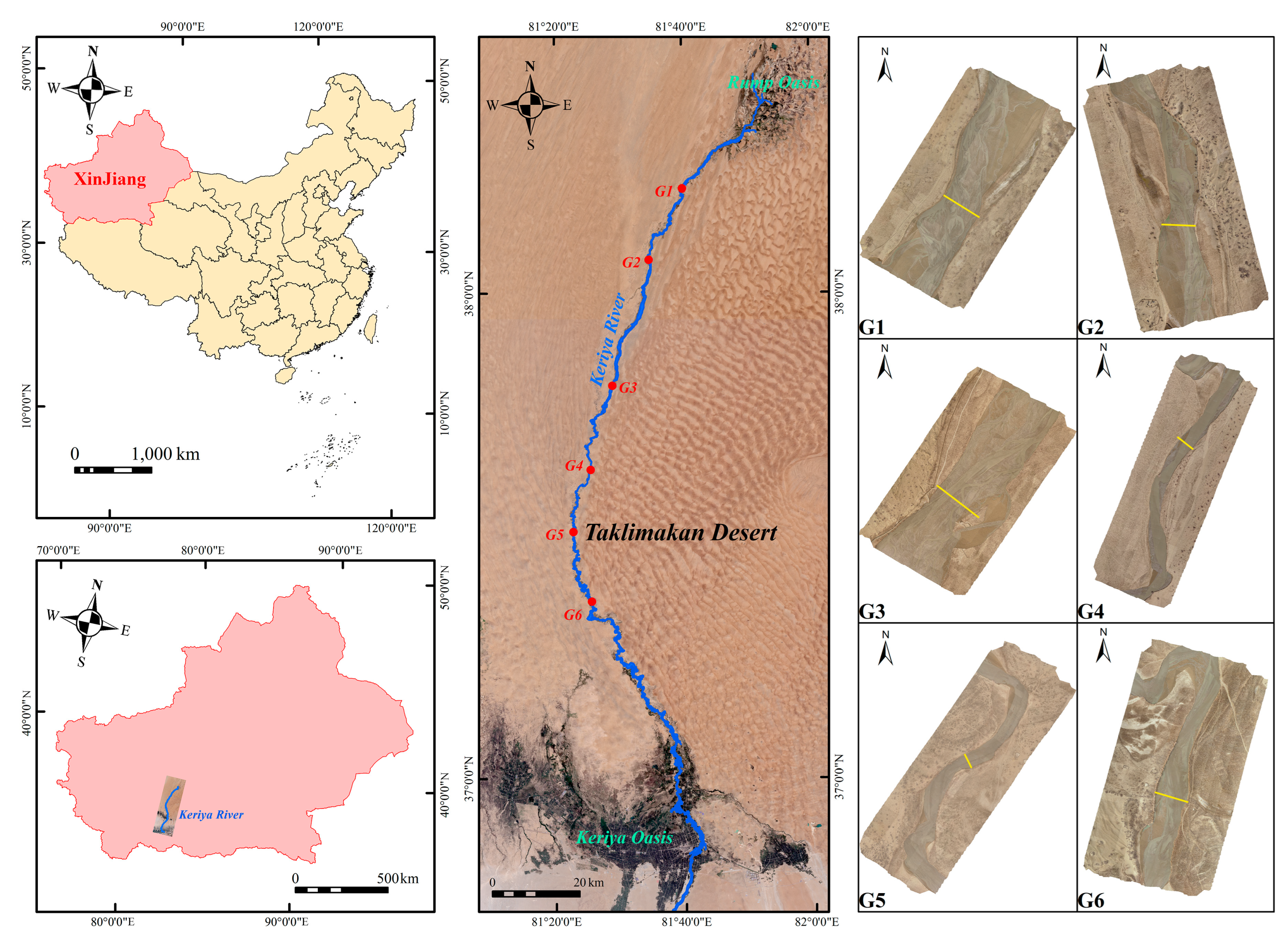
The Keriya River Basin is located in Central Asia, toward the southern edge of the Taklamakan Desert. It resides primarily within the territory of Yutian County, Hotan Region, Xinjiang, and is a typical arid inland river basin. The river originates from the north slope of Kunlun Mountain; it meanders from south to north and penetrates the hinterland of the Taklimakan Desert after passing through an artificial oasis in the middle reaches of Yutian, the formation of a natural oasis in Daliyabuyi at the end of the river. With a total length of 438 km and an average annual runoff of 7.61 × 10⁸ m3, it is the second largest river in the southern Tarim Basin after the Hotan. Here, only the Keriya hydrological station functions as a control station at the upstream outlet, whereas the middle and lower reaches of the river between Yutian Oasis and Daliyabuyi Natural Oasis are still unmonitored due to their complex topographical location, harsh environment, and lack of accessibility; therefore, runoff information is scarce.
Here, six typical river sections were selected in the middle and lower reaches of the river. An overview of the geographical location of the Keriya River and the distribution of the selected cross-sections is shown in Figure 2.

2.2. Datasets

2.2.1. UAV Data

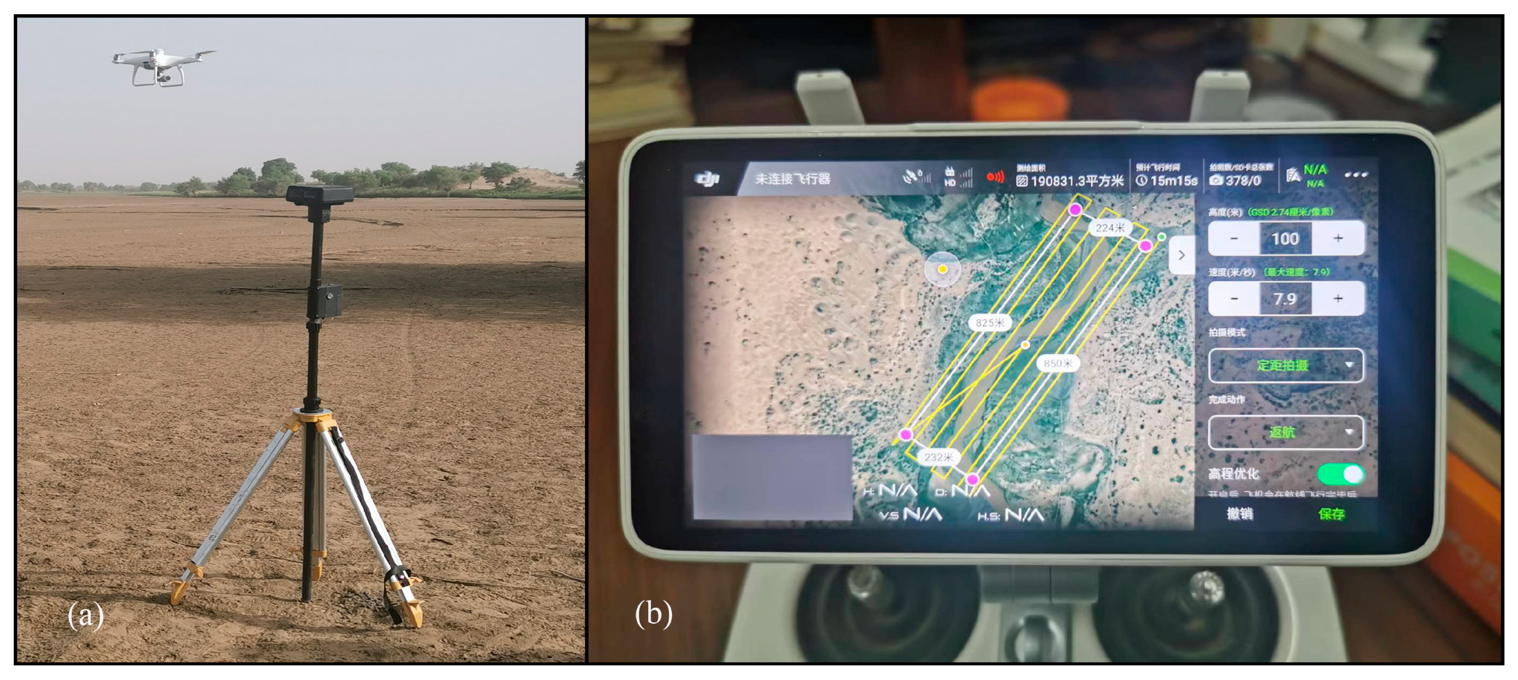
To extract more accurate river cross-sectional morphology, the DJI Phantom 4 RTK quadcopter UAV from DJI was used to conduct vertical photogrammetry during the river break, producing high-resolution DSM and DOM data (Figure 3a). The key parameters of the selected UAV equipment are shown in Table 1.
Across the six river cross-sections selected to represent the middle and lower reaches of the Keriya River, the terrain remains relatively flat, allowing for simpler field measurements of the water depth and flow rates. Representative cross-sections were taken as references, and the aerial survey area was defined by extending 250 to 300 m up- and downstream of the river. When conducting the survey, the delineated aerial area KML file was imported into the flight control software, which automatically planned the survey route (Figure 3b). To meet the resolution requirements of the UAV aerial survey images, the flight height was 100 m, considering the size of the planned aerial survey area, the actual subsurface within the survey area (mountain, tree height, etc.), and the maximum flight time that can be supported by battery power. The side and longitudinal overlap rates of the UAV aerial survey images were set to 70% and 80%, respectively, to ensure sufficient intersection of adjacent aerial survey photos and improve the image stitching quality. The UAV flight control parameters for each section are shown in Table 2.
Previous results (e.g., Zhang [48]) have shown that at a UAV aerial survey height of 50–100 m, the average image relative position error in the horizontal and vertical directions was ±0.51 and ±4.39 cm, respectively; thus, the measurement accuracy of the UAV image under the flight control system could reach the centimeter level, meeting the demand of this study. Pairs of image control points were evenly laid along both sides of the river across the aerial survey area to further improve the absolute elevation accuracy of DSM due to magnetic field interference and UAV hardware issues. The layout and style are shown in Figure 4a,c, respectively. The precise geographic coordinates and elevation of each image control point were measured with professional measuring equipment and used to correct the absolute elevation of UAV aerial survey images (Figure 4b).
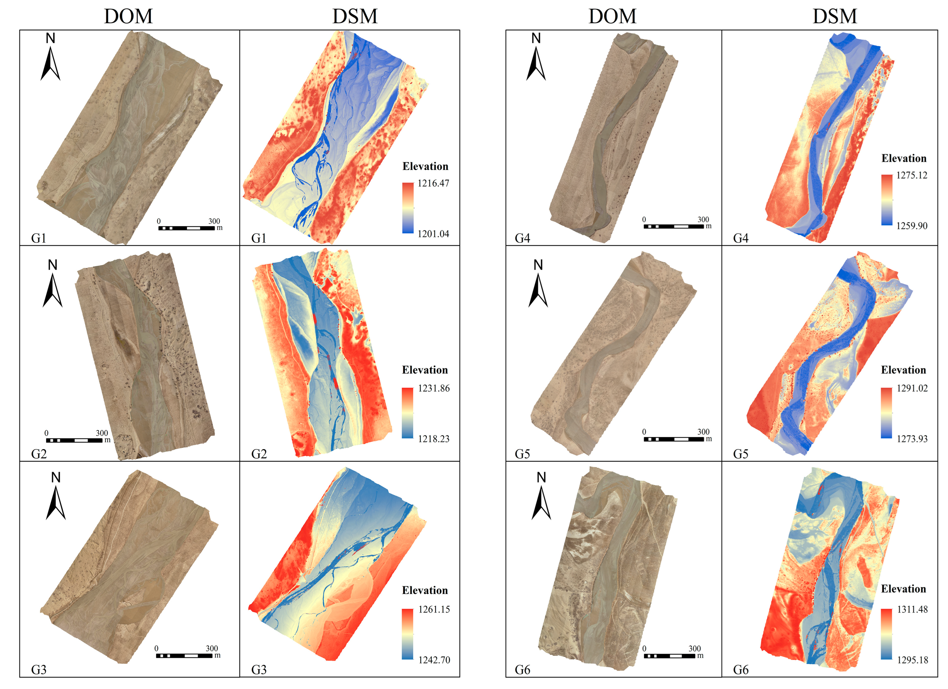
Following the UAV aerial survey, DJI Terra 3.4.4 was used to stitch the images, import the coordinates of the actual image control points, encrypt the 3D point cloud, and generate a high-precision DOM and DSM of the survey area. The DOM was used to determine the river type, distinguish the river bank boundaries, judge the vegetation cover and gravel distribution along the lower bedding surface near the river cross-section, and provide a basis for the selection of flow roughness parameters in the latter cross-section calculations; whereas the DSM was used to obtain the cross-sectional and longitudinal section elevation changes, and calculate the hydraulic radius and gradient. The DOM and DSM of each river section are shown in Figure 5.

2.2.2. Ground Measured Data

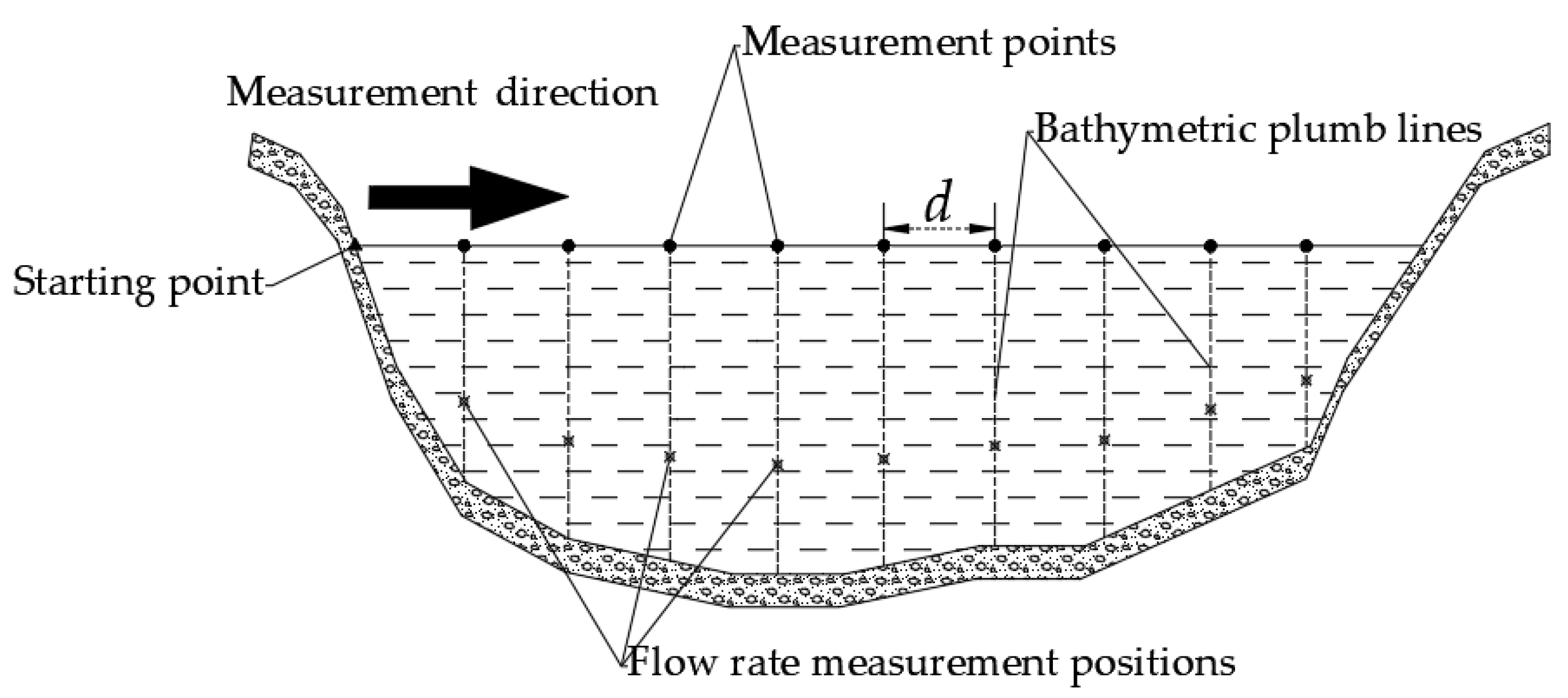
Field measurements of the water depth and flow rates were performed in selected representative cross-sections during river incoming water hours, and the measured data were compared with the derived inversion river flow rates to evaluate the method (Figure 6). The measuring points were set at equal intervals (d) along the sections, and the water depth and the flow rate were measured at 0.6 times the depth of the water at each point with portable flowmeters. Furthermore, an infrared distance meter was used to check the starting distance of each measuring point, ensuring that the distance between adjacent measuring points was equal and that the measuring section was always perpendicular to the incoming water direction.
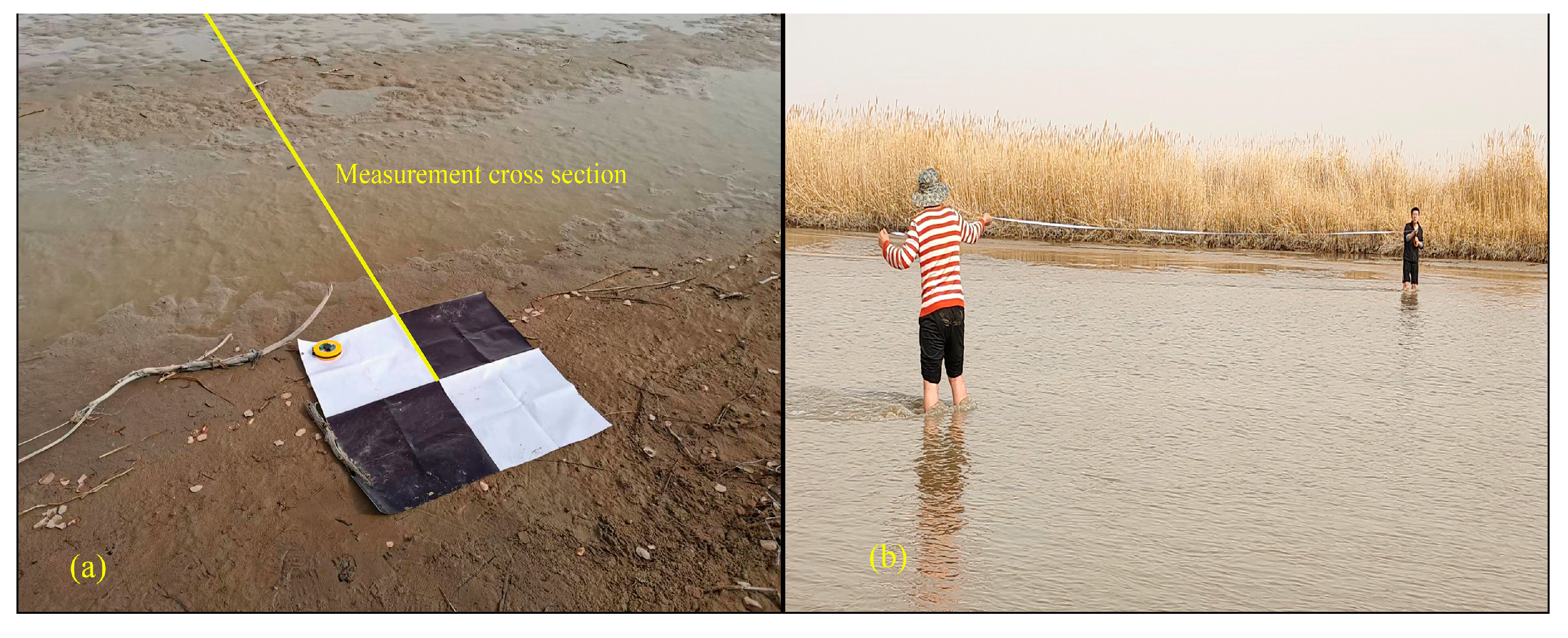
The section indicator tag was placed at the start point of the measured section so the location of the section could be visible in the remote sensing image, ensuring that the DSM location of the measured and the UAV DSM section location were appropriately linked (Figure 7a). Figure 7b shows researchers conducting water depth and flow rate measurements.

2.3. Flow Calculations

2.3.1. Low-Altitude Remote Sensing Inversion Flow–Manning’s Formula

Manning’s formula is an empirical equation for calculating unpressurized water flow, and was established based on the Chézy formula (Chézy, 1769; Equation (1)):
v = C R 1 / 2 J 1 / 2
where v is the average flow rate of the section; C is the Chézy coefficient, which reacts to the comprehensive effect of boundary conditions on water flow; R is the hydraulic radius, defined as the ratio of sectional area to the wet perimeter (i.e., is related to the sectional shape); and J is the hydraulic gradient.
As most of the natural river flow is turbulent flow within the resistance square area, the common method of calculating the Chézy coefficient is the Manning method (Equation (2)):
C = 1 n R 1 / 6
where C is the Chézy coefficient; n is the roughness, indicating the roughness of the river bed surface; and R is the hydraulic radius.
Last, the section flow estimate was obtained by associating Equations (1) and (2), as shown in Equation (3) [49]:
Q g = v × A = 1 n R 2 / 3 J 1 / 2 A  
where Qg is the flow calculated according to the Manning formula; v is the average flow rate of the section; and A is the area of the cross-section.
Accordingly, Manning’s formula involves four parameters: the cross-sectional area of the river below the water surface to the extent of inundation; the hydraulic radius coefficient characterizing the shape of the section, equal to the ratio of sectional area to wet perimeter; roughness, corresponding to the resistance of the river groove to water flow; the hydraulic gradient equal to the ratio of the amount of head loss to the distance along the flow direction of the river; and the head loss of natural rivers, as expressed by the change in the water surface elevation. Here, the topographic and water surface variation data required to calculate the hydraulic gradient were extracted from the UAV-derived DSM whereas the water cross-sectional area and hydraulic radius were obtained by calibrating the water level line in AutoCAD following the determination of the river cross-sectional geometry, whereas the roughness parameters were selected by analyzing the DSM and DOM data, field surveys, observations of riverbank types, beach vegetation coverage, and comparisons with the “Natural River Roughness Value Table” [50].

2.3.2. Actual Flow Measurement–Flow Rate-Area Method

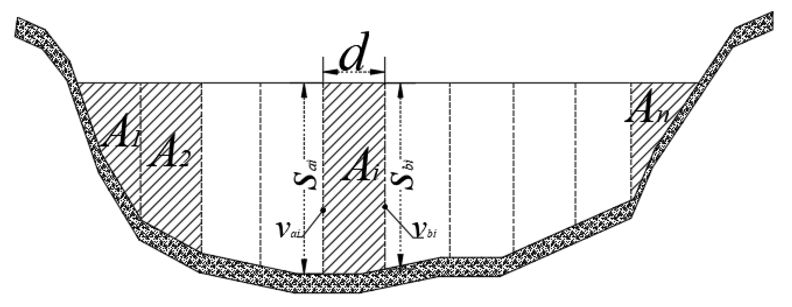
The measured flow was calculated according to the flow rate area method, as shown in the Figure 8 schematic.
Based on the water depth and flow velocity measurement method described in Section 2.2.2, after obtaining the water depth at each measurement point of the cross-section, and the flow rate 0.6 times the water depth, the river cross-section flow was calculated according to Equations (4) and (5):
Q s = Q 1 + Q 2 + Q i + Q n i = 1 , 2 , 3 , n ,
Q i = v i ¯ × A i = v a i + v b i 2 × s a i + s b i × d 2 i = 1 , 2 , 3 , n ,  
where Qs is the measured flow of the whole section; Qi is the measured flow of the ith subsection. In the subsections, d indicates the distance between adjacent bathymetry points; Ai is the area of the ith subsection surrounded by adjacent bathymetric plumbline and water surface lines; Sai indicates the water depth on the left side of the ith subsection; Sbi indicates the water depth on the right side of the ith subsection; vai is the flow rate on the left side of the ith subsection; vbi is the flow rate on the right side of the ith subsection; and v i ¯ is the average flow rate of the ith subsection.

2.4. Evaluation Methodology

To evaluate the capacity and reliability of the proposed method, RA and RMSE were chosen as the accuracy evaluation methods (Equations (6) and (7)):
R A = Q g Q s Q s ,
R M S E = 1 n Q g Q s 2 ,  
where Qg is the flow calculated according to the Manning formula and n is the total number of calculations. Here, RA (i.e., the percentage of absolute error) was used to evaluate the differences between the estimated and measured flow in a single section whereas RMSE analyzed the overall method reliability. Based on the findings of a previous study [43], an RA threshold value of 20% was established here, where only a relative precision <20% was considered reliable.

3. Results

3.1. Low-Altitude Remote Sensing Inversion

3.1.1. Hydraulic Gradient

Hydraulic gradient calculations rely on the support of river longitudinal elevation data, whereas the accurate recording of topographic information via UAV data captured subtle changes along the river longitudinal section in this study. Here, the measured river cross-section was in the middle position and extended by 250 m up- and downstream for the hydraulic gradient extraction river section. Elevation values of the upstream and downstream midpoint cross-sections were extracted, differences were calculated, and the ratio of this difference to the corresponding up- and downstream river length was used here as the hydraulic gradient results. The up- and downstream elevations, spacing, and hydraulic gradients of each cross-section are shown in Table 3. Because the selected river cross-sections are in the middle and lower reaches of the Keriya River, which itself is in the gentle sloping hinterlands of the Taklimakan Desert, the derived hydraulic gradients were considered consistent with the true topography.

3.1.2. Hydraulic Radius

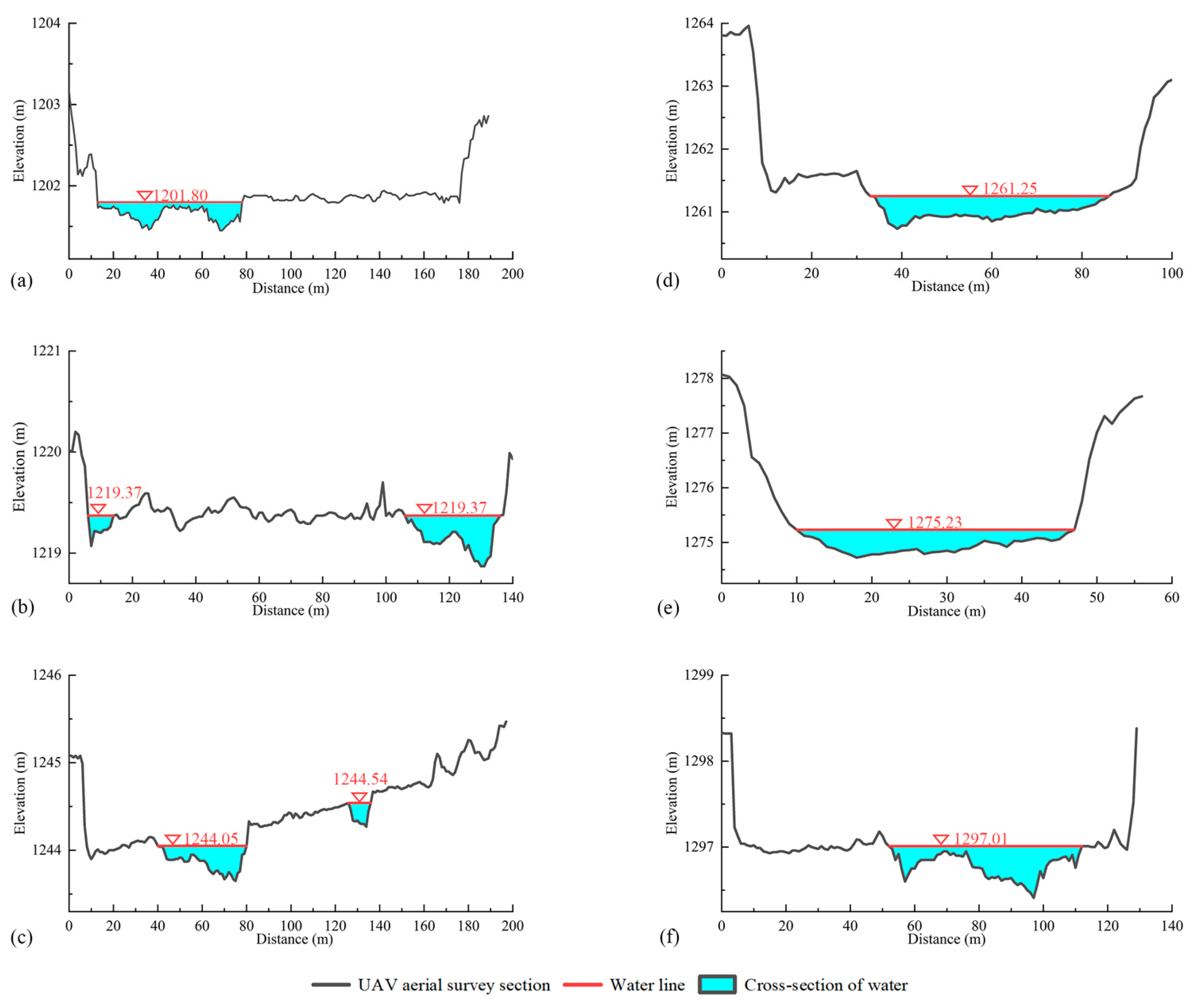
The hydraulic radius responded to the water transfer capacity of the overflow cross-section and was closely related to the cross-section shape. Here, UAV DSM-derived cross-section elevation data were imported into AutoCAD and water levels during actual cross-section measurements were marked for accuracy comparisons with actual flow data. The generated river cross-sections are shown in Figure 9. After measuring the overwater sectional area and wet perimeter, the ratio between the two was used to obtain the hydraulic radius (Table 4).

3.1.3. Roughness

Roughness corresponds to the obstructive effect of the river groove on water flow and is commonly empirically defined in existing studies [51,52]. Here, based on UAV-acquired images of the study area, the river section surrounding topography and vegetation information, including mudflat growth, the sand and gravel grain size of the river bottom, and the type of bank berm, were analyzed to obtain the roughness values against the Natural River Roughness Table. The selected section of the Keriya River maintains a wide and shallow riverbed composed of clay and fine sand, with little to no gravel. In addition, the width of the water surface at the flood level is substantially >30 m during the annual flood period. Referring to the requirements of the Natural River Roughness Table, the final roughness of each section was reported as 0.03.

3.1.4. Flow

The parameters required to estimate the flow using Manning’s formula were obtained using the steps in Section 3.1.1 Section 3.1.2 and Section 3.1.3, and the results of the low-altitude remote sensing inversion river flow calculations are shown in Table 5.

3.2. Section Measured Flow Results

To verify the feasibility of the UAV low-altitude remote sensing inversion method for river flow, field measurements of the water depth and flow velocity were collected at selected representative cross-sections during river incoming water hours, and the measured flow was calculated, the results of which are shown in Table 6.

3.3. Accuracy Analyses

Here, 20% of the measured flow was the maximum allowable error when evaluating the calculated flow accuracy. Table 7 displays the measured flow and calculated flow according to Manning’s formula, the absolute error, and the RA for the six cross-sections, respectively. The RA of G2–G5 was small, whereas that for G1 and G6 was relatively higher (14.37% and 17%, respectively) but still fell below the threshold.
Overall, the average RA of the calculated and measured flows was ~8.49%, indicating the relatively high capacity of the methods. In particular, the large error observed in G1 was likely due to the wide surface of the water and shallow depth at this location, where small fluctuations in the riverbed have more obvious impacts on the flow calculation results. Furthermore, G6 is in the middle reaches of the Keriya River, where the water depth is greater, and the water velocity is relatively faster; moreover, the bottom of the riverbed here is fine sandy clay, which is more prone to changes in siltation. Thus, this results in actual measurement errors.
Alternatively, the RMSE used to reflect the deviation between the measured and estimated runoff is more sensitive to extreme values. Here, the calculated RMSE was 0.59 m3·s−1, indicating a relatively small deviation between the estimated and measured runoff and the overall reliability of the implemented method.

3.4. Water Surface Width (Water Depth)–Flow Relationships

Based on the measured cross-sectional river morphology, the area and wet perimeter of the overwater cross-section at different water levels were extracted according to variable water level heights, and the corresponding flow rates were calculated via Manning’s formula. The water surface width–flow and depth–flow relationship scatterplots were drawn and the optimal curve model was selected using a nonlinear curve fitting function of OriginPro 2021 (OriginLab Corporation, Northampton, Massachusetts, USA).
For the water depth–flow scatterplots, this study analogously draws on the recommended method of the international standard to fit the water level–flow relationship and choose the power function model Allomometric 2 ( y = b x c + a ) for curve fitting [53,54]. The results showed that the coefficient of determination R2 of the fitted curves of each section reached 0.99. This indicates that the power function model Allomometric 2 applies to the fitting of water level–flow relationship curves in addition to natural river cross-sections and also applies to the fitting of water depth–flow relationship curves.
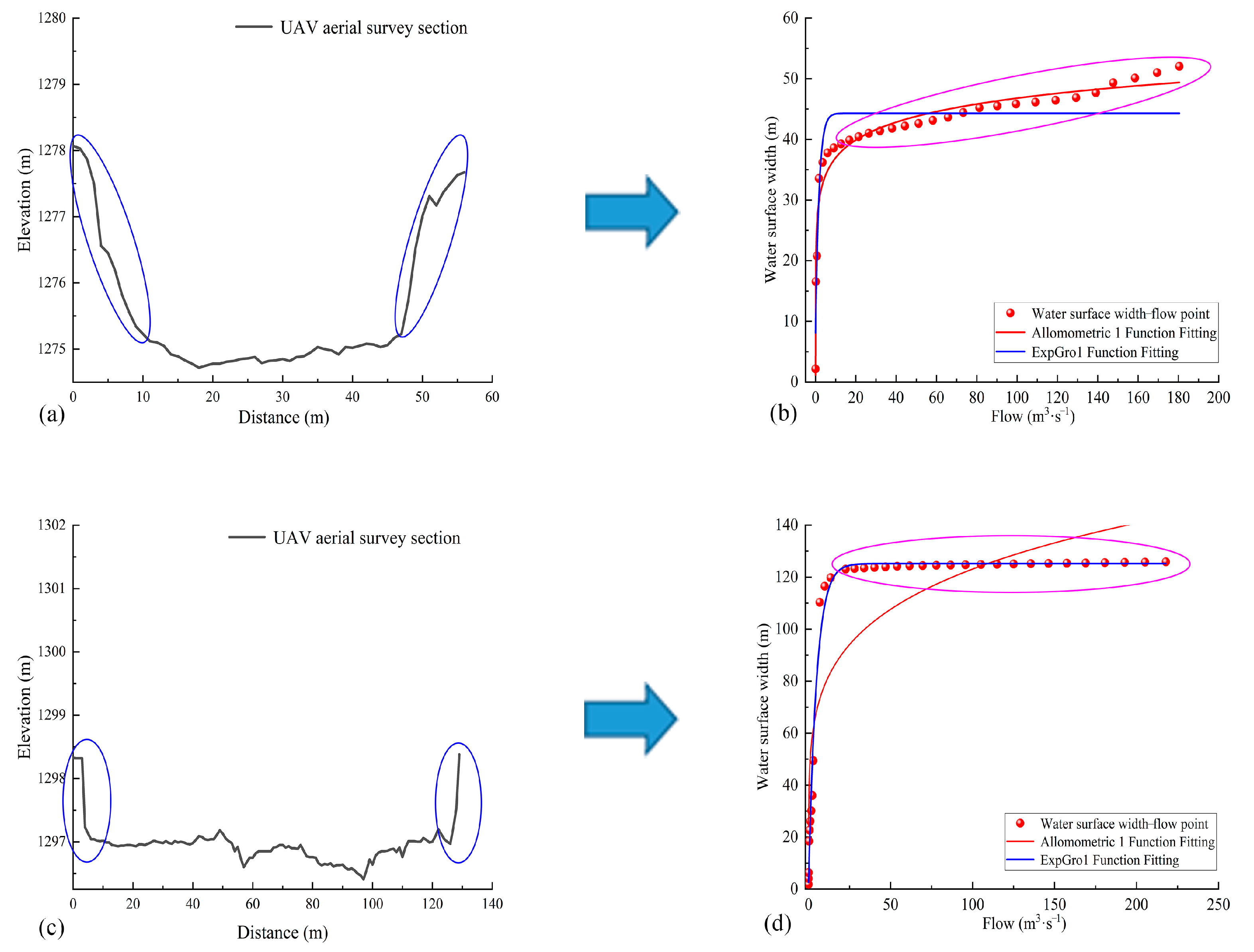
For the water surface width–flow scatterplots, this study refers to the research results of Leopold and Maddock [55,56], and two power function models such as Allomometric 1 and Allomometric 2, and three exponential function models such as ExpGro1, ExpGro2, and ExpGro3 were selected for fitting, respectively. The fitting effects of different function models were compared and analyzed. The effect of the fitting effect of the function models was correlated with the morphology of the section, as shown in Figure 10.
As shown in Figure 10a,b, when the embankments on both sides of the river cross-section are inclined, the water surface width–flow scatterplots in the corresponding high value area of the water surface width–flow scatterplots are an inclined distribution, and the fit of the power function model is better at this time. As shown in Figure 10c,d, when the embankment is vertical, the corresponding water surface width–flow scatter in the high value area of the flow is close to the horizontal distribution and the fit of the exponential function model in such cases is better.
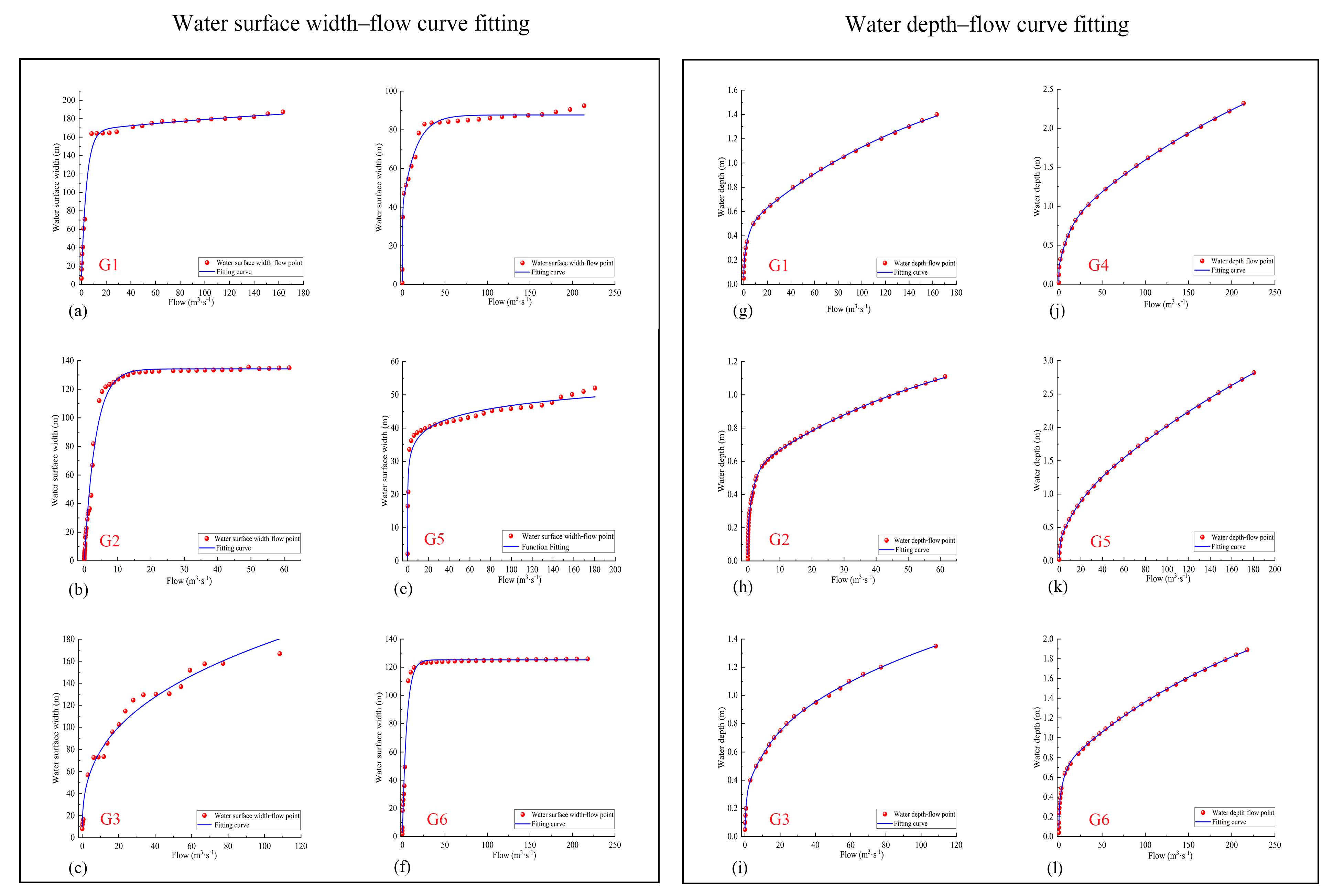
Finally, according to the morphology of each section and the characteristics of the water surface width–flow scatter distribution, the Allomometric 2 ( y = b x c + a ) model with a better fitting effect in the power function was selected to fit for the G1, G2, G4, and G6 sections. The ExpGro3 ( y = y 0 + A 1 e x / t 1 + A 2 e x / t 2 + A 3 e x / t 3 ) model with a better fitting effect in the exponential function was chosen for the G3 and G5 sections. The water surface width (water depth)–flow relationship curves for each section are shown in Figure 11, whereas the curve–fitting relationships and corresponding R2 values are shown in Table 8 and Table 9.
According to the surface width (water depth)–flow relationship curves, flow rates that are not conducive to direct measurement can be estimated via directly available water surface width and depth for the observation of river flow. Moreover, the specific choice of surface width–flow or depth–flow relationships is determined by the studied cross-section’s morphology and different water volume periods (periods of high water volume and periods of low water volume).

3.5. Analysis of Flow Inversion Methods across Cross-Sectional Forms

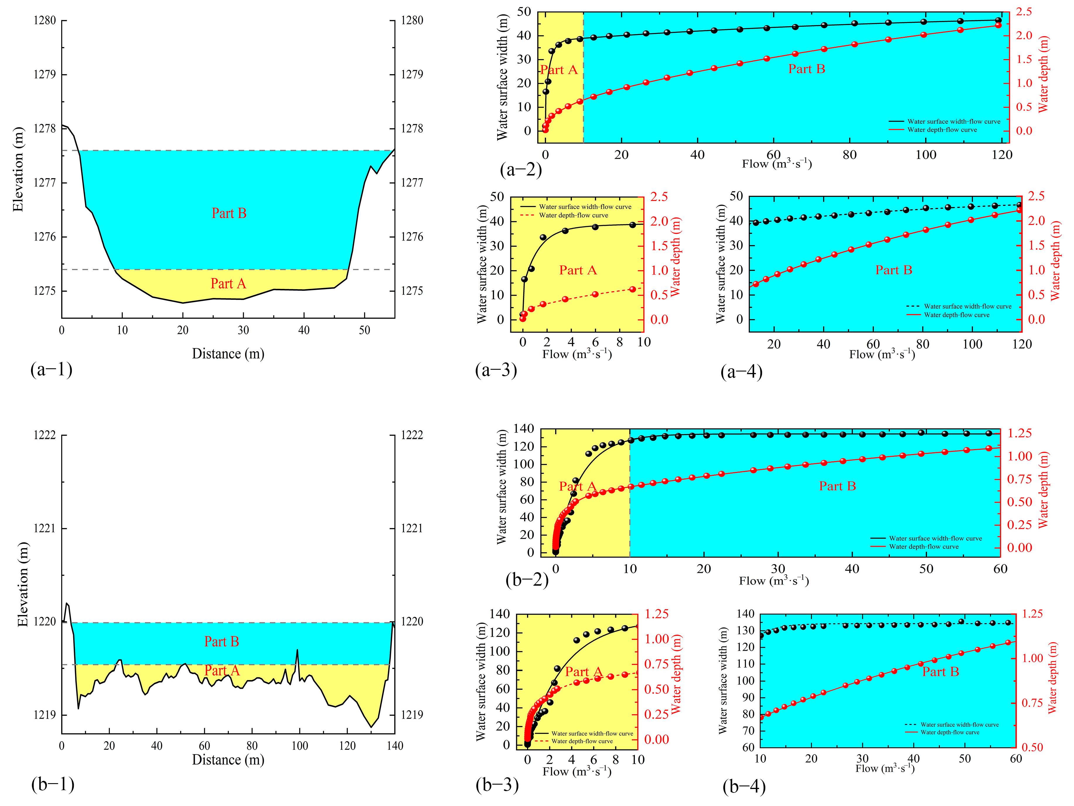
The middle and lower reaches of the Keriya River covered in this study have multiple wide and shallow riverbeds, and the morphology of the characteristics of the river cross-section varied by location. Accordingly, cross-sections were placed into two category types: gentle bottom and raised bottom. Subsequently, the flow variation and suitable flow inversion methods corresponding to the morphological characteristics of the above two river cross-sections (Figure 12) were analyzed.
Figure 12a shows that the bottom gentle type of section was “U” shaped. As the bottom of the riverbed is relatively gentle, this type of section is mostly seen at narrow river widths, where river waters are relatively concentrated, depths are greater, and the water velocity is faster. In such instances, riverbed bottoms are relatively gentle due to the scouring effect of water. This resulting cross-section bed morphology is relatively simple, and the overall water surface width (depth)–flow relationship was determined here for different water volume periods, with each flow having a unique corresponding water surface width or depth values. Only when this condition is met can the surface width (depth)–flow relationship curve be used to support estimation of the corresponding momentary flow based on the water surface width or depth.
Figure 12a Part A indicates that at lower flow rates, and when the water surface has not completely covered the riverbed bottom, the water surface width increases rapidly with increasing flow, and the difference of the water surface width during this period more clearly reflects the flow change, whereas the variation in the water depth is relatively small and does not reflect the effect of flow change as clearly. Therefore, the section flow in this period can be obtained by high-resolution remote sensing imagery or UAV aerial images of the water surface width at the section locations and estimated based on the water surface width–flow relationship curve.
Figure 12a Part B shows that during periods of higher flow, the water surface has completely covered the bottom of the riverbed, and as the flow continues to increase, the width of the water surface is limited by the embankments on both sides. Consequently, the resulting increase in flow is small and the effect of the water surface width reflecting the changes in flow during this period is less obvious. Conversely, water depth is not affected by the surrounding embankments and can thus better reflect flow changes. Thus, the periods of water depth changes are more appropriate for reflecting the effects of flow changes and based on the water depth–flow relationship curve, more accurate estimates of sectional flow can be obtained through simple water depth measurements.
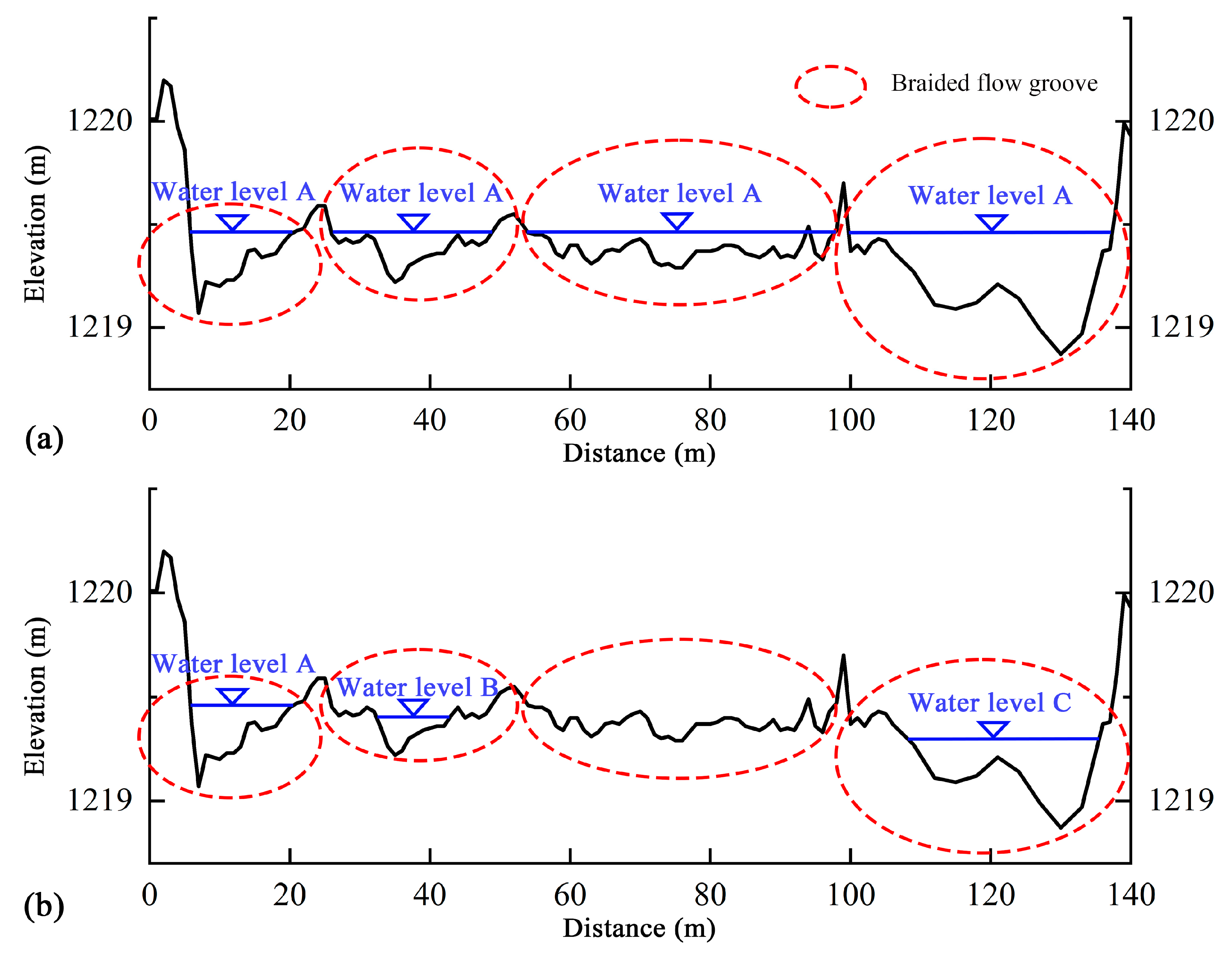
The bottom protrusion type section in Figure 12b, which has a non-negligible protrusion at its section bottom, is mostly seen in downstream grooves, where the riverbed is wider and the water is relatively dispersed, and these dispersed water flows are called “braided flow.” At low water volumes and shallow depths, the braided flow is more easily formed. Ideally, the water flow in the braided flow period is evenly distributed within each “braided flow groove”, whereas the surface height of each groove remains equal (Figure 13a). The overall water surface width (water depth)–flow relationship of the cross-section in this state was uniquely determined, and the correlation between the water surface width (water depth) and flow was analyzed for the entire river cross-section. The resulting effect of differences in the water surface width on flow variation during this period was more obvious compared to the water depth (Figure 12b, Part A).
However, in this study, it was found that the actual water passage in the braided flow groove during the corresponding flow period may differ from the ideal state (Figure 13b). Due to the influence of various factors, including the topography, slope, and water volume, water will randomly flow in ≥1 braided flow grooves with different cross-sectional patterns, although not necessarily in all braided grooves. Because the water body in each braided flow groove is not connected, the elevation of the water surface in each braided flow groove also varies. The above factors lead to the overall water surface width (water depth)–flow relationship of the section being less unique, with several water surface widths (depths) corresponding to the same or different flow patterns.
Therefore, during the actual analysis of such cross-sectional braid flow water surface width (depth)–flow change relationships, cross-sections must be broken down into several braided flow grooves, each functioning as an independent cross-section (i.e., not the overall river cross-section), for which a water surface width (depth)–flow relationship curve can be derived. Following decomposition, each braided flow groove was approximated as a “V”- or “W”-shaped section, where the change in the water surface width for each groove can more clearly reflect the flow variation during this period. The resulting water surface width in each braided flow groove of the section can be obtained by high-resolution remote sensing or UAV imagery, and the resulting flow can be estimated based on the relationship curve of the water surface width and flow for each groove. Last, the flow of each braided groove can be summated to reveal the total cross-sectional flow.
All braided flow grooves are filled with water in larger volumes (Figure 12b, Part B); therefore, when the river is full of grooves, and the water surface completely covers the protrusion at the bottom of the riverbed, the randomness of the overwater situation in the braided flow grooves no longer needs to be considered, and the overall water surface width (depth)–flow relationship of the section can be uniquely determined similarly to that for gently sloping sections, where the width of the water surface is limited by the embankment on both sides. Here, the increase is less obvious and cannot better reflect flow changes, whereas the water depth can better reflect such changes, as it remains unaffected by the embankments on either side of the river. Therefore, the cross-sectional flow during this period can also be estimated by simple bathymetry measurements at the deepest position of the cross-section and based on the overall bathymetry–flow relationship curve of the cross-section.

4. Discussion

4.1. Method Strengths

Over recent decades, scholars from various countries have extracted river cross-section information, largely based on various types of high-altitude satellite remote sensing data; however, such methods maintain limitations that remain to be resolved. First, the spatial resolution of high-altitude satellite imagery is often limited. For example, the spatial resolution of Landsat 8 is 30 m across the visible and IR bands, whereas that of Sentinel-2A is 10 m across the visible wavelengths. Here, the analyzed width of the Keriya River water surface is only a few tens of meters during periods of low water volume; thus, the resulting width of the water surface would only be 2 to 3 Landsat pixels or 8–9 Sentinel-2A image pixels, far below the spatial resolutions required to satisfy the requirements for extracting water surface information across the river section. Second, the quality of remote sensing images is commonly affected by cloud cover, and when coupled with long revisit times of numerous satellites, it is difficult to achieve information at high temporal resolutions for any point of a river section.
The extraction of river cross-section information through UAV-based low-altitude photogrammetry does not have these problems. First, the relatively low flight altitudes mean that cloud will rarely be an issue, ensuring a comprehensive dataset at high resolutions. Here, the DJI Phantom 4 RTK quadrotor UAV used can achieve a ground resolution of 2.74 cm when the flight height is set to 100 m, thus successfully meeting the demand for information extraction of narrower river sections, and water surface widths when water volumes are low. Simultaneously, by evenly laying image control points on either side of the river groove and using RTK to obtain coordinates and elevation information of the said control points, the horizontal position and absolute elevation accuracy of the aerial UAV survey images can be effectively ensured to guarantee the fitting effect of the river cross-section. Furthermore, UAV equipment is small, light, easy to transport, convenient, and provides rapid data acquisition, among other advantages; thus, it can realize information from the river cross-section with substantial speed, which highlights the marked advantages for the extraction of small and medium river cross-sections in arid areas through the methods used here.

4.2. Method Limitations

First, controlling UAV volume and weight are essential components for transport and functionality. In particular, smaller sizes and lower weights often indicate weaker UAV endurance. Namely, UAV flight batteries must provide sufficient power for normal takeoff, landing, hovering, and other flight commands under strict control of volume and weight, which determines the short endurance and thus limits the flight range of the UAV. Furthermore, it has a relatively small UAV volume and weaker wind resistance. Moreover, the aircraft can be more easily blocked by objects, such as mountains and trees midflight; thus, there are certain requirements for flight area environments that must be met.
Second, because the UAV selected for this study was equipped with a visible wavelength camera, it could not penetrate the surface of the water (especially water bodies of sediment) to apply the inversion method for deriving river flow [57]. Therefore, only rivers without water or during dry periods should be selected to conduct UAV aerial surveys to obtain riverbed section morphological estimates more precisely. Furthermore, the real shape of the underwater river cross-section was inverted by selecting LIDAR-equipped UAVs or bathymetric vessels to measure the study cross-section.

5. Conclusions

  • Low-altitude remote sensing by UAV was employed to monitor riverbed characteristics, and, with classical hydraulics equations, river flow from ungauged basins in the desert hinterland rivers of the middle and lower reaches of the Keriya River, northwest China, was derived using a UAV inversion method. Consequently, this is a novel approach to current limitations when estimating runoff for small- and medium-sized inland rivers.
  • RA and RMSE were used to evaluate the applicability and reliability of the low-altitude remote sensing inversion method, revealing averages of 8.49% (ranging 3.26–17.00%; which fell within the allowable error range) and 0.59 m3·s−1, respectively, supporting the functionality of the proposed method within the study area.
  • According to the water surface width (water depth)–flow relationship curve of each section, combined with the morphological characteristics of the section, different water volume periods were selected, the optimal water surface width–flow relationship or water depth–flow relationship was selected, and a method for estimating river flow was proposed to provide a reference for the estimation of small- and medium-sized river runoff.

Author Contributions

Conceptualization, M.Z. and Y.G.; formal analysis, N.W. and Y.B.; investigation, M.Z., N.W., X.W., Y.B., and H.W.; methodology, M.Z., Y.G. and X.W.; visualization, M.Z. and N.W.; writing—original draft, M.Z. and Y.G.; writing—review and editing, M.Z. and Y.G. All authors have read and agreed to the published version of the manuscript.

Funding

This research was funded by the National Natural Science Foundation of China (Grant Nos. U1703237; 41961003).

Institutional Review Board Statement

Not applicable.

Informed Consent Statement

Not applicable.

Data Availability Statement

The data presented in this study are available on request from the corresponding author.

Acknowledgments

The authors thank the National Natural Science Foundation of China.

Conflicts of Interest

The authors declare no conflict of interest.

References

  1. Yang, S. Ecohydrological Models: Introduction and Application; Science Press: Beijing, China, 2012; pp. 1–17. [Google Scholar]
  2. Escartın, J.; Aubrey, D.G. Flow structure and dispersion within algal mats. Estuar. Coast. Shelf Sci. 1995, 40, 451–472. [Google Scholar] [CrossRef]
  3. Alsdorf, D.E.; Lettenmaier, D.P. Tracking fresh water from space. Science. 2003, 301, 1491–1494. [Google Scholar] [CrossRef] [PubMed] [Green Version]
  4. Bjerklie, D.M.; Ayotte, J.D.; Cahillane, M.J. Simulating Hydrologic Response to Climate Change Scenarios in Four Selected Watersheds of New Hampshire; U.S. Geological Survey Scientific Investigations Report; U.S. Geological Survey: Reston, VA, USA, 2015.
  5. Hirpa, F.A.; Hopson, T.M.; De Groeve, T.; Brakenridge, G.; Gebremichael, M.; Restrepo, P.J. Upstream satellite remote sensing for river discharge forecasting: Application to major rivers in South Asia. Remote Sens. Environ. 2013, 131, 140–151. [Google Scholar] [CrossRef]
  6. LeFavour, G.; Alsdorf, D. Water slope and discharge in the Amazon River estimated using the shuttle radar topography mission digital elevation model. Geophys. Res. Lett. 2005, 32, 404–405. [Google Scholar] [CrossRef] [Green Version]
  7. Jung, H.C.; Hamski, J.; Durand, M.; Alsdorf, D.; Hossain, F.; Lee, H.; Hossain, A.K.M.A.; Hasan, K.; Khan, A.S.; Hoque, A.Z. Characterization of complex fluvial systems using remote sensing of spatial and temporal water level variations in the Amazon, Congo, and Brahmaputra Rivers. Earth Surf. Process. Landf. 2010, 35, 294–304. [Google Scholar] [CrossRef]
  8. Smith, L.C.; Isacks, B.L.; Forster, R.R.; Bloom, A.L.; Preuss, I. Estimation of discharge from braided glacial rivers using ERS-1 Synthetic-Aperture Radar—First results. Water Resour. Res. 1995, 31, 1325–1329. [Google Scholar] [CrossRef]
  9. Smith, L.C.; Isacks, B.L.; Bloom, A.L.; Murray, A.B. Estimation of Discharge from Three Braided Rivers Using Synthetic Aperture Radar Satellite Imagery: Potential Application to Ungaged Basins. Water Resour. Res. 1996, 32, 2021–2034. [Google Scholar] [CrossRef]
  10. Xu, K.; Zhang, J.; Watanabe, M.; Sun, C. Estimating river discharge from very high-resolution satellite data: A case study in the Yangtze River, China. Hydrol. Process. 2004, 18, 1927–1939. [Google Scholar] [CrossRef]
  11. Pavelsky, T.M. Using width-based rating curves from spatially discontinuous satellite imagery to monitor river discharge. Hydrol. Process. 2014, 28, 3035–3040. [Google Scholar] [CrossRef]
  12. Gleason, C.J.; Wang, J. Theoretical basis for at-many-stations hydraulic geometry. Geophys. Res. Lett. 2015, 42, 7107–7114. [Google Scholar] [CrossRef]
  13. Zhang, J.; Xu, K.; Watanabc, M. Estimation of river discharge using very high-resolution satellite data in Yangtze River. In Proceedings of the International Symposium on Remote Sensing, Sokcho, Korea, 24–28 June 2002; pp. 728–733. [Google Scholar]
  14. Getirana, A.C.V.; Peters-Lidard, C. Estimating water discharge from large radar altimetrydatasets. Hydrol. Earth Syst. Sci. 2013, 17, 923. [Google Scholar] [CrossRef] [Green Version]
  15. Papa, F.; Durand, F.; Rossow, W.B.; Rahman, A.; Bala, S.K. Satellite altimeter-derived monthly discharge of the Ganga-Brahmaputra River and its seasonal to interannual variations from 1993 to 2008. J. Geophys. Res. Earth Surf. 2010, 115, 13. [Google Scholar] [CrossRef] [Green Version]
  16. Biancamaria, S.; Lettenmaier, D.P.; Pavelsky, T.M. The SWOT Mission and Its Capabilities for Land Hydrology. Surv. Geophys. 2016, 37, 307–337. [Google Scholar] [CrossRef] [Green Version]
  17. Pavelsky, T.M.; Durand, M.T.; Andreadis, K.M.; Beighley, R.E.; Paiva, R.C.D.; Allen, G.H.; Miller, Z.F. Assessing the potential global extent of SWOT river discharge observations. J. Hydrol. 2014, 519, 1516–1525. [Google Scholar] [CrossRef]
  18. Gosling, S.N.; Arnell, N.W. Simulating current global river runoff with a global hydrological model: Model revisions, validation, and sensitivity analysis. Hydrol. Process. 2011, 25, 1129–1145. [Google Scholar] [CrossRef]
  19. Widén-Nilsson, E.; Halldin, S.; Xu, C. Global water-balance modelling with WASMOD-M: Parameter estimation and regionalisation. J. Hydrol. 2007, 340, 105–118. [Google Scholar] [CrossRef]
  20. Rawlins, M.A.; Lammers, R.B.; Frolking, S.; Vorosmarty, C.J. Simulating pan-Arctic runoff with a macro-scale terrestrial water balance model. Hydrol. Process. 2003, 17, 2521–2539. [Google Scholar] [CrossRef]
  21. Oki, T.; Nishimura, T.; Dirmeyer, P. Assessment of Annual Runoff from Land Surface Models Using Total Runoff Integrating Pathways (TRIP). J. Meteorol. Soc. Jpn. Ser. II 1999, 77, 235–255. [Google Scholar] [CrossRef] [Green Version]
  22. Durand, M.; Gleason, C.J.; Garambois, P.A.; Bjerklie, D.; Smith, L.C.; Roux, H.; Rodriguez, E.; Bates, P.D.; Pavelsky, P.M.; Monnier, J.; et al. An intercomparison of remote sensing river discharge estimation algorithms from measurements of river height, width, and slope. Water Resour. Res. 2016, 52, 4527–4549. [Google Scholar] [CrossRef] [Green Version]
  23. Birkinshaw, S.J.; Moore, P.; Kilsby, C.G.; O’Donnell, G.M.; Hardy, A.J.; Berry, P.A.M. Daily discharge estimation at ungauged river sites using remote sensing. Hydrol. Process 2014, 28, 1043–1054. [Google Scholar] [CrossRef]
  24. Birkinshaw, S.J.; O'Donnell, G.M.; Moore, P.; Kilsby, C.; Fowler, H.; Berry, P.A.M. Using satellite altimetry data to augment flow estimation techniques on the Mekong River. Hydrol. Process. 2010, 24, 3811–3825. [Google Scholar] [CrossRef]
  25. Gleason, C.J.; Garambois, P.-A.; Durand, M.T. Tracking River Flows from Space. Earth Space Sci. News 2017, 7, 98. [Google Scholar] [CrossRef]
  26. Andreadis, K.M.; Clark, E.A.; Lettenmaier, D.P.; Alsdorf, D.E. Prospects for river discharge and depth estimation through assimilation of swath-altimetry into a raster-based hydrodynamics model. Geophys. Res. Lett. 2007, 34, 403. [Google Scholar] [CrossRef] [Green Version]
  27. Gleason, C.J.; Smith, L.C. Toward global mapping of river discharge using satellite images and at-many-stations hydraulic geometry. Proc. Natl. Acad. Sci. USA 2014, 111, 4788–4791. [Google Scholar] [CrossRef] [PubMed] [Green Version]
  28. Garambois, P.-A.; Monnier, J. Inference of effective river properties from remotely sensed observations of water surface. Adv. Water Resour. 2015, 79, 103–120. [Google Scholar] [CrossRef]
  29. Ling, F.; Cai, X.; Li, W.; Xiao, F.; Li, X.; Du, Y. Monitoring river discharge with remotely sensed imagery using river island area as an indicator. J. Appl. Remote Sens. 2012, 6, 563–564. [Google Scholar] [CrossRef]
  30. Watts, A.C.; Ambrosia, V.G.; Hinkley, E.A. Unmanned Aircraft Systems in Remote Sensing and Scientific Research: Classification and Considerations of Use. Remote Sens. 2012, 4, 1671–1692. [Google Scholar] [CrossRef] [Green Version]
  31. Colomina, I.; Molina, P. Unmanned aerial systems for photogrammetry and remote sensing: A review. ISPRS J. Photogramm. Remote Sens. 2014, 92, 79–97. [Google Scholar] [CrossRef] [Green Version]
  32. Lee, S.; Choi, Y. Topographic Survey at Small-scale Open-pit Mines using a Popular Rotary-wing Unmanned Aerial Vehicle (Drone). J. Korean Soc. Rock Mech. 2015, 25, 462–469. [Google Scholar]
  33. Cho, S.-J.; Bang, E.-S.; Kang, I.-M. Construction of Precise Digital Terrain Model for Nonmetal Open-pit Mine by Using Unmanned Aerial Photograph. Econ. Environ. Geol. 2015, 48, 205–212. [Google Scholar] [CrossRef]
  34. Neugirg, F.; Stark, M.; Kaiser, A.; Vlacilova, M.; Della Seta, M.; Vergari, F.; Schmidt, J.; Becht, M.; Haas, F. Erosion processes in calanchi in the Upper Orcia Valley, Southern Tuscany, Italy based on multitemporal high-resolution terrestrial LiDAR and UAV surveys. Geomorphology 2016, 269, 8–22. [Google Scholar] [CrossRef]
  35. Vivoni, E.R.; Rango, A.; Anderson, C.A.; Pierini, N.A.; Schreiner-McGraw, A.P.; Saripalli, S.; Laliberte, A.S. Ecohydrology with unmanned aerial vehicles. Ecosphere 2014, 5, 1–14. [Google Scholar] [CrossRef] [Green Version]
  36. Li, D.; Chen, X.; Cai, X. Spatial information techniques in rapid response to Wenchuan Earthquake. J. Remote Sens. 2008, 12, 841–851. [Google Scholar]
  37. Wang, P.; Yang, S.; Wang, J.; Pan, T.; Zhang, S.; Gong, T. Discharge estimation with hydraulic geometry using unmanned aerial vehicle and remote sensing. Shuili Xuebao 2020, 51, 492–504. [Google Scholar] [CrossRef]
  38. Lewin, J.; Gibbard, P.L. Quaternary river terraces in England:forms, sediments and processes. Geomorphology 2010, 120, 293–311. [Google Scholar] [CrossRef]
  39. Yang, Z.; Wu, S.; Chen, G. River cross section survey method based on UAV and GPS-RTK. J. Suzhou Univ. Sci. Technol. 2020, 37, 65–70. [Google Scholar] [CrossRef]
  40. Yang, S.; Wang, P.; Lou, H.; Wang, J.; Zhao, C.; Gong, T. Estimating River Discharges in Ungauged Catchments Using the Slope area Method and Unmanned Aerial Vehicle. Water 2019, 11, 2361. [Google Scholar] [CrossRef] [Green Version]
  41. Lou, H.; Wang, P.; Yang, S.; Hao, F.; Ren, X.; Wang, Y.; Shi, L.; Wang, J.; Gong, T. Combining and Comparing an Unmanned Aerial Vehicle and Multiple Remote Sensing Satellites to Calculate Long-Term River Discharge in an Ungauged Water Source Region on the Tibetan Plateau. Remote Sens. 2020, 12, 2155. [Google Scholar] [CrossRef]
  42. Yang, S.; Li, C.; Lou, H.; Wang, P.; Wang, J.; Ren, X. Performance of an Unmanned Aerial Vehicle (UAV) in Calculating the Flood Peak Discharge of Ephemeral Rivers Combined with the Incipient Motion of Moving Stones in Arid Ungauged Regions. Remote Sens. 2020, 12, 1610. [Google Scholar] [CrossRef]
  43. Yang, S.; Wang, P.; Wang, J.; Lou, H.; Gong, T. River flow estimation method based on UAV aerial photogrammetry. Natl. Remote Sens. Bull. 2021, 25, 1284–1293. [Google Scholar] [CrossRef]
  44. Zhao, C.; Pan, X.; Yang, S.; Liu, C.; Chen, X.; Zhang, H.; Pan, T. Measuring streamflow with low-altitude UAV imagery. Acta Geogr. Sin. 2019, 7, 1392–1408. [Google Scholar]
  45. Wufu, A.; Chen, Y.; Yang, S.; Lou, H.; Wang, P.; Li, C.; Wang, J.; Ma, L. Changes in Glacial Meltwater Runoff and Its Response to Climate Change in the Tianshan Region Detected Using Unmanned Aerial Vehicles (UAVs) and Satellite Remote Sensing. Water 2021, 13, 1753. [Google Scholar] [CrossRef]
  46. Zhao, C.; Zhang, C.; Yang, S.; Liu, C.; Xiang, H.; Sun, Y.; Yang, Z.; Zhang, Y.; Yu, X.; Shao, N.; et al. Calculating e-flow using UAV and ground monitoring. J. Hydrol. 2017, 552, 351–365. [Google Scholar] [CrossRef]
  47. Wufu, A.; Yang, S.; Chen, Y.; Lou, H.; Li, C.; Ma, L. Estimation of Long-Term River Discharge and Its Changes in Ungauged Watersheds in Pamir Plateau. Remote Sens. 2021, 13, 4043. [Google Scholar] [CrossRef]
  48. Zhang, C.; Yang, S.; Zhao, C.; Lou, H.; Zhang, Y.; Bai, J.; Zhang, Z.; Guan, Y. Topographic data accuracy verification of small consumer UAV. J. Remote Sens. 2018, 22, 185–195. [Google Scholar] [CrossRef]
  49. Sun, D.; Ding, X. Hydraulics; The Yellow River Water Conservancy Press: Zhengzhou, China, 2009; pp. 175–177. [Google Scholar]
  50. Zhao, Z.; He, J. Hydraulics, 2nd ed; TsingHua University Press: Beijing, China, 2010; pp. 176–177. [Google Scholar]
  51. Simons, D.B.; Li, R.-M.; Al-Shaikh-Ali, K.S. Flow Resistance in Cobble and Boulder Riverbeds. J. Hydraul. Div. 1979, 105, 477–488. [Google Scholar] [CrossRef]
  52. Beven, K.; Binley, A. The future of distributed models: Model calibration and uncertainty prediction. Hydrol. Process. 1992, 6, 279–298. [Google Scholar] [CrossRef]
  53. Ma, H. Application of Excel software in the temporary curve of water level flow relationship. Low Carbon World 2019, 5, 58–59. [Google Scholar] [CrossRef]
  54. Song, Y.; Zhang, D.; Tian, C. Example analysis of water level flow relationship curve fitting method. Heilongjiang Sci. Technol. Water Conserv. 2010, 38, 51–52. [Google Scholar]
  55. Leopold, L.B.; Maddock, T. The hydraulic geometry of stream grooves and some physiographic implications. US Gov. Print. Off. 1953, 252, 22–53. [Google Scholar]
  56. Li, J.; Guo, X.; Gong, T.; Wang, J. A method estimating natural runoff in regions with none or less data. Shuili Xuebao 2018, 49, 1420–1428. [Google Scholar] [CrossRef]
  57. Kerr, J.M.; Purkis, S. An algorithm for optically-deriving water depth from multispectral imagery in coral reef landscapes in the absence of ground-truth data. Remote Sens. Environ. 2018, 210, 307–324. [Google Scholar] [CrossRef]
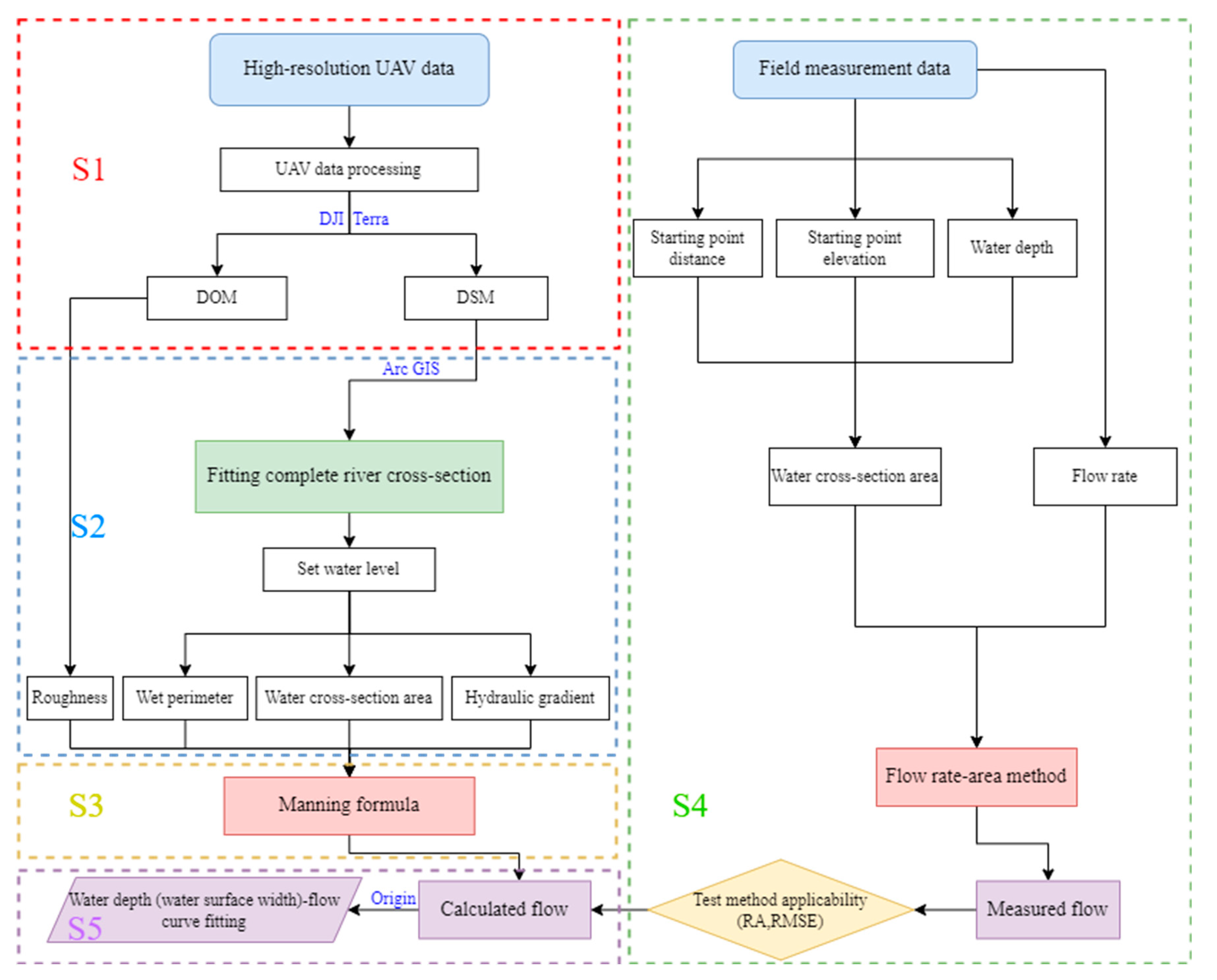
Figure 1. Process of river discharge estimation applied: UAV, unmanned aerial vehicle; DOM, digital orthophoto map; DSM, digital surface model.
Sustainability 14 12792 g001
Figure 2. The geographical location of the Keriya River and the distribution of the selected cross-sections.
Sustainability 14 12792 g002
Figure 3. UAV measuring equipment (a) and UAV flight control software (b).
Sustainability 14 12792 g003
Figure 4. (a) Diagram of the layout of the control points of the image; (b) Field measurement of control points; (c) The control points in UAV aerial survey images.
Sustainability 14 12792 g004
Figure 5. The DOMs and DSMs for each of the six river sections analyzed.
Sustainability 14 12792 g005
Figure 6. Schematic diagram of water depth and flow rate measurement.
Sustainability 14 12792 g006
Figure 7. Photographs of the implemented process for acquiring river cross-sectional data. (a) Measurement cross-section; (b) Researchers field measurements.
Sustainability 14 12792 g007
Figure 8. Flow rate area method flow calculation schematic.
Sustainability 14 12792 g008
Figure 9. G1–G6 river cross-sections (af).
Sustainability 14 12792 g009
Figure 10. Comparison of the fitting effect of different section morphological function models. (a,b) Inclined embankment cross-section; (c,d) Vertical embankment cross-section.
Sustainability 14 12792 g010
Figure 11. Water surface width–flow relationship curve (af);Water depth–flow relationship curve(gl).
Sustainability 14 12792 g011
Figure 12. Typical cross-sectional patterns for the middle and lower reaches of the Keriya River: (a) flat bottom type, (b) protruding bottom type.
Sustainability 14 12792 g012
Figure 13. Braided flow grooves over water in: (a) an ideal state and (b) an actual situation.
Sustainability 14 12792 g013
Table 1. Basic UAV parameters.
UAV ModelPhantom-4-RTK
Camera ModelFC6310R
Image SensorSony Exmor R CMOS
Camera Pixels20 million (5472 × 3648)
Aperturef2.8–f11
Camera focal length8.8 mm
Field of view84°
Maximum line height500 m
Takeoff weight1391 g
Maximum level flight speed50 km·h−1 (positioning mode)
Operating ambient temperature58 km·h−1 (Attitude mode)
Table 2. UAV aerial survey flight control parameters for each measurement area.
ParameterRiver Section
G1G2G3G4G5G6
Flight height (m)100100100100100100
Parallel overlap rate (%)707070707070
Vertical overlap rate (%)808080808080
Survey area (m2)459,898.2453,897.4449,523.8275,247.0190,831.3149,268.8
Ground resolution (cm)2.742.742.742.742.742.74
Table 3. Calculation of the hydraulic gradient in the study river section.
ParameterRiver Cross-Section
G1G2G3G4G5G6
Upstream elevation (m)1201.831219.431244.411261.381275.421297.17
Downstream elevation (m)1201.471219.021243.841261.021275.031296.73
Spacing (m)500500500500500500
Hydraulic gradient0.00070.00080.00110.00070.00080.0009
Table 4. Hydraulic radius calculations of the water crossing sections.
ParameterRiver Cross-Section
G1G2G3G4G5G6
G2-1G2-2G3-1G3-2
Cross-sectional area (m2)10.751.177.688.31.8214.6210.2615.38
Wet perimeter (m)65.028.0630.0440.0210.0353.0337.0260.08
Hydraulic radius (m)0.170.150.260.210.180.280.280.26
Table 5. River flow calculation results.
ParameterRiver Cross-Section
G1G2G3G4G5G6
G2-1G2-2G3-1G3-2
Hydraulic gradient0.00070.00080.00080.00110.00110.00070.00080.0009
Hydraulic radius (m)0.170.150.260.210.180.280.280.26
Roughness0.030.030.030.030.030.030.030.03
Flow (m3·s−1)2.863.223.865.464.116.20
Table 6. Measured data of the underwater cross-section.
Sub-
section
G1G2G3G4G5G6
Area Ai (m2)Flow Rate
v i ¯ (m·s−1)
Flow
Qi (m3·s−1)
Area Ai (m2)Flow Rate
v i ¯ (m·s−1)
Flow
Qi (m3·s−1)
Area Ai (m2)Flow Rate v i ¯ (m·s−1)Flow Qi (m3·s−1)Area Ai (m2)Flow Rate v i ¯ (m·s−1)Flow Qi (m3·s−1)Area Ai (m2)Flow Rate v i ¯ (m·s−1)Flow Qi (m3·s−1)Area Ai (m2)Flow Rate v i ¯ (m·s−1)Flow Qi (m3·s−1)
10.200.050.010.150.050.010.400.100.041.180.200.240.850.200.171.030.100.10
20.600.150.090.230.150.030.730.150.111.980.400.791.980.450.891.430.150.21
30.900.350.320.160.200.030.580.100.061.600.400.642.050.501.030.650.100.07
41.300.500.650.170.200.030.680.200.141.600.450.721.880.551.030.450.100.05
51.450.400.580.160.200.031.230.500.611.700.500.851.450.500.730.580.150.09
60.800.200.160.140.200.031.750.701.231.700.450.771.030.300.311.250.400.50
70.350.100.040.130.200.031.950.601.171.480.400.590.780.150.121.880.651.22
80.400.100.040.060.100.011.000.250.251.250.400.500.100.050.012.130.751.59
90.450.100.050.150.100.020.200.200.041.100.400.44 2.630.751.97
100.830.200.170.540.250.140.400.300.120.850.300.26 2.000.651.30
111.450.400.580.810.350.280.400.200.080.200.100.02 0.800.350.28
121.450.400.580.800.350.280.470.200.09 0.150.150.02
130.580.150.090.620.250.150.370.150.06 0.140.150.02
14 0.590.350.200.100.050.01 0.180.150.03
15 0.920.550.50 0.180.150.03
16 1.320.600.79 0.050.050.00
17 1.350.550.74
18 0.600.250.15
Measured total flow QS (m3·s−1)3.343.453.995.804.277.47
Table 7. Calculated flow accuracy analysis.
ParameterRiver Cross-Section
G1G2G3G4G5G6
Measured flow (m3·s−1)3.343.453.995.804.277.47
Calculated flow (m3·s−1)2.863.223.865.464.116.20
Absolute error (m3·s−1)0.480.230.130.340.161.27
Relative error RA (%)14.376.673.265.863.7517.00
Table 8. Fitting equations of water surface width–flow relationship curves and coefficients of determination (R2).
Cross-SectionFitting EquationR2
G1y = −80.56 × exp (x/−4.15) − 77.25 × exp (x/−4.19) − 40.10 × exp (x/−271.80) + 177.130.991
G2y = −27.47 × exp (x/−3.37) − 51.65 × exp (x/−3.37) − 54.1 × exp (x/−3.37) + 134.280.992
G3y = 51.21 × x0.29 − 18.230.982
G4y = −38.21 × exp (x/−0.25) − 24.15 × exp (x/−15.61) − 23.69 × exp (x/−15.61) + 87.670.988
G5y = 208.16 × x0.02 − 180.580.962
G6y = −42.13 × exp (x/−4.85) − 40.86 × exp (x/−4.85) − 39.72 × exp (x/−4.85) + 125.240.988
Table 9. Fitting equations of water depth–flow relationship curves and coefficients of determination (R2).
Cross-SectionFitting EquationR2
G1y = 0.05 + 0.18 × x0.390.998
G2y = −0.08 + 0.44 × x0.240.997
G3y = −0.04 + 0.29 × x0.340.999
G4y = 0.07 + 0.18 × x0.470.999
G5y = 0.08 + 0.15 × x0.550.999
G6y = 0.07 + 0.24 × x0.370.996
Publisher’s Note: MDPI stays neutral with regard to jurisdictional claims in published maps and institutional affiliations.