Article

Investigation on Dynamic Responses’ Characteristics and Fatigue Damage Assessment for Floating Offshore Wind Turbine Structures

1
Shandong Provincial Key Lab of Ocean Engineering, Ocean University of China, Qingdao 266100, China
2
Envision Energy Co., Ltd., Shanghai 200001, China
3
POWERCHINA Fujian Electric Power Engineering Co., Ltd., Fuzhou 350003, China
*
Author to whom correspondence should be addressed.
Sustainability 2022, 14(19), 12444; https://doi.org/10.3390/su141912444
Submission received: 16 July 2022 / Revised: 22 September 2022 / Accepted: 24 September 2022 / Published: 29 September 2022
(This article belongs to the Topic Wind, Wave and Tidal Energy Technologies in China)

Abstract

:
Dynamic response analysis and fatigue damage assessment of floating offshore wind turbine (FOWT) structures are carried out in this paper with a focus on the statistical characteristics of the dynamic responses under wind–wave excitation. A proper spectral fatigue damage model is proposed to obtain better fatigue damage estimation. The OC3 floating spar (Hywind) with a 5 MW baseline wind turbine developed by the American National Renewable Energy Laboratory (NREL) is applied as the target model, and the fully coupled dynamic responses of the model are calculated in the time domain. The non-Gaussian nature is revealed based on the study of the statistical properties of the dynamic response of key components (the tower base and fairlead of the mooring line). Dirlik distribution is proved to be the best probability distribution function (PDF) that can fit the statistical distribution feature of the dynamic responses among several PDFs. The corresponding spectral fatigue damage models are applied to estimate fatigue damage of the tower base and mooring line following the proposed fatigue assessment procedure in the frequency domain, of which the results are compared with results from the time-domain analysis method. The results indicate that for non-Gaussian feature dynamic responses as FOWTs, the spectral fatigue damage model based on the Dirlik distribution can provide more accurate assessments of fatigue damage.

1. Introduction

Compared to onshore wind turbines, offshore wind turbines (OWTs) have a much broader application space. However, the complex marine environments bring huge challenges to the safety and reliability of OWTs [1,2]. Significant development of OWT technologies has been witnessed over the decades. Various supporting structures have been developed to fit different environments, including fixed and floating types [3]. Due to the good performance in deep waters where the wind energy resources are more abundant, floating OWTs are considered a fast-evolving technology with tremendous prospect [4].
For the years of services, the assessment of fatigue damage is necessary and required by industry standards in the design phase. The spectral method is one of the most popular techniques to evaluate the fatigue damage with the advantages of less computation time and storage space [5]. For the procedures of spectral fatigue damage assessment as well as reliability evaluation, the structural response amplitude/range distribution is one of the most important key factors.
Nowadays, the experience gained from the oil and gas industry is used for the fatigue damage assessment of the offshore wind structures as well [6]. In the traditional procedure, the linear structural responses due to waves are usually assumed to be Gaussian and narrow-banded [7]. The stress amplitudes in each short-term stationary sea state can be described with the Rayleigh distribution and the long-term statistics by the Weibull distribution [8]. However, for OWTs, wind load will influence the dynamic response more significantly than the traditional marine structures used in the oil and gas industry. The bandwidth of the aerodynamic response is wide [6], leading to the question if the traditional Gaussian distribution can describe the statistics characteristics of responses properly.
To estimate the fatigue damage induced by the non-Gaussian response process accurately, two main approaches have been proposed [8]. One is to introduce bandwidth correction factors to modify the narrow-band approximation [9,10,11,12,13,14]. Benasciutti and Tovo [14] discussed and compared these methods and concluded the Dirlik method is the best one. The other approach is to focus on the power density function (PDF) of the response amplitude. A lot of work has been carried out on the statistical model of marine structures [15,16,17].
For the OWT structure, Yeter et al. [6] evaluated the fatigue damage of a fixed jacket OWT in several spectral fatigue damage models including the Rayleigh, Wirsching–Light, Tunna, α0.75, Tovo and Benasciutti, Zhao–Baker, Rice and Dirlik models. The analysis demonstrates that the wide-band solutions are far superior to the narrow-band ones in terms of fatigue damage estimation. Dong et al. [18] used a two-parameter Weibull function and generalized Gamma function to fit the long-term statistical distribution of hot-spot stress ranges in operational conditions of the multi-planar tubular joints of a jacket-type offshore wind turbine. The difference between the two functions is little.
The above research is mainly on the fixed OWT. For deep-sea floating structures, the dynamic responses act quite different from the fixed structure, because they are typically subjected to bimodal loads, consisting of a wave frequency (WF) component due to the first-order wave forces and a low frequency (LF) component induced by the second-order wave forces [15]. Li et al. [8] investigated the statistical characteristics of mooring lines of a semisubmersible platform and validated the non-normality of the line tension response. A modified Gamma distribution is presented to give a more accurate assessment of the fatigue damage.
The objective of this paper is to investigate the statistical characteristics of dynamic responses of offshore wind turbine structures with focus on the non-Gaussian nature of floating structures and propose a proper spectral fatigue damage model to obtain better fatigue damage estimation. To achieve this goal, the OC3 Spar FOWT presented by NREL is selected and the OC3 monopile OWT is also included as a comparison. A joint probabilistic model of mean wind speed, significant wave height and spectral peak period in the Northern North Sea is used to define environmental conditions (wind/sea states). Dynamic responses are calculated under 97 wind–wave combined sea states in the time domain. The non-Gaussian nature is proved by comparing the kurtosis and skewness coefficients of the mooring line tensions with Gaussian distribution. The appropriate distribution functions are presented for the tower base stress and mooring line tension, respectively. Based on the distributions, the fatigue damages of the tower base and mooring line are estimated with the spectral method and compared with the results from the traditional distributions, in which the fatigue damage assessed with the time-domain analysis method is considered as the benchmark.
The remainder of this paper is organized as follows. The theoretical probability distributions presented to describe the statistical characteristics of the structural responses are introduced in Section 2. The commonly used fatigue assessment methods in ocean engineering are explained in Section 3. The model parameters are listed in Section 4. In Section 5, the environmental conditions are determined, the dynamic responses are calculated and the statistical characteristics of axial stresses from the tower base are investigated. In order to propose an appropriate distribution model to describe the short- and long-term statistical distribution of tension amplitude, the non-Gaussian characteristics of the mooring line tension are further analyzed. Moreover, the fatigue damages of the OWT tower base and mooring lines are estimated by spectral analysis method in the frequency domain. Finally, the main conclusions of this study are drawn in Section 6.

2. Distribution of Structural Dynamic Response Amplitudes

For most marine structures, the dynamic responses under the exciting loads are random variables, which can be described by a probability density function (PDF) in statistics. There have been some theoretical probability distributions presented to describe the statistical characteristics of the structural responses.

2.1. Gaussian Distribution

Gaussian distribution, which is also known as normal distribution, has two characteristic parameters including the mean value and the standard deviation, and the PDF of the Gaussian distribution is
f ( x ) = 1 2 π σ e x p ( ( x μ ) 2 2 σ 2 )
where μ is the mean value of x, and σ is the standard deviation of x. In the ocean engineering field, the wave elevation and the linear structural responses can be well fitted by the Gaussian distribution.

2.2. Rayleigh Distribution

The linear responses of offshore structures and ships subjected to wave loads are always considered as Gaussian processes. The short-term response amplitudes of ocean structures follow the Rayleigh distribution. The PDF can be expressed as
f ( x ) = x σ 2 e x p ( x 2 2 σ 2 ) , x 0
where σ is the standard deviation of x.

2.3. Weibull Distribution

The Weibull distribution has been shown to fit many stress spectra for marine structures subjected to wave loads in the offshore oil and gas industry [18]. The PDF of two-parameter Weibull distribution can be written as
f ( x ) = k λ ( x λ ) k 1 e x p ( ( x λ ) k ) , x 0
where k and λ are the shape and scale parameters, respectively. And the mean value μ and standard deviation σ are the functions of k and λ, as
{ μ = λ Γ ( 1 + 1 k ) σ 2 = λ 2 [ Γ ( 1 + 2 k ) Γ 2 ( 1 + 1 k ) ]
where Γ in the Gamma function and can be expressed as Equation (5) at the value t,
Γ ( t ) = 0 + x t 1 e x p ( x ) d x
and k and λ can be calculated through the Equation (4) by the numerical method.

2.4. Dirlik Distribution

Dirlik [11] proposed an empirical method to explore the response spectral density functions of different shapes through the Monte Carlo method and finally gave an empirical formula, known as the Dirlik distribution, which is formed by the superposition of an exponential distribution and two Rayleigh distributions, as follows:
f D K ( x ) = 1 σ y [ B 1 Q 1 e x Q 1 + B 2 Q 2 2 e x 2 2 Q 2 2 + B 3 x e x 2 2 ]
x is expressed as the response amplitude S after standardized processing,
x = S σ y , σ y = 2 m 0
The calculation of each parameter in the formula is as follows:
{ B 1 = 2 ( x m α 2 2 ) 1 + α 2 2 B 2 = 1 α 2 B 1 + B 1 2 1 Q 2 B 3 = 1 B 1 B 2 x m = m 1 m 0 ( m 2 m 4 ) 1 2 , α 2 = m 2 ( m 0 m 4 ) 1 2 Q 1 = 1.25 ( α 2 B 3 B 2 Q 2 ) B 1 Q 2 = α 2 x m B 1 2 1 α 2 B 1 + B 1 2  

2.5. Tovo and Benasciutti Method

Tovo and Benasciutti [14] proposed a response amplitude distribution function based on narrow-band simulation. The distribution function is modeled on the Rayleigh distribution, and its related parameters are calculated by spectral moments and irregular coefficients. The distribution expression is shown as follows:
f T B ( x ) = b γ x m 0 e x p ( x 2 2 m 0 ) + ( 1 b ) x γ 2 m 0 e x p ( x 2 2 γ 2 m 0 )
where γ and b in the function and can be expressed as
γ = m 2 m 2 m 4
b = 1 ( α 2 1 ) 2 ( α 1 α 2 ) a
a = [ 1.112 ( 1 + α 1 α 2 α 1 α 2 ) e x p ( 2.11 α 2 ) + α 1 α 2 ]

3. Fatigue Damage Assessment Method

At present, the commonly used fatigue assessment methods in ocean engineering mainly include the spectral analysis method and time-domain analysis method.

3.1. Spectral Analysis Method

The fatigue damage analysis methods in the frequency domain are mainly based on the PDF of the response amplitude. Combined with the S-N/T-N curve [19,20], and the Palmgren–Miner linear fatigue damage accumulation theory [21], the annual fatigue damage of the structure under the ith load case can be given as
D i = n i N i = 0 365 × 24 × 3600 p i f 0 i f i ( S ) A / S m d S
where S is the stress range; f 0 i   is the average zero-up crossing frequency of the response in Hertz during the ith sea state;   p i   is the probability of occurrence of the ith sea state; f i is the PDF of the structural response range under the ith sea state; and A and m are the empirical coefficient of the S-N/T-N curve.
The total annual fatigue damage is calculated by the superposition of annual fatigue damages under all the load cases, as:
D = i D i
From Equations (13) and (14), one can conclude that the response amplitude distribution is vital to the fatigue damage assessment in the frequency domain. Based on the probability distributions presented in the last section, some spectral fatigue damage calculation models are introduced in the following.
  • Narrow-band solution (Rayleigh)
Substituting Equation (2), the formula for calculating the fatigue based on Rayleigh narrow-band distribution per unit time is given as:
D N B = f 0 i A 1 ( 2 2 σ y ) m Γ ( 1 + m 2 )
2.
Dirlik method
Substituting Equation (6), the expression of fatigue damage by the Dirlik method is given as
D D K = f p A 1 ( 2 σ y ) m · [ D 1 Q 1 m Γ ( 1 + m ) + ( 2 ) m Γ ( 1 + m 2 ) ( D 2 | Q 2 | m + D 3 ) ]
where f p represents the peak rate of the response spectrum.
3.
Tovo–Benasciutti method
Rychlik [22] believes that for a response process conforming to the Gaussian distribution, the calculated value of fatigue damage can be represented by an interval as
D R C D D N B
where DRC is the fatigue damage given by the range-mean counting method [23] as
D R C = f p A 1 ( 2 2 σ y α 2 ) m Γ ( 1 + m 2 )
and DNB is the fatigue damage with respect to the narrow-band solution as in Equation (15).
Based on the Tovo and Benasciutti distribution PDF in Equation (9), Benasciutt [14] gave the empirical formula of fatigue damage estimation based on two fatigue algorithms of D R C   and D N B , as
D T B = b D N B + ( 1 b ) D R C
in which the weight parameter, b, is calculated as in Equations (11) and (12).
The subsequent frequency domain fatigue spectrum analysis methods will use the three methods above for calculation.

3.2. Time-Domain Analysis Method

The time-domain analysis method is considered as the most accurate fatigue assessment method. The structural responses are expressed as stress or tension time histories, and fatigue damage occurs as a result of cycles. The rainflow-counting method [24] is used to complete the statistics of the response amplitude and the corresponding number of cycles [25].
Then, the fatigue damage of the structure is calculated based on the S-N/T-N curve and the PM linear fatigue damage accumulation theory by DNV [26]. The fatigue damage amount under the ith load case is calculated as [20]:
D i = T ( 365 × 24 × 3600 p i T i n i N i )
T i represents the simulation duration of the ith load case.
p i represents the probability of occurrence of the ith load case in annual wind–wave scatter diagram.
n i represents the number of cycles associated with the response range under the ith load case.
N i represents the number of cycles to failure at the response range, which is calculated from S-N/T-N curve.
By accumulating fatigue damage of all load cases in the scatter diagram, the total annual fatigue damage can be obtained, as
D = i D i = i T ( 365 × 24 × 3600 p i T i n i N i )

4. Wind Turbine Models

4.1. NREL 5 MW Wind Turbine

The wind turbine applied in this study is the NREL 5 MW offshore baseline wind turbine model. Its properties are drawn and extrapolated from operating machines and conceptual studies. Its general properties are described in Table 1.

4.2. OC3 Monopile Fixed OWT

At present, due to its simplicity in installation and cost saving, monopile is the most widely used foundation for offshore wind turbines in shallow water depth. A commonly used monopile is a hollow steel member with an outer diameter of 3–6 m and a length of 22–40 m, which is inserted into the seabed soil under seawater, shown in Figure 1. The Offshore Code Comparison Collaboration (OC3) has proposed a monopile with the NREL offshore 5 MW wind turbine for code-to-code verification exercises [28]. In this paper, the monopile fixed OWT was applied and the related properties are list in Table 2.

4.3. OC3-Hywind Spar FOWT

In this paper, the “OC3-Hywind” system presented by NREL is taken as the target FOWT, shown in Figure 2. The system consists of the NREL 5 MW reference turbine and a spar-buoy concept supporting structure developed by Statoil of Norway [29]. The foundation is a spar buoy with a long and slender cylinder shape. It has the advantages of low center of gravity and good stability as the spar platform used in the oil and gas industry. The detailed properties of the floating structure are shown in Table 3. The base of the tower is located at an elevation of 10 m above the still water level (SWL) to the top of the floating platform. The top of the tower is coincident with the yaw bearing and is located at an elevation of 87.6 m above the SWL.
There are three mooring lines for the mooring system, shown in Figure 3. One of the lines (Line 3) is directed along the positive X-axis (in the XZ plane). The two remaining lines (Lines 1 and 2) are distributed uniformly around the platform, such that each line, fairlead and anchor is 120° apart when looking from above. Properties of mooring lines are listed in Table 4.

5. Numerical Study

5.1. Environmental Condition

In this paper, a joint probabilistic model of wind and waves presented by Johannessen et al. [29] is applied to define the sea states. The joint PDF of 1 h mean wind speed at 10 m U w , significant wave height H s and spectral peak period T p can be calculated as:
f U w , H s , T p ( u , h , t ) = f U w ( u ) f H s | U w ( h | u ) f T p | H s , U w ( t | h , u )
The marginal distribution of U w can be described by the two-parameter Weibull distribution. The two-parameter Weibull distribution was suggested as the conditional distribution of H s for given wind speed U w . The conditional distribution of T p for given U w and H s is described by a log-normal distribution.
Considering the fatigue damage in operational conditions as well as the occurrence probability of wind speed, wave height and spectral peak period, respectively, the ranges of environmental parameters are limited as: the range of 1 h mean wind speed U w is 2–22 m/s with an increment of 2 m/s; significant wave height H s is 1–7 m with an increment of 2 m; the range of spectral peak period T p is 4–16 s with an increment of 2 s. Eliminating those states with very small occurrence probability, all 97 different combinations of   U w , H s and T p are considered. The cumulative probability of occurrence is 95.63%, calculated by using the joint probability density distribution given in Equation (22).
The JONSWAP spectrum and IEC Kaimai model are adopted for simulating the random sea state. It is assumed that the wind and waves are always from the same direction, and only one direction is considered for all sea states to avoid a five-dimensional scatter diagram [18]. In this paper, the excitation direction is set to be along the x-axis.
For simplicity’s sake, all the chosen sea states are labeled from 1 to 97 with the increase of the mean wind speed, significant wave height and spectral peak period. For example, U w = 2 m/s, H s = 1 m, T p = 6 s is No. 1, U w = 2 m/s, H s = 1 m, T p = 8 s is No. 2 and U w = 22 m/s, H s = 7 m, T p = 12 s is No. 97.
Based on the wave mechanic, it is generally believed that the undulation of waves is a random process of stationarity and ergodicity with Gaussian distribution characteristics. Figure 4 displays a statistical result of wave elevation under load case (LC) No. 64 where U w is 12 m/s, H s is 5 m and T p is 8 s. As an input state, the convergent statistical result for LC No. 64 shows that the simulated wave elevation follows a Gaussian distribution very well, which suggests that the simulation duration is adequate and that the time step employed is small enough to capture variation details.

5.2. Coupled Dynamic Response in Time Domain

The dynamic response analysis of the OC3 FOWT is performed in the time domain using the computer-aided-engineering (CAE) tool developed by NREL named FAST (Fatigue, Aerodynamics, Structures, and Turbulence). It can solve the coupled aero-hydro-servo-elastic problems with a series of modules [31]. The simulation time length is set to be 7200 s with a 0.1 s time step. Five different random seeds of wind and waves are applied for each state to obtain a proper prediction of the dynamic responses. Shown in Figure 5 and Figure 6 are the obtained tower base force and mooring line tension histories under LC No. 64.

5.3. Analysis of Axial Stress at the Tower Base for Both Fixed and Floating OWT

The tower base of OWT has been considered as a critical part that is prone to becoming damaged from balancing the vibration excitation from the wind turbine and waves [32]. The statistical characteristics of axial stresses from the tower base are investigated in this section. In addition, for obtaining a better understanding of the influences from the different types of structures on the tower base response characteristics, the results from the OC3 fixed monopile are also provided as a comparison.

5.3.1. Axial Stress Calculation

The tower base section is simplified as a thin-walled cylinder structure (Figure 7) without the considerations of welding effects and the connection components between the tower and platform [8]. Therefore, a stress concentration factor of 1.0 is applied in this paper [33] (the hot stress is proportional to this value). The fatigue damage should be calculated for both axial and shear stress components, but the fatigue damage that resulted from shear stress is significantly lower than that from axial stress [34]. Thus, the axial stress is the only component to be considered in the fatigue damage calculation.
For the calculation of axial stress, the cross-section of the tower base is divided into 12 points along the circumferential direction, with an interval of 30° between each action point. The axial stress for a location (r,   θ ) can be written as
σ = N z A + M y I y · r · c o s   θ M x I x · r · s i n   θ
where N z is the axial force, M x and M y are the force in the roll and pitch directions, respectively, I x and I y are the moment of inertia to the corresponding coordinate axis, A is the cross-sectional area, r is effective radius and θ is the angle between the calculated point and point 1.

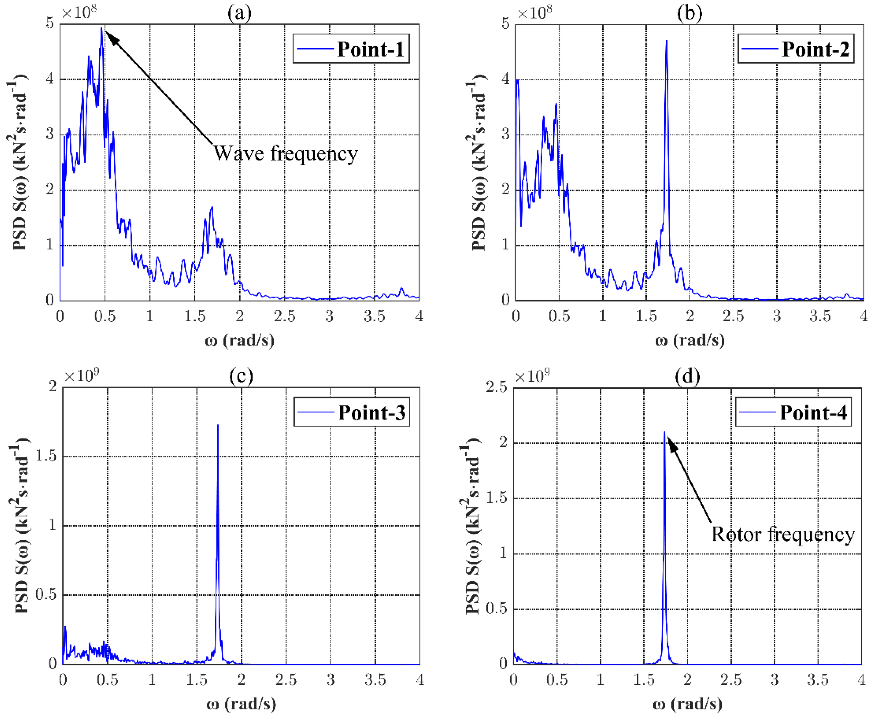
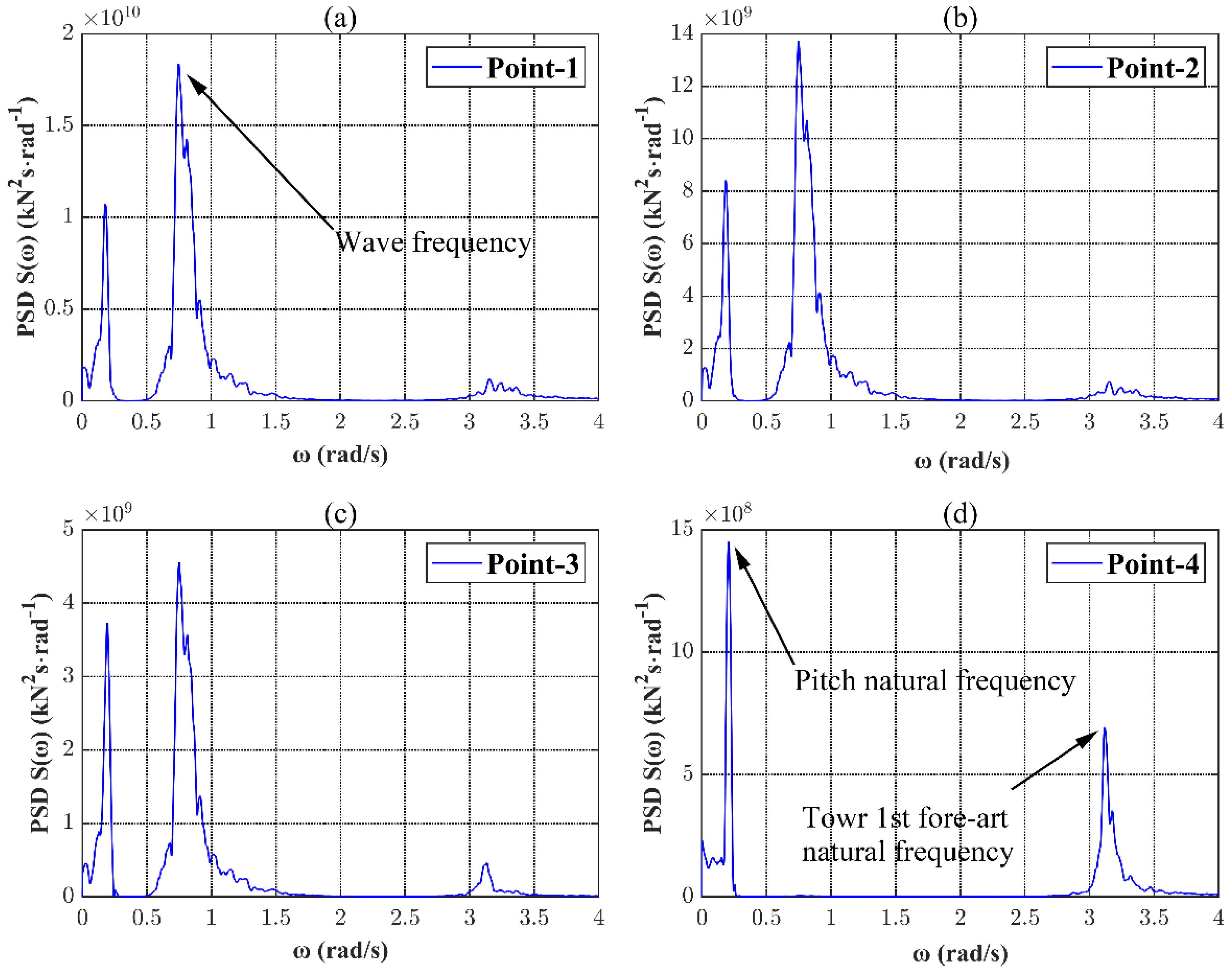
5.3.2. Spectrum Analysis of the Stress at Tower Base

To explore the characteristics of the response spectrum of the stress at the tower base, the response spectra are obtained by performing Fourier transform. According to the response spectrum, the main excitation frequency that causes the stress response and its corresponding spectrum value can be identified. The power spectral density (PSD) spectrum of the stresses at tower base under the LC 64 environment is taken as an example shown in Figure 8.
From Figure 8, the main excitation frequencies of the stress responses are caused by wave loads and the rotation of the wind turbine. Under the condition that the wind speed is greater than the rated wind speed of the wind turbine, the nacelle rotor reaches the maximum speed. The 1P–3P frequency caused by the rotation of the wind turbine is ω = 1.269 rad/s~3.807 rad/s. For point 1, which coincides with the direction of the wind and wave load, the frequency regions caused by the rotation of the wind turbine blade (rotor frequency) and the wave load (wave frequency) can be found clearly. And for point 4, the direction of which is perpendicular to the direction of the wind and waves, the dominated exciting frequency is from the wind turbine. It can be seen from points 1–4 as the angle between the action point and the incident wave direction increases, the dominating exciting frequencies are switching from wave loads to wind turbine loads, and the energy is becoming more concentrated on the wind turbine 1P exciting frequency while the influences of wave loads are becoming smaller.
Figure 9 shows the power spectral density (PSD) spectrum of the tower base stresses of the FOWT. There are three main excitation frequency ranges, which are pitch natural frequency, wave frequency and the first fore-art natural frequency. It can be seen from the response spectrum of point 1 that when the wind and wave load is collinear with the point of action, the pitch motion of the floater and wave frequency are the main excitation frequencies. While at point 4, the response from wave frequency is rather small and the level can be ignored. The trend of the switch of dominated excited frequency is the same as the previous fixed OWT case.
From the response spectrum of the fixed structure and the floating structure, it is obvious that the fixed structure is more sensitive to the excitation frequency of the wind turbine rotor, while for the floating structure, the low frequency effect caused by the natural frequency of the structure is more obvious.

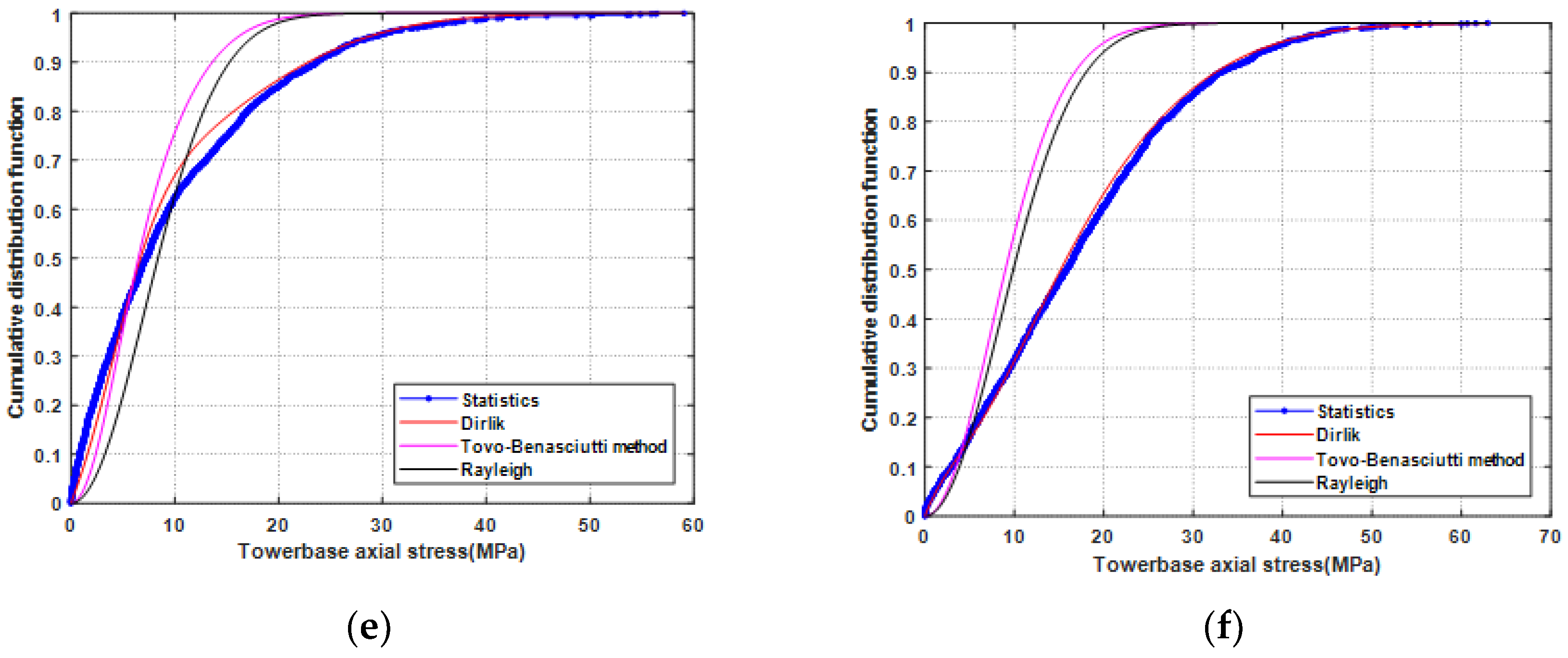
5.3.3. Distribution of Axial Stress Amplitudes of Tower Base

The cumulative distribution functions (CDFs) of axial stress amplitudes of the tower base under each load case are calculated from the time series with the rainflow-counting method. Due to the Gaussian nature of the wave load, it is usually assumed that the short-term distribution of the structural response amplitude under the wave load follows the Rayleigh distribution. To explore the stress amplitude distribution of the tower bases of the fixed and floating structure under short-term sea conditions, the Dirlik distribution and Tovo–Benasciutti distribution are introduced as a comparison. The following six load cases are selected for illustration, as listed in Table 5. The selected load case covers the sea states of small wind and waves (LC 1), moderate wind and waves (LC 33), approximate rated wind speed (LC 45), large wind and small waves (LC 59), large wind and moderate waves (LC 64) and large wind and waves (LC 94).
Figure 10 and Figure 11 show the distribution of the stress amplitude at point 1 of the fixed and floating OWT tower base under the short-term sea conditions.
For the fixed monopile OWT, the distribution of stress response amplitude can follow Rayleigh distribution well under a small sea state (LC 1). As the sea state becomes severe, the distributions no longer follow the Rayleigh distribution, and the Dirlik and Tovo–Benasciutti distributions have better performance. For the load case with harsh wind and waves (LC 94), the Dirlik distribution shows a perfect match with the statistical result.
However, for FOWT, no matter whether the load conditions are mild or severe, the fits between the Rayleigh distribution and the statistical values are not well. The Dirlik distribution has a better match compared to other distributions, especially for the larger stress range. The results indicate FOWT exhibits stronger structural nonlinearity compared to the fixed OWT.

5.4. Analysis of Mooring Line Tension for FOWT

As the nonlinear nature of FOWT has been revealed in last section, this section attempts to go further to analyze the non-Gaussian characteristics of the mooring line tension via kurtosis and skewness tests and consider the effects of both wave frequency component and low frequency component. In the following discussion, the statistical analysis is also conducted to present the proper distribution models to describe the short- and long-term statistical distributions of the tension amplitude.

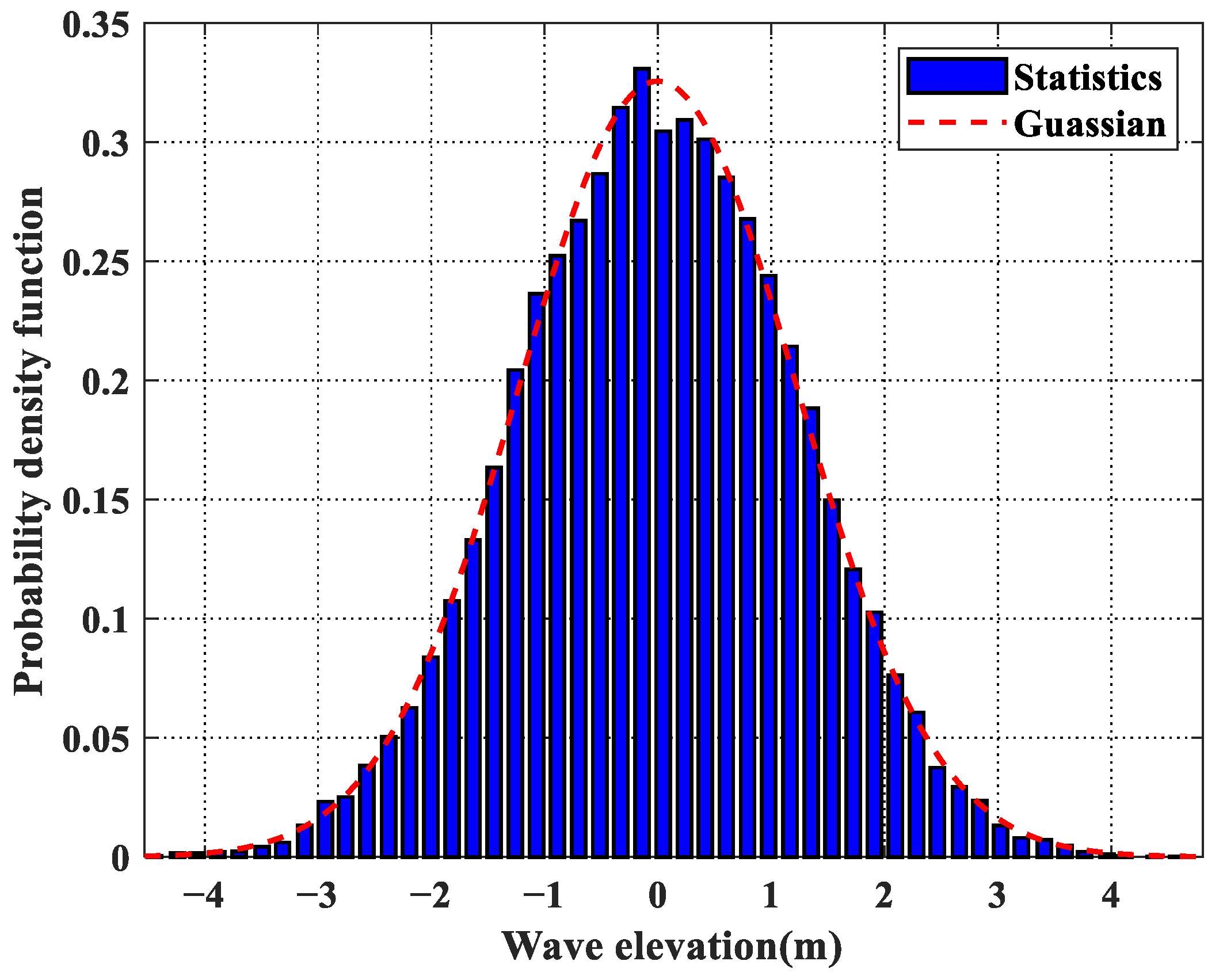
5.4.1. Non-Gaussian Characteristics of Mooring Line Tension Responses

As shown in Figure 12, the spectral analysis method is conducted on the mooring line tension time series to acquire the PSD value and separate total tension into wave frequency (WF) and low frequency (LF) components under LC 64. It can be found that the mooring line time series is obviously comprised of WF and LF components, which are theoretically excited by the first- and second-order wave force, respectively. As the PSD value of mooring line tension shows, on one hand, the response concentrates on two main frequency zones, which are the low frequency zone (about 0.01 Hz) and the wave frequency zone (about from 0.08 Hz to 0.15 Hz); on another hand, the PSD value of the LF component is much larger than the WF component. This indicates that the LF component plays a more dominant role in the response compared with the WF component, and its effect should be considered importantly.
To study the non-Gaussian characteristics of the mooring line tension, kurtosis and skewness coefficients, which are the quantification of the non-Gaussian characteristics of a random process, are calculated from the tension time series. Concretely, the kurtosis is a measure of the “peakedness” of the probability distribution, which corresponds to fourth moments of the density function. The skewness characterizes the asymmetry of the surface distribution and is associated with the third moments of the PDF. The kurtosis and skewness coefficients of any univariate Gaussian distribution are 3 and 0, respectively. It is common to compare the kurtosis and skewness coefficients of a distribution to these values. Excess or insufficient kurtosis coefficient describes the steep or slight peaks, respectively. Negative or positive skewness coefficient indicates that the distribution has a longer tail on the left or right, respectively.
The kurtosis and skewness coefficients of mooring line #3 tension under all 97 load cases are calculated and shown in Figure 13. Also plotted in Figure 13 are the coefficients of kurtosis (value 3) and skewness (value zero) of a Gaussian distribution for comparison. From Figure 13, one can see that the kurtosis and skewness coefficients of mooring line tension fluctuate (more or less) with the load cases, which means wind and wave parameters can affect the Gaussian nature of the mooring line tension significantly. A large proportion of results, especially for the skewness coefficient, evidently show large differences to those of the Gaussian distribution. This indicates that the mooring line tension of FOWT obviously shows the non-Gaussian characteristics.
To study the effects of different frequency components on the non-Gaussian characteristics, the performance of mooring line tension can be discussed for its separate LF and WF components in all load cases. To capture the statistical features of dynamic WF and LF tension, the kurtosis and skewness coefficients of these two parts under all wind and wave load cases are calculated and analyzed, respectively. As shown in Figure 14a,b, the result of the WF mooring line tension can fit the Gaussian hypothesis both in kurtosis and skewness coefficients under most of the load cases. However, the LF mooring line tension displays almost the opposite results, which shows that the LF component seldom supports the Gaussian hypothesis. From Figure 14c,d, one can see that the coefficient of the skewness is positive for almost all the load cases, meaning that the LF mooring line tension distribution has a longer tail on the right compared with the Gaussian distribution. By comparing the statistical kurtosis and skewness coefficients of the total mooring line tension and its separate LF and WF components with Gaussian distribution, it is demonstrated that there are large differences between the mooring line tension statistics and the fitted Gaussian distribution for most load cases, and the LF component especially plays the dominant role in it. The non-Gaussian characteristics of the mooring line tension response are significant and cannot be ignored.
To determine the effect of such non-Gaussian characteristics, several typical load cases (LC6, U w = 2 m/s, H s = 3 m and T p = 8 s; LC 18, U w = 4 m/s, H s = 3 m and T p = 12 s; LC 56, U w = 10 m/s, H s = 5 m and T p = 12 s) are selected for the further detailed illustration. The statistical distribution of mooring line tension and filtered LF and WF components are shown in Figure 15. Also plotted in Figure 15 are the fitted Gaussian distributions for comparison purposes. The differences between the mooring line tension statistics and the fitted Gaussian distribution can be seen clearly from these figures. For LC6 as a benign sea state, the fitting with Gaussian distribution, especially the WF part, is good. As for LC 18, on the one hand, comparing with Gaussian distribution, the peak area is steeper, which means that the mooring line tension response is focused on the “peakedness”; on the other hand, the curve of the mooring line tension is basically symmetrical with slight skewness, which is close to zero. On the contrary, load case LC 56 shows slight kurtosis and obvious skewness whose skewness coefficient is significantly larger than zero, but the kurtosis coefficient is close to three.
From the results of the filtered LF and WF components shown in Figure 15, it is indicated that the Gaussian distribution can fit the WF component of the mooring line tension better than the LF component, which indicated that the LF mooring line tension has stronger non-Gaussian characteristics because of the greater effect of the mooring line nonlinearity on the LF response. Since the Gaussian distribution cannot describe the distribution of the LF component of the mooring line tension properly, the total mooring line tension cannot be satisfactorily fitted by the Gaussian distribution. Like the distribution characteristics of LF component, there are obvious discrepancies between the statistical data and the estimated Gaussian distribution. The above study demonstrates that the mooring line tension response under the most load cases, especially the condition with three-larger kurtosis and positive skewness, is typically a non-Gaussian random process, so that the non-Gaussian characteristics of mooring line tension cannot be ignored.

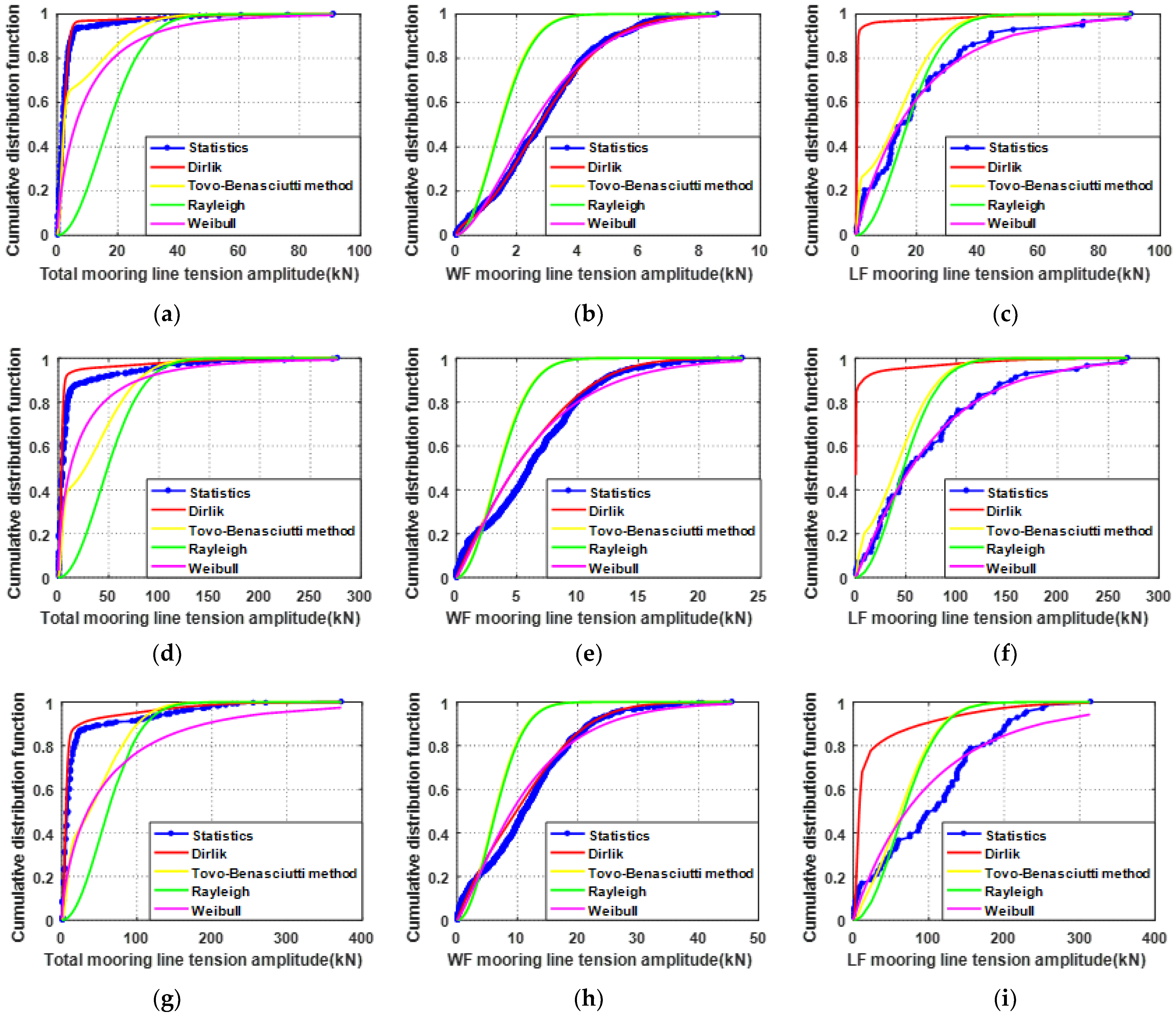
5.4.2. Distribution of Mooring Line Tension Amplitudes

The investigation on the distribution of mooring line tension amplitudes will be focused on in this part. Mooring line tension amplitudes and their cycles are counted from the time series with the rainflow-counting method. A comparison between the cumulative distribution function of counting cycle amplitudes and the theoretical probability distributions presented in Section 2, including the classical narrow-band Rayleigh function, Weibull distribution, Tovo–Benasciutti method and Dirlik’s approximate formula, is shown in the following study to obtain the proper probability distributions of the mooring line tension amplitudes.
Three typical load cases are chosen to illustrate the distributions of total mooring line tension and filter LF and WF components. The first load case is No. 6 with U w = 2 m/s, H s = 3 m and T p = 8 s, in which the kurtosis and skewness coefficients of the mooring line tension are both close to the values of the Gaussian distribution. The second load case is No. 18 with U w = 4 m/s, H s = 3 m and T p = 12 s, in which the kurtosis coefficient is significantly larger than three and the skewness coefficient is close to zero. Load case No. 56 ( U w = 10 m/s, H s = 5 m and T p = 12 s) is selected as the third load case under which the skewness coefficient is significantly larger than zero, but the kurtosis coefficient is close to three.
As illustrated in Figure 16, the difference between mooring line tension statistics data and the fitted distributions can be observed. Among the Rayleigh, Weibull, Tovo–Benasciutti and Dirlik distributions, the Dirlik distribution is the best one to describe the total mooring line tension for all the chosen load cases. As described in the last section, load case No. 6 follows the Gaussian distribution better than those of load cases No. 18 and No. 56, whose kurtosis or skewness is quite different with the Gaussian characteristic. However, Dirlik distribution can make an appropriate description to all the chosen load cases. To check the effect of different components of mooring line tension, the filter LF and WF components’ statistics data are also shown in Figure 16. It is determined that Dirlik distribution is still able to show a good performance of the WF amplitude, mainly because the WF component is more like the broadband Gaussian process. On the contrary, the LF amplitude shows completely different results compared with total mooring line tension and WF tension amplitude. As shown in Figure 16c,f,i, Rayleigh distribution, Tovo–Benasciutti method and Weibull distribution are suitable for describing the LF tension amplitude distribution with respect to the condition of a small tension amplitude range. However, when non-Gaussian is enhanced, the Weibull distribution is found to always be conservative for large cycles, whereas the Rayleigh distribution and Tovo–Benasciutti method have larger probability in a large mooring line tension zone, which can overestimate the structure fatigue damage.
To survey the effect of the wind load and wave load including significant wave heights and peak-spectral period on the selection of the distribution model exactly and clearly, the statistical tension amplitude is calculated under different wave parameters with constant wind speed and different wind speed with constant wave parameters. Three load cases, whose wind speed is unchanged at 12 m/s and the wave parameters increase steadily, are presented in Figure 17. It can be observed that as wave heights change from 3 m to 7 m and the peak-spectral period changes from 8 s to 12 s, the statistical mooring line tension amplitude can make a better performance to the Dirlik distribution. Similarly, as shown in Figure 18, the load cases with constant wave parameters with H s = 3 m and T p = 8 s obtain better fitness to Dirlik distribution when its wind speed increased from 10 m/s to 14 m/s.
To verify the applicability of the Dirlik distribution to the tension response amplitude under short-term sea conditions, the Kolmogorov–Smirnov (K-S) test method was used to test the distribution fit of all 97 sea conditions. It quantifies a distance between the empirical distribution of the sample and the reference distribution by the significance level. If the distance is smaller than the significance level, the fitting is good; otherwise, the fitting is bad. The significance level is determined by the confidence interval and the sample size 7. Here, the number of samples was 300, and the confidence interval was 95%. Then, the significance level can be calculated as
D = 1.36 n = 1.36 300 = 0.0785
From Figure 19, the Dirlik distribution performs as a good fit distribution for most sea states, while the fitting effect of the Rayleigh distribution is not ideal, and the Tovo–Benasciutti distribution is somewhere in between. Therefore, for short-term sea conditions, the mooring line tension response amplitude of offshore wind power structures can be fitted with the Dirlik distribution, and the Rayleigh distribution in the traditional assumption will no longer be applicable.

5.5. Fatigue Damage Assessments of OWT Structures

From the results of the last section, under the coupling action of wind, wave loads and the significant nonlinear factors of the OWT system itself, the probability distribution of the responses no longer satisfies the assumption of the Rayleigh distribution. In this section, the fatigue damages of the OWT tower base and mooring lines are estimated by spectral analysis method in the frequency domain. Various spectral fatigue damage calculation models (as listed in Section 3.1) are applied based on the probability distributions presented in the last section. All 97 load cases as well as the corresponding occurrence probabilities in Section 5.1 are taken as the annual wind–wave scatter diagram. The results are compared with those from the time-domain method, which is taken as reference to testify the validation of the proposed response probability distributions.

5.5.1. Fatigue Damage Assessment of the Tower Base

The fatigue damage of the tower base of both fixed and floating OWTs is first calculated by the time-domain method. To clearly describe the fatigue damage difference between the two structures, the annual fatigue damage of point 1 (Figure 7) of the fixed OWT is taken as the reference, and the other results are normalized as shown in Table 6. It can be observed that under the same scatter diagram, the tower base of FOWT has larger fatigue damage than the fixed OWT.
Then, the annual fatigue damages of the tower base of the two structures are estimated by the frequency domain spectrum method based on the stress amplitude distributions mentioned in Section 5.3. The comparison results are listed in Table 7 and Table 8, where the fatigue damage of point 1 calculated by the time-domain analysis method is still taken as the reference.
From the results, the differences between various spectral fatigue models in fatigue damage estimation can be observed. The fatigue damage result from Dirlik distribution is the closest to the time-domain analysis method, followed by the Tovo–Benasciutti method, while the traditional Rayleigh distribution has a large difference. From Table 7, for the fixed OWT, the differences between the fatigue damage results from the Rayleigh distribution and the time-domain method are significant for points 1 and 2, as the response spectra of points 1 and 2 are obvious broadband (as in Section 5.3.2). Fatigue damage calculations based on the Rayleigh distribution will be significantly overestimated, resulting in a lower prediction value of fatigue life. At points 3 and 4, the fatigue damage results from the frequency domain method are all close to the time-domain method, which indirectly proves the accuracy of the Rayleigh distribution for the evaluation of narrowband response spectra.
For the FOWT, as shown in Table 8, the Rayleigh distribution overestimates the fatigue damage to a large extent compared with the results from the time-domain method. This is because the response spectrum of the floating structure shows obvious broadband characteristics. The results also give the conclusion that the Rayleigh distribution is too conservative for fatigue damage assessment of FOWTs. The fatigue damage calculated by Dirlik distribution is closer to the time-domain method. This method underestimates the fatigue damage to a certain extent, but except for point 3, which is slightly greater than 10%, the errors of the remaining points are within 5%, which belongs to the acceptable error range in practice.

5.5.2. Fatigue Damage Assessment of Mooring System

The fatigue damages of all the three mooring lines of the FOWT are first estimated by the time-domain method. Mooring line #1 with the smallest fatigue damage is taken as reference, and the fatigue damages of the remaining two mooring lines are normalized as shown in Figure 20.
From Figure 20, mooring lines #2 and #3 in the heading direction, the fatigue damage is significantly greater than that of mooring line #1. Then, the Rayleigh, Dirlik and Tovo–Benasciutti spectral fatigue damage calculation models obtained in Section 5.4.2 are applied to calculate the fatigue damage of the mooring system by the frequency domain spectrum method. The comparison results are listed in Table 9, where fatigue damage of mooring line #1 calculated by the time-domain analysis method is normalized as one.
Similar to the results of the tower base in the last subsection, as the mooring line tension series is proved to be a non-Gaussian process, when the Rayleigh distribution is used for fatigue damage calculation, it will produce obvious fatigue damage overestimation, with nearly 15%. The results obtained by using the Dirlik distribution are closer to the time-domain method, although it underestimates the fatigue damage, indicating that the spectral fatigue model is basically accurate in predicting the fatigue damage of the mooring line.

6. Conclusions

Because of the unique excitation loads, the FOWTs have different dynamic behaviors with other floating marine structures in the oil and gas industry. The statistical characteristics of dynamic responses and fatigue damage assessment methods of FOWTs are investigated in this paper. The OC3-Hywind spar FOWT with “5 MW baseline” wind turbine presented by the NREL are applied as target structures. The coupled dynamic responses of critical members (tower base and fairlead) of the FOWT under annual wind–wave sea states are calculated. Through the statistics analysis of the time-domain responses, the non-Gaussian nature is verified, and the proper distribution models are presented to describe the short-term and long-term distribution of stress and tension amplitudes. Based on the different fatigue spectral models, the traditional frequency domain spectrum analysis fatigue calculation method is improved, and the results of the time-domain fatigue calculation method are compared. The main conclusions are as follows:
  • For the tower base of both fixed and floating OWTs, the dominated excitation frequencies of the stress responses are different. For the fixed structure, it is more sensitive to the excitation generated by the rotation of the wind turbine, while for the floating structure, the structure response is more sensitive to the low-frequency wave excitation.
  • The non-Gaussianity of the mooring line tension response is obvious under most of the sea states. Research results show that the non-Gaussian nature of mooring line tension is mainly caused by low-frequency components, while wave-frequency components have little effect on it.
  • The traditional Rayleigh distribution cannot fit both of the stress amplitude of the tower base and tension amplitude of mooring line distribution. Among several candidates of distribution models, the Dirlik distribution has a better performance to describe the statistical characteristics of the FOWT dynamic response.
  • For the fatigue damage assessment, the traditional spectrum analysis method based on the Rayleigh distribution will no longer be applicable to offshore wind turbine structures. This method will overestimate the fatigue damage of the structure to a great extent, while the spectral fatigue damage model with Dirlik distribution shows the close results with those from the time-domain method, indicating that the distribution is suitable for the fatigue damage assessments of FOWTs.

Author Contributions

Conceptualization, M.Z. and J.D.; methodology, J.D. and Y.W.; validation, M.Z., Y.S. and Y.W.; data curation, Z.Z., Y.S. and Y.W.; writing—original draft preparation, M.Z., Y.S. and Y.W.; writing—review and editing, M.Z., Z.Z., K.X. and J.D.; project administration, M.Z.; funding acquisition, M.Z. All authors have read and agreed to the published version of the manuscript.

Funding

This research was funded by the National Natural Science Foundation of China (grant numbers 51879247 and 52171281).

Institutional Review Board Statement

Not applicable.

Informed Consent Statement

Not applicable.

Data Availability Statement

Not applicable.

Conflicts of Interest

The authors declare no conflict of interest.

References

  1. Jonkman, J. Dynamics Modeling and Loads Analysis of an Offshore Floating wind Turbine; NREL/TP-500-41959; National Renewable Energy Laboratory: Golden, CO, USA, 2007.
  2. Ren, Y.; Venugopal, V.; Shi, W. Dynamic analysis of a multi-column TLP floating offshore wind turbine with tendon failure scenarios. Ocean Eng. 2022, 245, 110472. [Google Scholar] [CrossRef]
  3. Zhang, Y.; Shi, W.; Li, D.; Li, X.; Duan, Y.; Verma, A.S. A novel framework for modeling floating offshore wind turbines based on the vector form intrinsic finite element (VFIFE) method. Ocean Eng. 2022, 262, 112221. [Google Scholar] [CrossRef]
  4. Feng, K.; Ji, J.C.; Ni, Q. A novel adaptive bandwidth selection method for Vold–Kalman filtering and its application in wind turbine planetary gearbox diagnostics. Struct. Health Monit. 2022, 475–501. [Google Scholar] [CrossRef]
  5. Ariduru, S. Fatigue Life Calculation by Rainflow Cycle Counting Method. Master’s Thesis, Middle East Technical University, Ankara, Turkey, 2004. [Google Scholar]
  6. Yeter, B.; Garbatov, Y.; Guedes Soares, C. Evaluation of fatigue damage model predictions for fixed offshore wind turbine support structures. Int. J. Fatigue 2016, 87, 71–80. [Google Scholar] [CrossRef]
  7. Gao, Z.; Moan, T. Frequency-domain fatigue analysis of wide-band stationary Gaussian processes using a trimodal spectral formulation. Int. J. Fatigue 2008, 30, 1944–1955. [Google Scholar] [CrossRef]
  8. Li, H.; Du, J.; Wang, S.; Sun, M.; Chang, A. Investigation on the probabilistic distribution of mooring line tension for fatigue damage assessment. Ocean Eng. 2016, 124, 204–214. [Google Scholar] [CrossRef]
  9. Wirsching, P.H.; Light, M.C. Fatigue under wide band random stresses. J. Struct. Div. 1980, 106, 1593–1607. [Google Scholar] [CrossRef]
  10. Rice, S.O. Mathematical analysis of random noise. Bell Syst. Tech. J. 1945, 24, 46–156. [Google Scholar] [CrossRef]
  11. Dirlik, T. Application of Computers in Fatigue Analysis. Ph.D. Thesis, University of Warwick, Coventry, UK, 1985. [Google Scholar]
  12. Oritz, K.; Chen, N.K. Fatigue damage prediction for stationary wide-band stresses. In Proceedings of the 5th International Conference on the Applications of Statistics and Probability in Civil Engineering, Vancouver, BC, Canada, 8–12 June 1987. [Google Scholar]
  13. Kim, B.; Wang, X.Z.; Shin, Y.S. Extreme load and fatigue damage on FPSO in combined waves and swells. In Proceedings of the 10th International Symposium on Practical Design of Ships and Other Floating Structures, Houston, TX, USA, 1–5 October 2007. [Google Scholar]
  14. Benasciutti, D.; Tovo, R. Spectral methods for lifetime prediction under wide-band stationary random processes. Int. J. Fatigu. 2005, 27, 867–877. [Google Scholar] [CrossRef]
  15. Gao, Z.; Moan, T. Fatigue damage induced by nongaussian bimodal wave loading in mooring lines. Appl. Ocean Res. 2007, 29, 45–54. [Google Scholar] [CrossRef]
  16. Jiao, G.; Moan, T. Probabilistic Analysis of Fatigue Due to Gaussian Load Process. Probab. Eng. Mech. 1990, 5, 76–83. [Google Scholar] [CrossRef]
  17. Park, J.-B.; Chang, Y.S. Fatigue damage model comparison with formulated tri-modal spectrum loadings under stationary gaussian random processes. Ocean Eng. 2015, 105, 72–82. [Google Scholar] [CrossRef]
  18. Dong, W.; Moan, T.; Gao, Z. Long-term fatigue analysis of multi-planar tubular joints for jacket-type offshore wind turbine in time domain. Eng. Struct. 2001, 33, 2002–2014. [Google Scholar] [CrossRef]
  19. American Bureau of Shipping. Guide for the Fatigue Assessment of Offshore Structures; American Bureau of Shipping (ABS): Houston, TX, USA, 2003. [Google Scholar]
  20. API Recommended Practice2SK(RP2SK). Recommended Practice for Design and Analysis of Station Keeping Systems for Floating Structures: Exploration and Production Department; American Petroleum Institute: Washington, DC, USA, 2005. [Google Scholar]
  21. Miner, M.A. Cumulative damage in fatigue. J. Appl. Mech. 1945, 12, 159–164. [Google Scholar] [CrossRef]
  22. Rychlik, I. On the ‘narrow-band’ approximation for expected fatigue damage. Int. J. Fatigue 1994, 16, 235. [Google Scholar] [CrossRef]
  23. Tovo, R. Cycle distribution and fatigue damage under broad-band random loading. Int. J. Fatigue 2002, 24, 1137–1147. [Google Scholar] [CrossRef]
  24. Matsuishi, M.; Endo, T. Fatigue of metals subjected to varying stress. Jpn. Soc. Mech. Eng. 1968, 96, 100–103. [Google Scholar]
  25. Du, J.; Chang, A.; Wang, S.; Sun, M.; Wang, J.; Li, H. Multi-mode reliability analysis of mooring system of deep-water floating structures. Ocean Eng. 2019, 192, 106517. [Google Scholar] [CrossRef]
  26. DNV DNV-RP-C203. Fatigue Design of Offshore Steel Structures; DNV: Oslo, Norway, 2010. [Google Scholar]
  27. Jonkman, J.; Butterfield, S.; Musial, W. Definition of a 5-MW Reference Wind Turbine for Offshore System Development; National Renewable Energy Lab: Golden, CO, USA, 2009.
  28. Jonkman, J.; Musial, W. Offshore Code Comparison Collaboration (OC3) for IEA Wind Task 23 Offshore Wind Technology and Deployment; National Renewable Energy Lab: Golden, CO, USA, 2010.
  29. Johannessen, K.; Meling, T.S.; Haver, S. Joint distribution for wind and waves in the northern northsea. Int. J. Offshore Polar Eng. 2002, 12, 1–8. [Google Scholar]
  30. Jonkman, J. Definition of the Floating System for Phase IV of OC3; National Renewable Energy Lab: Golden, CO, USA, 2010.
  31. Jonkman, B.; Jonkman, J. ReadMe File for FAST v8; National Renewable Energy Laboratory: Golden, CO, USA, 2014.
  32. Ciang, C.C.; Lee, J.R.; Bang, H.J. Structural health monitoring for a wind turbine system: A review of damage detection methods. Meas. Sci. Technol. 2008, 19, 310–314. [Google Scholar] [CrossRef]
  33. Kvittem, M.I.; Moan, T. Frequency versus time domain fatigue analysis of a semisubmersible wind turbine tower. J. Offshore Mech. Arct. Eng. 2015, 137, 011901.1–011901.11. [Google Scholar] [CrossRef]
  34. Kvittem, M.I.; Moan, T. Time domain analysis procedures for fatigue assessment of a semi-submersible wind turbine. Mar. Struct. 2015, 40, 38–59. [Google Scholar] [CrossRef] [Green Version]
  35. Li, H.; Hu, Z.; Wang, J.; Meng, X. Short-term fatigue analysis for tower base of a spar-type wind turbine under stochastic wind-wave loads. Int. J. Nav. Archit. Ocean Eng. 2018, 10, 9–20. [Google Scholar] [CrossRef]
Figure 1. OC3 monopile fixed OWT [28].
Sustainability 14 12444 g001
Figure 2. OC3-Hywind spar FOWT [30].
Sustainability 14 12444 g002
Figure 3. Mooring distribution of the floating wind turbine [30].
Sustainability 14 12444 g003
Figure 4. Statistical result of wave elevation under LC No. 64.
Sustainability 14 12444 g004
Figure 5. Time series of tower base force in LC No. 64.
Sustainability 14 12444 g005
Figure 6. Time series of mooring line tension in LC No. 64.
Sustainability 14 12444 g006
Figure 7. Schematic diagram of tower base [35].
Sustainability 14 12444 g007
Figure 8. Stress response spectrum at the tower base of fixed monopile OWT in LC64. (a) Stress response spectrum at point 1; (b) stress response spectrum at point 2; (c) stress response spectrum at point 3; (d) stress response spectrum at point 4.
Sustainability 14 12444 g008
Figure 9. Stress response spectrum at the tower base of FOWT in LC64. (a) Stress response spectrum at point 1; (b) stress response spectrum at point 2; (c) stress response spectrum at point 3; (d) stress response spectrum at point 4.
Sustainability 14 12444 g009
Figure 10. Distribution of stress amplitude at tower base of the fixed monopile OWT. (a) LC 1 ( U w = 2 m/s, H s = 1 m, T p = 6 s); (b) LC 33 ( U w = 6 m/s, H s = 5 m, T p = 12 s); (c) LC 45 ( U w = 8 m/s, H s = 5 m, T p = 12 s); (d) LC 59 ( U w = 12 m/s, H s = 1 m, T p = 6 s); (e) LC 64 ( U w = 12 m/s, H s = 5 m, T p = 8 s); (f) LC 94 ( U w = 18 m/s, H s = 7 m, T p = 14 s).
Sustainability 14 12444 g010aSustainability 14 12444 g010b
Figure 11. Distribution of stress amplitude at tower base of the FOWT. (a) LC 1 ( U w = 2 m/s, H s = 1 m, T p = 6 s); (b) LC 33 ( U w = 6 m/s, H s = 5 m, T p = 12 s); (c) LC 45 ( U w = 8 m/s,   H s = 5 m, T p = 12 s); (d) LC 59 ( U w = 12 m/s, H s = 1 m, T p = 6 s); (e) LC 64 ( U w = 12 m/s, H s = 5 m, T p = 8 s); (f) LC 94 ( U w = 18 m/s, H s = 7 m, T p = 14 s).
Sustainability 14 12444 g011aSustainability 14 12444 g011b
Figure 12. PSD of mooring line tension and filtered WF and LF components under LC 64.
Sustainability 14 12444 g012
Figure 13. Kurtosis and skewness coefficients of mooring line #3 tension under all 97 load cases. (a) Kurtosis; (b) skewness.
Sustainability 14 12444 g013
Figure 14. Kurtosis and skewness coefficients of WF and LF mooring line tension under all 97 load cases. (a) Kurtosis coefficients of WF component; (b) skewness coefficients of WF component; (c) kurtosis coefficients of LF component.; (d) skewness coefficients of LF component.
Sustainability 14 12444 g014
Figure 15. Distribution of mooring line tension and filtered LF and WF components. (a) Total tension ( U w = 2 m/s, H s   = 3 m, T p   = 8 s); (b)WF component ( U w   = 2 m/s, H s   = 3 m, T p   = 8 s); (c) LF component ( U w   = 2 m/s, H s   = 3 m, T p   = 8 s); (d) total tension ( U w   = 4 m/s, H s   = 3 m, T p   = 12 s); (e) WF component ( U w   = 4 m/s, H s   = 3 m, T p   = 12 s); (f) LF component ( U w   = 4 m/s, H s   = 3 m, T p   = 12 s); (g) total tension ( U w   = 10 m/s, H s   = 5 m, = 12 s); (h) WF component ( U w   = 10 m/s, H s   = 5 m, T p   = 12 s); (i) LF component ( U w   = 10 m/s, H s   = 5 m, T p   = 12 s).
Sustainability 14 12444 g015
Figure 16. Cumulative distribution function of mooring line tension and filtered LF and WF components under chosen load cases. (a) Load case No. 6 ( U w = 2 m/s, H s   = 3 m, T p   = 8 s); (b) load case No. 6 ( U w   = 2 m/s, H s   = 3 m, T p   = 8 s); (c) load case No. 6 ( U w   = 2 m/s, H s   = 3 m, T p   = 8 s); (d) load case No. 18 ( U w   = 4 m/s, H s   = 3 m, T p   = 12 s); (e) load case No. 18 ( U w   = 4 m/s, H s   = 3 m, T p   = 12 s); (f) load case No. 18 ( U w   = 4 m/s, H s   = 3 m, T p   = 12 s); (g) load case No. 56 ( U w   = 10 m/s, H s   = 5 m, T p   = 12 s); (h) load case No. 56 ( U w   = 10 m/s, H s   = 5 m, T p   = 12 s); (i) load case No. 56 ( U w   = 10 m/s, H s   = 5 m, T p   = 12 s).
Sustainability 14 12444 g016
Figure 17. Cumulative distribution function of mooring line tension under different wave load case. (a) Load case No. 61 ( U w = 12 m/s, H s   = 3 m, T p   = 8 s); (b) load case No. 64 ( U w   = 12 m/s, H s   = 5 m, T p   = 10 s); (c) load case No. 68 ( U w   = 12 m/s, H s   = 7 m, T p   = 12 s).
Sustainability 14 12444 g017
Figure 18. Cumulative distribution function of mooring line tension under different wind load case. (a) Load case No. 51 ( U w = 10 m/s, H s   = 3 m, T p   = 8 s); (b) load case No. 61 ( U w   = 12 m/s, H s   = 3 m, T p   = 8 s); (c) load case No. 71 ( U w   = 14 m/s, H s   = 3 m, T p   = 8 s).
Sustainability 14 12444 g018
Figure 19. K-S test result of mooring line tension amplitude.
Sustainability 14 12444 g019
Figure 20. Comparison of normalized fatigue damage of mooring line tension.
Sustainability 14 12444 g020
Table 1. NREL 5 MW offshore wind turbine [27].
ParameterValues
Rating5 MW
Rotor Orientation, Configuration
Control
Upwind, 3 Blades
DrivetrainVariable Speed, Collective Pitch
Gearbox
Rotor Diameter, Hub Diameter
Hub Height
126 m, 3 m
90 m
Cut-In, Rated, Cut-Out Wind Speed3 m/s, 11.4 m/s, 25 m/s
Cut-In, Rated Rotor Speed6.9 rpm, 12.1 rpm
Rotor Mass110 t
Nacelle Mass240 t
Tower Mass347.46 t
Table 2. OC3 monopile fixed OWT [28].
ParameterValues
Height of tower87.6 m
Monopile length above water surface10 m
Depth of seawater20 m
Monopile length buried in soil45 m
Diameter of top and bottom of tower3.87 m and 6 m
Thickness of top and bottom of tower0.019 m and 0.027 m
Diameter and thickness of monopile6 m and 0.06 m
Density, young’s modules and shear modules of tower8500 kg/m³, 210 GPa and 80.8 GPa
Density, young’s modules and shear modules of monopile7850 kg/m³, 210 GPa and 80.8 GPa
Table 3. OC3-Hywind floating structure properties [30].
ParameterValues
Depth to platform base below SWL (total draft)120 m
Elevation to platform top (tower base) above SWL10 m
Depth to top of taper below SWL4 m
Depth to bottom of taper below SWL12 m
Platform diameter above taper6.5 m
Platform diameter below taper9.4 m
Platform mass, including ballast7,466,330 kg
CM location below SWL along platform centerline89.9155 m
Water depth320 m
Table 4. OC3-Hywind mooring system properties [30].
ParameterValues
Depth to anchors below SWL (water depth)320 m
Depth to fairleads below SWL70 m
Radius to anchors from platform centerline853.87 m
Radius to fairleads from platform centerline5.2 m
Unstretched mooring line length902.2 m
Mooring line diameter0.09 m
Equivalent mooring line mass density77.7066 kg/m
Equivalent mooring line weight in water698.094 N/m
Equivalent mooring line extensional stiffness384,243,000 N
Table 5. Selected short-term sea conditions.
Load Case No. U w ( m / s ) H s ( m ) T p ( s ) f ( u , h , t )   ( % )
12162.18
3365120.38
4585121.01
5912160.15
6412580.16
94187140.19
Table 6. Normalized annual fatigue damage at the tower based on time-domain calculation.
The PointFixed OWTFOWT
Point 1111.4945
Point 20.59975.3973
Point 30.15740.3777
Point 40.08920.1249
Table 7. Normalized annual fatigue damage at the tower base of fixed OWT.
PointTime DomainRayleighDirlikTovo–Benasciutti
Point 111.34920.92360.9098
Point 20.59970.79740.59270.5800
Point 30.15740.16410.15590.1537
Point 40.08920.09030.08900.0881
Table 8. Normalized annual fatigue damage at the tower base of FOWT.
PointTime DomainRayleighDirlikTovo–Benasciutti
Point 111.42940.98810.9584
Point 20.44440.59750.42680.4136
Point 30.03320.04150.02950.0285
Point 40.01050.01520.01010.0099
Table 9. Normalized annual fatigue damage of the mooring system of FOWT.
LineTime DomainRayleighDirlikTovo–Benasciutti
Line #111.17900.98150.9454
Line #21.72121.97721.63311.5887
Line #31.91442.23351.78691.7289
Publisher’s Note: MDPI stays neutral with regard to jurisdictional claims in published maps and institutional affiliations.

