Assessing the Drivers of Carbon Intensity Change in China: A Dynamic Spatial–Temporal Production-Theoretical Decomposition Analysis Approach

Abstract

As carbon intensity (CI) can better reflect the coordinated relationship between carbon emissions and economic growth, the related research has gradually increased in recent years. To better explore the influence of production technology and spatial variations on CI disparities in China, this paper constructs a dynamic spatial–temporal production-theoretical decomposition analysis (DST-PDA) model to explore the dynamic spatial disparities and temporal variations of driving factors on CI in different regions. Moreover, this paper further investigates the impact of production-related factors, such as carbon emission technology’s change with regard to carbon intensity, and explores the benchmarking catch-up effect and the effort on reducing CI by setting benchmarks and dynamic comparative analysis, which could provide guidance for some underperforming regions. The main results are as follows: (1) The overall trends of CI increased from 2007–2019, and the northwest region had the largest growth rate. (2) Energy intensity was the dominant driver to reduce CI, and technological changes also played a great role in decreasing CI. Conversely, carbon emissions efficiency had negative effects on reducing CI. (3) The spatial variations of the contributions in factors to reduce CI have gradually increased. Resource-dependent development areas have great potential to reduce carbon intensity by improving energy and carbon emission efficiencies. The northwest has great potential to reduce CI by introducing advanced technologies. Some policies are proposed based on the results.

1. Introduction

As the largest carbon dioxide (CO₂) emitter in the world, the growth of CO₂ in China has become a global concern. However, China’s carbon emissions continue to grow. With the rapid development of China’s economy and industrialization, the total CO₂ emissions in China increased by 227.84% during 2000–2020, and the CO₂ emissions in China accounted for 32.48% of the global emissions in 2020 [1]. To better consider the relationship between economic development and carbon emissions, it is reasonable to consider reducing the carbon intensity (CI) of China. At the Copenhagen Climate Conference (2009), China committed to achieving a reduction in CI of 40–45% between 2005 and 2020. Moreover, the Chinese government further proposed an emission reduction target in 2009, which pledged that the CI of China will decline by 60% to 65% by 2030, and strive to achieve “carbon peak” by 2030 and “carbon neutral” by 2060 [2]. Therefore, it is necessary to find the main drivers that could reduce the CI and further help the government formulate targeted emission reduction policies.

The existing studies have explored the effect of the main drivers of CI using decomposition analysis [3,4,5,6] and regression [7,8,9]. Decomposition analysis methods are widely used by many scholars [10,11,12], because they can indirectly or directly decompose the energy-related and carbon-related changes into several factors, such as the energy intensity and economic activity, and further explore the effects of these drivers without external factors. At present, three kinds of decomposition analysis methods have been widely used: structural decomposition analysis (SDA), index decomposition analysis (IDA) and production-theoretical decomposition analysis (PDA).

Generally, the calculation of SDA was proposed by Chang and Lin (1998) [13] and is based on an input–output table. SDA can deeply analyze the structure effect from the consumption and demand dimensions [14,15], but the data are difficult to collect and update. Therefore, the IDA and PDA were proposed, which simplify the complexity of data collection by collecting panel data from provinces or departments in each year. Specifically, IDA can be divided into Divisia and Laspeyres index decomposition modes. The logarithmic mean Divisia index (LMDI) is the most common IDA method because it can be tested by a mutual transfer factor, time mutual transfer, and zero value robustness [16,17]. There have been increasingly more applications in carbon emission decomposition and energy consumption decomposition analysis in recent years [18,19,20].

In addition, the PDA method has been proposed in recent years because it can better measure the effect of technology, which combines the distance function, development envelopment analysis and production technology. This method is of practical significance as it can consider more details in the production process. Specifically, PDA was first applied to the energy field by Zhou and Ang (2008) [21], and this study decomposed carbon emissions in OECD (Organization for Economic Co-operation and Development) countries and explored the effects of seven factors, such as technological progress and the technological efficiency of carbon emissions and energy savings, on carbon emissions. Several researchers have proposed expanded PDA approaches for the province [22], regional [23], cities [24] and sector scale [25]. However, PDA cannot guarantee the accuracy of the structure effect, and the LMDI method can solve this problem effectively. Therefore, some scholars expanded the PDA method into the joint decomposition model, which combines the PDA and LMDI methods to explore the contributions of the drivers of carbon emissions of carbon intensity [26,27,28,29].

From the view of decomposition types, the current decomposition forms can be divided into three types: temporal decomposition, spatial decomposition and temporal–spatial decomposition. Temporal decomposition analysis calculates and compares the decomposition results of factor decomposition in each year, which can address the trend of driving factors over time in a region. Previous research has mainly used this method to analyze the historical trend of carbon emissions or carbon intensity over time, and temporal-IDA, temporal-SDA, and temporal-PDA are all widely used [30,31,32], but they cannot consider regional disparities in depth. Therefore, spatial decomposition analysis was applied in the decomposition field.

The original concept of spatial decomposition was proposed by Ang and Zhang (1999) [33], who considered that regional differences should be considered for comparative analysis, but these differences are not clearly defined in spatial decomposition analysis. Ang et al. (2015) [34] defined and reviewed spatial decomposition in detail and further classified models into three categories: bilateral-region (B-R), radial-region (R-R), and multi-region (M-R) models. Since then, spatial decomposition has been used by many scholars because it can adequately compare the different performances and effects of each region in a certain period in depth [35,36,37]. And the M-R method is more objective and recyclable because of the comparison of the constructed average virtual area, so this method is the most widely used, including spatial-SDA and spatial-IDA [38,39,40]. But the spatial-PDA has few applications [41]. In addition, spatial decomposition is a static decomposition that observes the breakdown over only one year or a few years. To understand the effects of a more comprehensive understanding, Ang et al. (2016) [42] proposed a temporal–spatial decomposition approach from two levels to capture the regional disparities and temporal development trends simultaneously. This method has been gradually applied by some scholars in recent years [43,44,45,46].

In summary, the previous studies have studied the changes of carbon intensity from different aspects, and the characteristics are summarized as follows. First, most research has focused on the temporal decomposition over time within different regions, and only a few studies have focused on spatial decomposition analysis; that is to say, fewer works in the literature have considered spatial differences. Moreover, the application of a joint decomposition model by combining the temporal and spatial differences is even less. However, it is necessary to construct a temporal–spatial decomposition model to consider regional differences and temporal variations. Second, most studies on spatial decomposition selected a specific year as the benchmark, which lacks dynamic comparative analysis. Therefore, it is necessary to construct a spatial–temporal decomposition analysis method that sets up a benchmark area in each year to ensure the relative comparability and prevent external factors from hindering the analysis. Third, most of the spatial decomposition studies used only the SDA and IDA methods, and fewer articles used the spatial-PDA or spatial–temporal-PDA methods, which means that they ignored the regional differences in the production process when measuring the factors impacting CI.

Therefore, this paper introduces a dynamic spatial–temporal production-theoretical decomposition analysis (DST-PDA) model to explore the contributions of driving forces on the change in CI in China. Compared with the existing research, the present work contributes to the literature in three major ways: First, we propose a temporal–spatial model, which can not only capture the characteristics of temporal changes in different years of a specific region, but also can further capture the change in the carbon emissions disparities between different regions. In this context, we can describe the effort of underperforming regions in carbon emissions reduction. Second, this paper combines the temporal–spatial decomposition model with PDA to construct the DST-PDA model, which can better reflect the effect of production technology on the change in CI. Especially, this paper investigates the influence of carbon emission reduction and energy saving technology on the change in CI from a spatial–temporal perspective. Third, differently from the existing literature, which selects reference regions based on a static strategy, i.e., taking a specific region in a specific year or a virtue region as reference region, this paper selects reference regions based on a dynamic strategy, i.e., taking the average performance of all regions each year as the reference region, which can detect detailed dynamic change in the catch-up effect of carbon emissions reduction. The DST-PDA model proposed in this paper can not only decompose the factors related to production technology, such as energy technology efficiency progress and carbon emission efficiency improvement on CI, but also explore the spatiotemporal differences in the impact of these factors on CI, as well as further explore each region in order to reduce CI. More specifically, this model can further explore the efforts made by each region to reduce carbon intensity by exploring the degree of catching up with the benchmark region evaluating the sustainability of such efforts.

The remainder of this paper is organized as follows. Section 2 introduces the dynamic spatial–temporal-PDA model and data sources. Section 3 discusses the decomposition results. Section 4 presents the main conclusions and proposes some suggestions.

2. Methods and Models

2.1. The Production Technology and Distance Function

2.1.1. The Production Technology

Assume that the entire economy consists of I region i (i = 1, …, I). According to Zhou and Ang (2008) [21] and Kim and Kim(2012) [47], the production process can be defined as in the closed set P as Equation (1):

$$P^t=\left\{\left(E^t,K^t,L^t,Y^t,C^t\right)|\left(E^t,K^t,L^t\right)can produce\left(Y^t,C^t\right)\right\}$$

(1)

In Equation (1), energy consumption I, capital (K) and labor (L) are defined as inputs, and gross domestic product (GDP, Y) and carbon emissioI (C) are defined as inputs, desirable outputs, and undesirable outputs. Based on Färe et al. (1989) [48] and Chung et al. (1997) [49], the desirable and undesirable outputs in the closed set P have two characteristics: weak disposability and null-jointness.

According to these characteristics, the environmental production technology P^t in period t can be calculated by using the nonparametric frontier approach in the development envelopment analysis (DEA) programming technique and assuming constant returns to scale (CRS), and it can be defined as Equation (2):

$$P^t=\left\{(E^t,K^t,L^t,Y^t,C^t)|\begin{array}{l}{\displaystyle \sum _{i=1}^I{z}_i{E}_i^t\le E^t},\\ {\displaystyle \sum _{i=1}^I{z}_i{K}_i^t\le K^t},\\ {\displaystyle \sum _{i=1}^I{z}_i{L}_i^t\le L^t},\\ {\displaystyle \sum _{i=1}^I{z}_i{Y}_i^t\ge Y^t,}\\ {\displaystyle \sum _{i=1}^I{z}_i{C}_i^t=C^t}, z_i\ge 0, k=1,2,\dots ,K\end{array}\right\}$$

(2)

2.1.2. The Shephard Distance Function and Estimation Models

The technical efficiency of input and output between the production frontier and the particular entity can be evaluated by the Shephard distance functions. The distance functions of energy consumIon (E), Ission (C), and GDP (Y) can be described as Equation (3) and Equation (4):

$$D_C^t(E_{}^t,K_{}^t,L_{}^t,Y_{}^t,C_{}^t)=\sup \left\{\theta |(E_{}^t,K_{}^t,L_{}^t,Y_{}^t,C_{}^t/\theta )\in P^t\right\}$$

(3)

$$D_E^t(E_{}^t,K_{}^t,L_{}^t,Y_{}^t,C_{}^t)=\sup \left\{\delta |(E_{}^t/\delta ,K_{}^t,L_{}^t,Y_{}^t,C_{}^t)\in P^t\right\}$$

(4)

Equation (3) and Equation (4) minimize the proportion of energy and carbon emissions input given the limited technology, capital and labor inputs, and undesirable and desirable outputs. The conditions of $D_E^t(E_{}^t,K_{}^t,L_{}^t,Y_{}^t,C_{}^t)\ge 1$ and $D_C^n(E_i^n,K_i^n,L_i^n,Y_i^n,C_i^n)\ge 1$ are necessary. Moreover, the production technology is efficient only if $D_E^t(E_{}^t,K_{}^t,L_{}^t,Y_{}^t,C_{}^t)$, $D_C^t(E_{}^t,K_{}^t,L_{}^t,Y_{}^t,C_{}^t)=1$.

The efficiency in the distance function and production technology can be estimated by constructing the DEA technique. The Shephard distance function of energy and carbon inputs and output can be further calculated into the PDA model as Equation (5) and Equation (6).

$$\begin{array}{c}{\left[D_C^t(E_{}^t,K_{}^t,L_{}^t,Y_{}^t,C_{}^t)\right]}^{-1}=\min \theta \\ s.t.\{\begin{array}{l}{\displaystyle \sum _{i=1}^I{z}_i^{}{E}_i^t\le E_i^t}\\ {\displaystyle \sum _{i=1}^I{z}_i^{}{K}_i^t\le K_i^t}\\ {\displaystyle \sum _{i=1}^I{z}_i^{}{L}_i^t\le L_i^t}\\ {\displaystyle \sum _{i=1}^I{z}_i^{}{Y}_i^t\ge Y_i^t}\\ {\displaystyle \sum _{i=1}^I{z}_i^{}{C}_i^t={\theta }_{}{C}_i^t}\\ z_i^{}\ge 0, i=1,2,\dots ,I\end{array}\end{array}$$

(5)

$$\begin{array}{c}{\left[D_E^t(E_{}^t,K_{}^t,L_{}^t,Y_{}^t,C_{}^t)\right]}^{-1}=\min \delta \\ s.t.\{\begin{array}{l}{\displaystyle \sum _{i=1}^I{z}_i^{}{E}_i^t=\delta E_i^t}\\ {\displaystyle \sum _{i=1}^I{z}_i^{}{K}_i^t\le K_i^t}\\ {\displaystyle \sum _{i=1}^I{z}_i^{}{L}_i^t\le L_i^t}\\ {\displaystyle \sum _{i=1}^I{z}_i^{}{Y}_i^t\ge Y_i^t}\\ {\displaystyle \sum _{i=1}^I{z}_i^{}{C}_i^t\le C_i^t}\\ z_i^{}\ge 0, i=1,2,\dots ,I\end{array}\end{array}$$

(6)

where z_i is the weight coefficient, and $E_i^t$, Kit, $L_i^t$, $Y_i^t$, $C_i^t$ are the energy consumption, capital, labor, gross domestic product, and carbon emissions of region i (i = 1, 2, …, I) in period t, $t\in \left\{0,T\right\}$.

2.2. The Spatial–Temporal Decomposition Model

Based on the Kaya identity, the carbon intensity of China can be decomposed as Equation (7):

$$C{I}_i^t=\frac{C_{ij}^t}{Y_{ij}^t}={\displaystyle \sum _i\frac{C_{ij}^t}{E_{ij}^t}\times \frac{E_{ij}^t}{E_i^t}\times \frac{E_{ij}^t}{Y_{ij}^t}},t\in \left\{0,T\right\}$$

(7)

where i represents the different regions and j represents the different types of energy. $C_{ij}^t$ represents the total amount of CO₂ emissions in period t; $E_i^t$ and $E_{ij}^t$ individually represent the energy consumption of region i and the total in period t; $Y_i^t$ and $Y_{ij}^t$ individually denote the gross domestic product of region i and the total in period t, $t\in \left\{0,T\right\}$.

To consider the influence of technical factors in the production process on carbon intensity, this paper introduces the Shephard distance function to construct the PDA decomposition model. The CI can be further decomposed as Equation (8):

$$\begin{array}{ll}C{I}_j^t& =\frac{C_{ij}^t}{Y_{ij}^t}\\ & ={\displaystyle \sum _i\frac{C_{ij}^t/{[D_C^t(E_{}^t,K_{}^t,L_{}^t,Y_{}^t,C_{}^t)D_C^t(E_{}^{t+1},K_{}^{t+1},L_{}^{t+1},Y_{}^{t+1},C_{}^{t+1})]}^{1/2}}{E_{ij}^t}}\times \frac{E_{ij}^t/{[D_E^t(E_{}^t,K_{}^t,L_{}^t,Y_{}^t,C_{}^t)D_E^t(E_{}^{t+1},K_{}^{t+1},L_{}^{t+1},Y_{}^{t+1},C_{}^{t+1})]}^{1/2}}{Y_{ij}^t}\\ & \times D_E^t(E_{}^t,K_{}^t,L_{}^t,Y_{}^t,C_{}^t)\times {\left[\frac{D_E^t(E_{}^{t+1},K_{}^{t+1},L_{}^{t+1},Y_{}^{t+1},C_{}^{t+1})}{D_E^t(E_{}^t,K_{}^t,L_{}^t,Y_{}^t,C_{}^t)}\right]}^{1/2}\times D_C^t(E_{}^t,K_{}^t,L_{}^t,Y_{}^t,C_{}^t)\times {\left[\frac{D_C^t(E_{}^{t+1},K_{}^{t+1},L_{}^{t+1},Y_{}^{t+1},C_{}^{t+1})}{D_C^t(E_{}^t,K_{}^t,L_{}^t,Y_{}^t,C_{}^t)}\right]}^{1/2}\\ & =PCE{F}_{}^t\times PE{I}_{}^t\times E{F}_{}^t\times ETHC{H}_{}^t\times C{F}_{}^t\times CTHC{H}_{}^t\end{array}$$

(8)

The right side of Equation (8) has the following meaning: The first component represents the potential carbon emission factor ($PCE{F}_i^t$), and the second component can be interpreted as potential energy consumption intensity ($PE{I}_i^t$). The other component is related to production technology, in which the third and the fourth components indicate the energy efficiency ($E{F}_i^t$) and the technological change in energy consumption ($ETHC{H}_i^t$), and the fifth and last components are the carbon emission efficiency ($C{F}_i^t$) and the technological change in carbon emissions ($CTHC{H}_i^t$), respectively.

To compare and identify the regional disparities in CI, a spatial decomposition model is proposed. The spatial decomposition can eliminate the influence of regional development differences, thereby putting all regions in a relatively comparable state, and the emission reduction effect and potential can be observed in different regions. The static spatial decomposition of a region in a certain period can be constructed as shown in Equation (9). In this model, the benchmark region that represents the average level of all comparative regions and each pair can be compared to the hypothetical region. In Equation (9), the differences in CI between region n (Rⁿ) and the national average (R*) in t period ($t\in \left\{0,T\right\}$) can be decomposed into the 6 drivers.

$$\begin{array}{ll}{S}_{C{I}_{Rn}}^t& =\frac{C{I}_{Rn}^t}{C{I}_{R*}^t}\\ & =S_{PCE{F}_{Rn}}^t\times S_{PE{I}_{Rn}}^t\times S_{E{F}_{Rn}}^t\times S_{ETHC{H}_{Rn}}^t\times S_{C{F}_{Rn}}^t\times S_{CTHC{H}_{Rn}}^t,t\in \left\{0,T\right\}\end{array}$$

(9)

Equation (9) shows the spatial decomposition of CI in the Rn region: the value of $S_{C{I}_{Rn}}^t$ greater than 1 indicates that the CI of the region Rn is much higher than the reference region R* (the national average), and the CI of the region Rn needs to be further improved.

According to the LMDI model, the driving forces of the CI can be calculated as shown in Equations (10)–(15):

$$S_{PCE{F}_{Rn}}^t=\exp \left({\displaystyle \sum _{j=1}^J\frac{L(C_{iRn}^t,C_{iR*}^t)}{L(C_{Rn}^t,C_{R*}^t)}}\ln \left(\frac{PCE{F}_{Rn}^t}{PCE{F}_{R*}^t}\right)\right)$$

(10)

$$S_{PE{I}_{Rn}}^t=\exp \left({\displaystyle \sum _{j=1}^J\frac{L(C_{iRn}^t,C_{iR*}^t)}{L(C_{Rn}^t,C_{R*}^t)}}\ln \left(\frac{PE{I}_{Rn}^t}{PE{I}_{R*}^t}\right)\right)$$

(11)

$$S_{E{F}_{Rn}}^t=\exp \left({\displaystyle \sum _{j=1}^J\frac{L(C_{iRn}^t,C_{iR*}^t)}{L(C_{Rn}^t,C_{R*}^t)}}\ln \left(\frac{E{F}_{Rn}^t}{E{F}_{R*}^t}\right)\right)$$

(12)

$$S_{ETHC{H}_{Rn}}^t=\exp \left({\displaystyle \sum _{j=1}^J\frac{L(C_{iRn}^t,C_{iR*}^t)}{L(C_{Rn}^t,C_{R*}^t)}}\ln \left(\frac{ETHC{H}_{Rn}^t}{ETHC{H}_{R*}^t}\right)\right)$$

(13)

$$S_{C{F}_{Rn}}^t=\exp \left({\displaystyle \sum _{j=1}^J\frac{L(C_{iRn}^t,C_{iR*}^t)}{L(C_{Rn}^t,C_{R*}^t)}}\ln \left(\frac{C{F}_{Rn}^t}{C{F}_{R*}^t}\right)\right)$$

(14)

$$S_{CTHC{H}_{Rn}}^t=\exp \left({\displaystyle \sum _{j=1}^J\frac{L(C_{iRn}^t,C_{iR*}^t)}{L(C_{Rn}^t,C_{R*}^t)}}\ln \left(\frac{CTHC{H}_{Rn}^t}{CTHC{H}_{R*}^t}\right)\right)$$

(15)

where $L(·)$ can be defined as Equation (16):

$$L(a,b)=\{\begin{array}{ll}\frac{a-b}{\ln a-\ln b},\hfill & a\ne b\hfill \\ a or b,\hfill & a=b\hfill \end{array}$$

(16)

The spatial decomposition results of carbon intensity in each period of 0–t is sorted by time, which is dynamic spatial decomposition, and can dynamically display the changes of carbon intensity and the spatial difference of decomposition factors with the time sequence.

To further explore the dynamic changes in this spatial variation over time, this paper constructs a temporal–spatial production-theoretical decomposition analysis model (ST-PDA) that combines the temporal and spatial decomposition models. The ST-PDA decomposition result of the CI from period 0 to period t can be described as follows:

$$\begin{array}{ll}\frac{S_{C{I}_{Rn}}^t}{S_{C{I}_{Rn}}^0}& =\frac{C{I}_{Rn}^t/C{I}_{R*}^t}{C{I}_{Rn}^0/C{I}_{R*}^0}=\frac{C{I}_{Rn}^t}{C{I}_{Rn}^0}/\frac{C{I}_{R*}^t}{C{I}_{R*}^0}\\ & =S{T}_{PCE{F}_{Rn}}^{t,0}\times S{T}_{PE{I}_{Rn}}^{t,0}\times S{T}_{E{F}_{Rn}}^{t,0}\times S{T}_{ETHC{H}_{Rn}}^{t,0}\times S{T}_{C{F}_{Rn}}^{t,0}\times S{T}_{CTHC{H}_{Rn}}^{t,0}\end{array}$$

(17)

Equation (17) shows the spatial–temporal (ST) decomposition of CI in the Rn region. The factors decomposed by temporal–spatial decomposition can represent the catching-up effect and the efforts to reduce the CI of each region Rn to the benchmark region R*. The decomposition and analysis of such factors are rare in other research centers.

In Equation (17), the result could be expressed as the spatial differences between the researched region (Rn) and the reference region (R*). If the value of $S{T}_{C{I}_{Rn}}^{t,0}$ is less than 1, it means that the CI of the Rn region is trying to approach the reference region R*, which means that it has a strong sense to reduce the CI. This paper defines this as the catch-up effect. Similarly, $S{T}_{PE{I}_{Rn}}^{t,0}$, $S{T}_{E{F}_{Rn}}^{t,0}$, $S{T}_{C{F}_{Rn}}^{t,0}$, $S{T}_{ETHC{H}_{Rn}}^{t,0}$, and $S{T}_{CTHC{H}_{Rn}}^{t,0}$ represent the catch-up effect of the Rn region from 0 to t for the baseline region in each factor (including potential energy consumption intensity, the energy efficiency, the carbon emission efficiency, the technological change in energy consumption, and the technological change in carbon emissions). The value of the ST decomposition result can also demonstrate efforts of a region to reduce CI. Specifically, if the value of a factor, such as $S{T}_{C{F}_{Rn}}^{t,0}$, is less than 1, it means that the Rn of the researched area is trying to close the gap in and the carbon emission efficiency between it and the benchmark area; that is to say, the region Rn is trying to reduce carbon intensity by improving the carbon emission efficiency.

In addition, to better explore the persistence of the catch-up effect in various regions, this paper proposes a dynamic spatial–temporal (DST) decomposition model. The DST decomposition model is to divide the spatial–temporal decomposition results according to different stages of the 0–t period, which can dynamically display the changing trend of the spatial–temporal decomposition results over time. It can show the enthusiasm of each region Rn to catch up with the benchmark region R*, or just to reduce carbon intensity at some stage.

The DST-PDA model proposed in this paper can not only decompose the factors related to production technology, such as energy technology efficiency progress and carbon emission efficiency improvement on CI, but also explore the spatial temporal differences in the impact of these factors on CI, as well as further explore each region in order to reduce CI. More specifically, this model can further explore the efforts made by each region to reduce carbon intensity by exploring the degree of catching up with the benchmark region, and evaluate the sustainability of such efforts.

2.3. Data Sources

This paper analyzes the changes in carbon intensity in 30 provinces (excluding Tibet, Hong Kong, and Taiwan) in China from 2007–2019. To conduct the comparative analysis among regions, according to the report ”Strategies and Policies for Coordinated Regional Development” issued by the Development Research Center of The State Council, we divide the 30 provinces into 8 regions considering their different stages of economic and geographical area, i.e., the northern coast, the eastern coast, the southern coast, the middle of the Yellow River, the middle of the Yangtze River, the central, the northeast, the northwest and the southwest (The northern: Beijing, Tianjin, Hebei, Shandong; the eastern coast: Shanghai, Jiangsu and Zhejiang; the southern coast: Fujian, Guangdong, and Hainan; the middle of the Yellow River: Shaanxi, Henan, Inner Mongolia, and Shaanxi; the middle of Yangtze River: Hubei, Hunan, Jiangxi, and Anhui; the northeast: Liaoning, Jilin, and Heilongjiang; the northwest: Gansu, Qinghai, Ningxia, and Xinjiang; the southwest: Guangxi, Chongqing, Sichuan, Guizhou, and Yunnan). The data of energy consumption (E), labor (L), and GDP (Y) are found in the China Energy Statistics Yearbook and National Bureau of Statistics of China. All the economic data are converted into 2007 (benchmark year) constant prices.

Capital should be calculated by the perpetual inventory method (PIM), which can estimate the total value of capital in China from 2007 to 2016 by converting the real value in the benchmark year value. Similarly, the output (Y) should also be converted by the real GDP in the benchmark year. Moreover, the value of carbon emissions (C) can be calculated based on the eight types of energy consumption. Previous literature has mostly calculated carbon emissions based on the IPCC (2006) [50]. Based on the above, this paper calculated the CO₂ emissions in eight types of energy in different sectors, as shown in Equation (18):

$$C={\displaystyle \sum _{j=1}^J{E}_j\times {\delta }_j}$$

(18)

where E_j represents the energy consumption of energy type j, and ${\delta }_i$ is the carbon emission coefficient (Carbon emission coefficients of fuels (unit: t CO₂/t). Coal: 1.9003; coke: 2.8604; crude oil: 3.0202; gasoline: 2.9251; kerosene: 3.0179; diesel oil: 3.0959; fuel oil: 3.175; liquefied petroleum gas: 3.1013; natural gas: 2.1622; the carbon emission coefficient of electricity is different in different regions.) of energy type j.

3. Results and Discussion

3.1. The Change in CI and Main Drivers

Figure 1 reflects the change in CI in 30 provinces of China from 2007 to 2019. In general, the change in CI in China experienced three stages: a slow decline period (2007–2011), a rapid decline period (2011–2015), and a rebound fluctuation period (2015–2019). Figure 2a shows the cumulative change in CI in eight regions from 2007 to 2019, and the result is less than 1 during the observation period, which means the CI decreased constantly in the past 12 years. As shown in Figure 2a, the CI of the eight regions in China decreased from 2007 to 2019, among which the CI of southwest decreased most rapidly, with a 59.13% decrease compared with 2007. Meanwhile, the northwest region, especially in the Ningxia and Xinjiang provinces, exhibited the worst performance in reducing the CI.

Figure 2b reports the influence of each main factor. When the decomposition value is greater than 1, it means that the factor can increase the growth of the CI; when the decomposition value is less than 1, it means that it will promote the decrease in the CI. In this context, CF and EF were the important factors for the increase in CI, which can increase carbon intensity by 4.17% and 7.39%, respectively. Conversely, EI has the largest influence on reducing CI (8.31%), and CTHCH, PCEF, and ETHCH can also inhibit the growth in CI.

3.2. The Dynamic Spatial–Temporal Decomposition Results

3.2.1. The Cumulative Spatial Decomposition Results at the Regional Level

To explore the spatial differences in CI change and main driving factors in different regions, and further explore the changes of spatial differences over time, this paper introduced a dynamic spatial–temporal decomposition (DST-PDA) model.

Firstly, Figure 3 shows the cumulative spatial decomposition results of the eight regions from 2007–2019. When the result is greater than 1, the consumption of the CI in the region is higher than the national average, which is to say that the factor exhibited poor performance in reducing the CI. Similarly, if the value of the result was less than 1, the region exhibited a better performance in reducing the CI in this factor. As shown in Figure 3, there were large spatial disparities in the CI in eight regions. The northwest had the worst performance in CI reduction: the CI of the northwest is higher than the national average of 158.37%. In addition, the CI of northern coast and the middle of the Yellow River were higher than the average level by 113.18% and 3.29%, respectively. They are the key regions that need to continuously reduce CI and optimize the relationship between CI and economic envelopment. Similarly, PCEF, PEI and CF all have large regional disparities. The cumulative spatial decomposition results from 2007 to 2019 show that there are significant differences in the emission effects of PEI and CF factors in the Northwest, the middle of Yellow River and the northeast compared with other regions in China. That is the main reason for the higher CI of these regions than the national average.

3.2.2. The Dynamic Spatial Decomposition over Time at the Regional Level

Figure 4 presents the change trends of the spatial decomposition result over time in eight regions, we also refer to the results of the dynamic spatial changes of the eight regions. If the value of the spatial is greater than 1, it means that it is well above the national average, and if the value decreases over time, it means that that region is trying to narrow the spatial difference. As shown in Figure 4a–c, the values of $S_{CI}^t$ in the northwest, the middle of the Yellow River and the northeast were far greater than 1 and kept increasing from 2007 to 2019, indicating that the CI in these regions was far higher than the national average level in 2007–2019. In addition, they do not have the consciousness to improve the CI, and the gap between the CI and the national average level is still increasing. The growth rate and spatial difference in CI in different regions are still different. Specifically, the $S_{CI}^t$ in the northwest increased fastest, and while the S_CI of the middle of the Yellow River had a large base in 2007, the increase was small. Additionally, the $S_{CI}^t$ in northeast had a M-shaped increase.

The main factors affecting the different regions are different. As shown in Figure 4c, the CI in the northwest is always higher than the national average level during 2007–2019, and the spatial gap between the regional and the national average continued to increase with time, with the most rapid growth during 2010–3013 and 2016–2019. The main reason for this unsatisfactory CI reduction is the poor performance of PEI and EF. As can be seen from Figure 4c, the negative impact of PEI and CF factors on reduction of CI from 2007–2019 also continued to increase rapidly, which was further away from the national average level. However, it is worth mentioning that the value of $S_{CTHCH}^t$ has been declining from 2007 to 2019, and even below 0 after 2012, which indicates that the CTHCH factor is gradually close to the national average level, and gradually overtakes other regions. This represents that the northwest region has been trying to improve its awareness of catching up with advanced emission reduction technologies from 2007–2019, but its emission reduction efficiency has not been well improved. Similar to the situation in the northwest, the reduction degree of CI in the middle of the Yellow River and the northeast is slower than the national average level, mainly due to the poor performance in the PEI and CF factors on reducing CI, which need to be further improved in the future.

As shown in the Figure 4d, the CI, PEI, CF, CTHCH of the southwest were higher than the national average level before 2015, but they continued to improve from 2007 to 2019, narrowing the gap between it and the national optimal emission reduction region. The value of $S_{CI}^t$ was less than 1 after 2014 and the reduction of CI was significantly higher than other regions. We can say that the southwest had a good catch-up effect in reducing CI from 2007 to 2019. It achieved continuous reduction of CI by catching up with the CF, CTHCH, and PEI of other regions. On the one hand, as shown in the Figure 4e, the decline in CI in the middle of the Yangtze River is always greater than the national average level, and the region is still trying to reduce more carbon intensity from 2007 to 2019, mainly due to the good effect of PEI, CF, and CTHCH factors. On the other hand, the CI of the southern coast and eastern coast are far lower than the national average, and has been maintaining a relatively good rate of emission reduction as shown in the Figure 4f,g. It is mainly due to the better carbon emission efficiency and the improvement of advanced carbon emission reduction technologies. However, as shown in the Figure 4h, the decline in CI of Northern coast in 2007–2016 is not large, which only ensures that the CI is basically equal to the national average level. The re-optimization and re-creation of carbon emission efficiency should be improved.

3.2.3. Spatial Decomposition Result at the Provincial Level

Figure 5 reveals the spatial decomposition results in 30 provinces. As shown in Figure 5, the CI of Ningxia, Gansu, Qinghai, Shaanxi, Inner Mongolia, Shaanxi, Guizhou, Hebei, and Liaoning provinces contributed 365.65%, 256.42%, 266.95%, 143.95%, 49.69%, 95.68%, 59.49%, 63.49%, respectively.

Specifically, the high carbon intensity of Ningxia was mainly due to the poor performance of PEI, which was 477.13% lower than the national average. Similarly, Qinghai and Chongqing also had poor performance on PEI, which were 358.17% and 89.00% lower than the national average, respectively. In addition, the performances of CF in Shandong, Hebei, Liaoning and Xinjiang were 251.52%, 221.75%, 140.11%, 111.42%, 87.65%, and 56.86% lower than the national average, respectively. Similarly, the contributions of EF factors in these provinces to the reduction in emissions were also 22.55%, 43.17%, 319.75%, 10.20%, and 125.15% lower than the national average. Therefore, these provinces have great potential to reduce carbon intensity by improving the CF and EF. Moreover, the performances of ETHCH in Shandong, Liaoning, and Xinjiang were not great either.

In addition, Hubei, Zhejiang, and Shanghai still have great potential to reduce the carbon intensity by improving the CF and EF. In other words, the effects of EF in 11 provinces should be improved to reduce the CI, including Hubei, Zhejiang, Jilin, Hunan, Shanghai, and Shaanxi. Chongqing should improve the PCEF and EI factors, and Jiangsu and Beijing still have large potential to improve PCEF to reduce the CI.

3.3. The Dynamic Spatial–Temporal Decomposition Results

3.3.1. Spatial–Temporal Decomposition Results at the Regional Level

Figure 6 shows the spatial–temporal decomposition results for each factor in the eight regions. Spatial–temporal results can reveal the catch-up effect of each region to the average level, and dynamic spatial–temporal decomposition can reflect the degree of change in catch-up effect. When the spatial–temporal decomposition result is greater than 1, it means that it is gradually moving away from the selected benchmark. When the decomposition result is less than 1, it means that it is gradually approaching the benchmark, that is to say, had a catch-up effect.

Figure 7 illustrates the changes in the temporal–spatial decomposition results in the eight regions of China during 2007–2019. As stated in Section 3.2.2, the spatial performances of the carbon intensity in the northwest, northern coast, the middle of the Yellow River were higher than the benchmark region. As shown in Figure 7a, the values of ST(CI) of the northwest and the middle of the Yellow River were always greater than 1 from 2007 to 2019 and did not achieve close to the baseline regional emission reduction. On the contrary, the ST(CI) values of southwest and the middle of the Yangtze River were always less than 0 during 2007–2019, which means that these regions have been striving to achieve optimal emission reduction effects, and this effort is especially obvious in 2012–2013 and 2014–2015. Other regions have made erratic efforts to reduce CI, sometimes outperforming the benchmark region, and sometimes underperforming it.

In addition, Figure 7b–g present the dynamic spatial–temporal variations in the influence of different factors on the CI. As shown in Figure 8, the average values of $S{T}_{PEI}^{t,0}$ and $S{T}_{EF}^{t,0}$ in the southwest and the middle of the Yangtze River were always less than 1 during 2007–2019, indicating that these regions were always pursuing the optimal carbon emission efficiency and energy intensity to promote the reduction of CI during 2007–2019. However, the pursuit of optimal carbon emission efficiency in both regions decreased after 2014. In addition, the $S{T}_{CF}^{t,0}$ of the eastern coast was always less than 1 from 2007–2019, and it is also constantly improving the CF to achieve the effect of reducing CI.

It is worth noting that the ST(CTHCH) values in almost all regions are less than 1 from 2010 to 2012, which means that all regions made efforts to catch up with the advanced carbon emission technologies in other regions, especially during 2011–2013, which is also the period when China proposed to achieve reduced CI.

3.3.2. Spatial–Temporal Decomposition Results at the Provincial Level

Figure 8 reveals that the temporal–spatial results of the CI in Ningxia, Xinjiang, Qinghai, Chongqing, Shaanxi, and Liaoning were greater than 1, which indicates that the poor performance of the CI in these regions continues to deteriorate. Specifically, the values of $S{T}_{CF}^{t,0}$, $S{T}_{EF}^{t,0}$, $S{T}_{PEI}^{t,0}$, $S{T}_{ETHCH}^{t,0}$ and $S{T}_{CTHCH}^{t,0}$ in Ningxia, Xinjiang, Shaanxi and Chongqing provinces were all greater than 1, which indicates that the expansion speed of spatial difference increases each day. On the other hand, for Liaoning Province, CF is the main reason for the spatial differences in its poor CI performance; the value of $S{T}_{CF}^{t,0}$ in Liaoning Province was 1.0657, and the PCEF, EF, and EI were also the reasons for its poor performance.

4. Conclusions and Policy Implications

This paper constructed a dynamic temporal–spatial PDA model to explore the factors influencing the carbon intensity based on panel data from 2007 to 2019 in China. Specifically, this paper deeply discusses the changes in the influence of spatial differences on carbon emission reduction per unit GDP (carbon intensity) by combining spatial analysis and temporal–spatial analysis. The main conclusions are as follows:

(1)

Overall, the CI of China decreased by an average of 3.67% per year during 2007–2019. The CI of the southwest and the middle of the Yangtze River region decreased the fastest, by 4.99% and 4.54% per year during 2007–2019. In addition, the CI of the downward trend can be divided into three periods: slow decline period, rapid decline period, and gentle fluctuation period. Energy intensity (PEI) and technological changes in carbon emissions (CTHCH) were the determinant factors for reducing carbon emissions, while the efficiency of carbon emissions (CF) was the main factor for increasing carbon intensity.

(2)

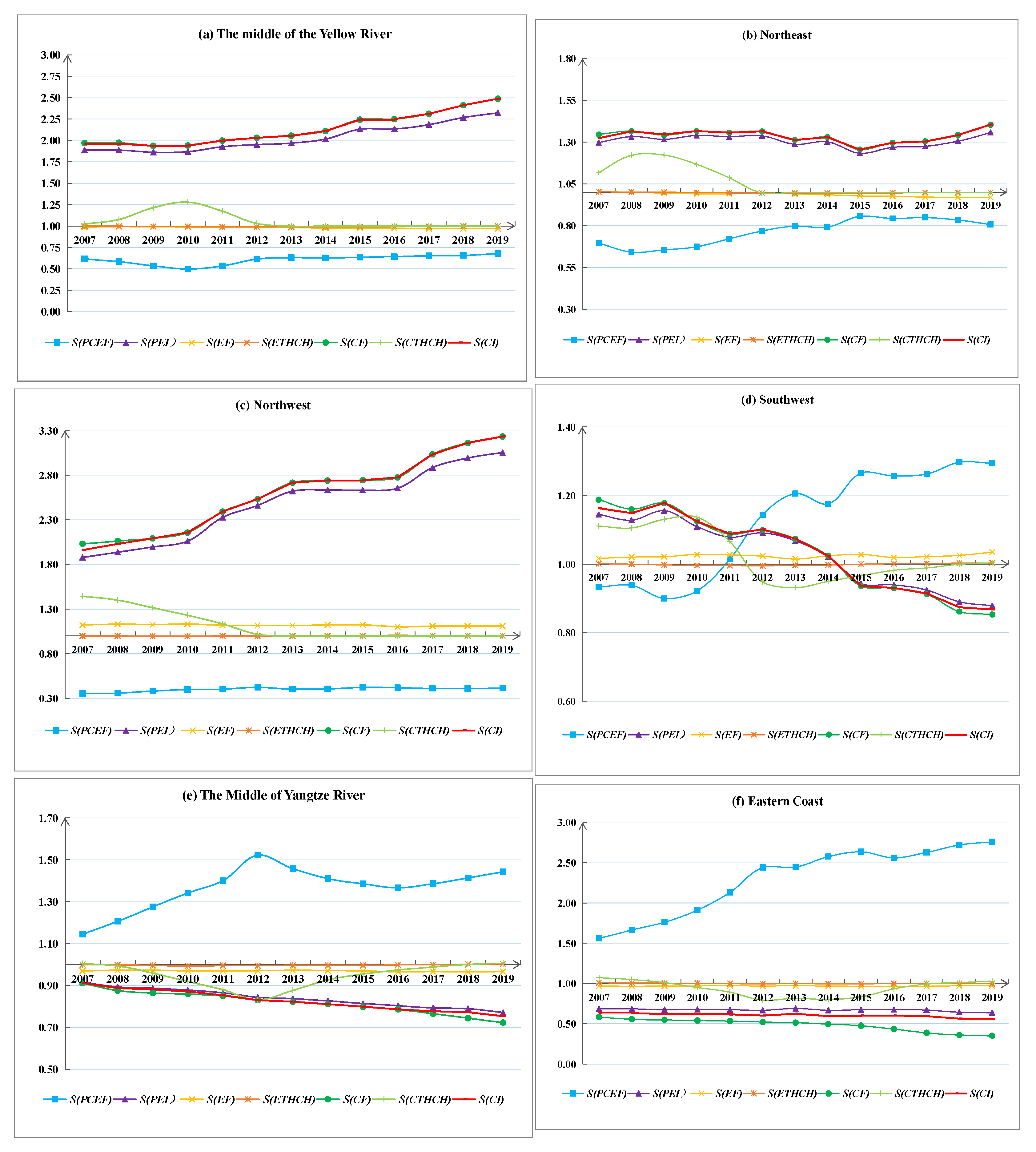
The variation in carbon intensity in the different regions of China increased each year. Specifically, the northwest performed the worst in reducing carbon intensity, while the northern coast, the middle of Yellow River and the northeast regions also performed worse than the national average. Specific to the factors, these regions consciously improved carbon emission technology (CTHCH), but their carbon emission efficiency was not significantly improved to reduce CI. The northwest region exhibited poor performance in the ability for PEI and CF factors to reduce CI, which remains significantly lower than the national average level. On the contrary, the southwest represented by Sichuan and Chongqing made great efforts to improve carbon emission technology (CTHCH), increase CF, and reduce EI by constantly catching up with carbon emission reduction technologies in advanced regions. The CI of the eastern coast and the middle of Yangtze River was always lower than the national average level, and its CI basically decreased by 2–3% per year. Specifically, it maintained the stability of the rate of CI by maintaining CF and EI. The central region exhibited poor performance on CTHCH, and the northeast region performed poorly in EF. In addition, the eastern coastal region exhibited poor performance in CTHCH and CF.

(3)

At the province level, the growth of the carbon intensity in Ningxia, Shandong, Xinjiang, Liaoning, Yunnan, Gansu, Hebei, Qinghai, Jilin, and Shaanxi was greater than the average growth, and the spatial differences in the carbon intensity in Ningxia, Xinjiang, and Qinghai increased gradually over time. It is necessary to take measures to control the serious state of the carbon intensity in these provinces. In particular, Ningxia and Qinghai exhibited poor performance in reducing the carbon intensity of PEI factors, while other provinces, such as Shandong, Xinjiang, and Hebei, exhibited poor performance in CF and EF.

Based on the above research results, some policy implications can be put forward. First, energy intensity is a dominant factor in reducing the carbon intensity, and the northwest and the middle of the Yellow River have poor performance. Therefore, it is necessary to improve energy intensity by learning advanced technologies from developed areas. Second, the carbon emission efficiency is generally poor in China, except in the Jingjin areas and the southern coast. For energy efficiency, the northern coast and central regions have poor energy efficiency because of the resource-dependent development model. Therefore, it is necessary to change the development model and use new energy technologies to improve energy efficiency. Third, the regional disparities in technological efficiency progress in carbon emissions and energy usage in China are relatively small, which proves that development potential exists in this region. In particular, the magnitude of technological progress in the northwest and central regions is small. Therefore, it is necessary to enhance the concept of advanced technology absorption in the northwestern region and adopt corresponding financial or policy support to help more enterprises join the northwestern region in a cooperative manner, thereby improving its technological efficiency.

References

1. European Commission. Emission Database for Global Atmospheric Research. Joint Research Centre (JRC)/PBL Netherlands Environmental Assessment Agency. 2021. Available online: http://edgar.jrc.ec.europa.eu (accessed on 16 September 2022).
2. The State Council Information Office of the People’s Republic of China. Enhanced Actions on Climate Change: China’s Intended Nationally Determined; China’s State Council: Beijing, China, 2015. Available online: http://english.www.gov.cn/archive/publications/2015/07/01/content_281475138245408.htm (accessed on 1 July 2015).
3. Liang, Y.; Cai, W.; Ma, M. Carbon dioxide intensity and income level in the Chinese megacities’ residential building sector: Decomposition and decoupling analyses. Sci. Total Environ. 2019, 677, 315–327. [Google Scholar] [CrossRef] [PubMed]
4. Liu, N.; Ma, Z.; Kang, J. Changes in carbon intensity in China’s industrial sector: Decomposition and attribution analysis. Energy Policy 2015, 87, 28–38. [Google Scholar] [CrossRef]
5. Zhou, X.; Zhou, D.; Wang, Q. Who shapes China’s carbon intensity and how? A demand-side decomposition analysis. Energy Econ. 2020, 85, 104600. [Google Scholar] [CrossRef]
6. Li, J.; Meng, G.; Li, C.; Du, K. Tracking carbon intensity changes between China and Japan: Based on the decomposition technique. J. Clean. Prod. 2022, 349, 131090. [Google Scholar] [CrossRef]
7. Wang, S.; Xie, Z.; Wu, R.; Feng, K. How does urbanization affect the carbon intensity of human well-being? A global assessment. Appl. Energy 2022, 312, 118798. [Google Scholar] [CrossRef]
8. Yang, L.; Xia, H.; Zhang, X.; Yuan, S. What matters for carbon emissions in regional sectors? A China study of extended STIRPAT model. J. Clean. Prod. 2018, 180, 595–602. [Google Scholar] [CrossRef]
9. Zhang, S.; Zhao, T. Identifying major influencing factors of CO2 emissions in China: Regional disparities analysis based on STIRPAT model from 1996 to 2015. Atmos. Environ. 2019, 207, 136–147. [Google Scholar] [CrossRef]
10. Xu, S.C.; He, Z.X.; Long, R.Y.; Chen, H.; Han, H.M.; Zhang, W.W. Comparative analysis of the regional contributions to carbon emissions in China. J. Clean. Prod. 2016, 127, 406–417. [Google Scholar] [CrossRef]
11. Yan, Q.; Zhang, Q.; Zou, X. Decomposition analysis of carbon dioxide emissions in China’s regional thermal electricity generation, 2000–2020. Energy 2016, 112, 788–794. [Google Scholar] [CrossRef]
12. Sun, W.; Wang, C.; Zhang, C. Factor analysis and forecasting of CO2 emissions in Hebei, using extreme learning machine based on particle swarm optimization. J. Clean. Prod. 2017, 162, 1095–1101. [Google Scholar] [CrossRef]
13. Chang, Y.F.; Lin, S.J. Structural decomposition of industrial CO2 emission in Taiwan: An input-output approach. Energy Policy 1998, 26, 5–12. [Google Scholar] [CrossRef]
14. Chang, N.; Lahr, M.L. Changes in China’s production-source CO2 emissions: Insights from structural decomposition analysis and linkage analysis. Econ. Syst. Res. 2016, 28, 224–242. [Google Scholar] [CrossRef]
15. Wang, Z.; Liu, W.; Yin, J. Driving forces of indirect carbon emissions from household consumption in China: An input–output decomposition analysis. Nat. Hazards 2015, 75, 257–272. [Google Scholar] [CrossRef]
16. Chong, C.; Liu, P.; Ma, L.; Li, Z.; Ni, W.; Li, X.; Song, S. LMDI decomposition of energy consumption in Guangdong Province, China, based on an energy allocation diagram. Energy 2017, 133, 525–544. [Google Scholar] [CrossRef]
17. Lin, B.; Tan, R. Sustainable development of China’s energy intensive industries: From the aspect of carbon dioxide emissions reduction. Renew. Sustain. Energy Rev. 2017, 77, 386–394. [Google Scholar] [CrossRef]
18. Duan, C.; Chen, B.; Feng, K.; Liu, Z.; Hayat, T.; Alsaedi, A.; Ahmad, B. Interregional carbon flows of China. Appl. Energy 2018, 227, 342–352. [Google Scholar] [CrossRef]
19. Wang, M.; Feng, C. Decomposing the change in energy consumption in China’s nonferrous metal industry: An empirical analysis based on the LMDI method. Renew. Sustain. Energy Rev. 2018, 82, 2652–2663. [Google Scholar] [CrossRef]
20. Zhang, C.; Su, B.; Zhou, K.; Yang, S. Analysis of electricity consumption in China (1990–2016) using index decomposition and decoupling approach. J. Clean. Prod. 2019, 209, 224–235. [Google Scholar] [CrossRef]
21. Zhou, P.; Ang, B.W. Decomposition of aggregate CO2 emissions: A production-theoretical approach. Energy Econ. 2008, 30, 1054–1067. [Google Scholar] [CrossRef]
22. Wang, Q.; Han, X.; Li, R. Does technical progress curb India’s carbon emissions? A novel approach of combining extended index decomposition analysis and production-theoretical decomposition analysis. J. Environ. Manag. 2022, 310, 114720. [Google Scholar] [CrossRef]
23. Li, H.; Zhao, Y.; Qiao, X.; Liu, Y.; Cao, Y.; Li, Y.; Wang, S.; Zhang, Z.; Zhang, Y.; Wang, J. Identifying the driving forces of national and regional CO2 emissions in China: Based on temporal and spatial decomposition analysis models. Energy Econ. 2017, 68, 522–538. [Google Scholar] [CrossRef]
24. Zhou, P.; Zhang, H.; Zhang, L. The drivers of energy intensity changes in Chinese cities: A production-theoretical decomposition analysis. Appl. Energy 2022, 30, 118230. [Google Scholar] [CrossRef]
25. Tian, Y.; Wang, Y.Z.; Hang, Y.; Wang, Q.W. The two-stage factors driving changes in China’s industrial SO2 emission intensity: A production-theoretical decomposition analysis. Sci. Total Environ. 2021, 814, 152426. [Google Scholar] [CrossRef] [PubMed]
26. Chen, L.; Duan, Q. Decomposition analysis of factors driving CO2 emissions in Chinese provinces based on production-theoretical decomposition analysis. Nat. Hazards 2016, 84 (Suppl. 1), 267–277. [Google Scholar] [CrossRef]
27. Liu, B.; Shi, J.; Wang, H.; Su, X. Driving factors of carbon emissions in China: A joint decomposition approach based on meta-frontier. Appl. Energy 2019, 256, 113986. [Google Scholar] [CrossRef]
28. Zhang, Y.; Yu, Z.; Zhang, J. Research on carbon emission differences decomposition and spatial heterogeneity pattern of China’s eight economic regions. Environ. Sci. Pollut. Res. Int. 2022, 29, 29976–29992. [Google Scholar] [CrossRef]
29. Banerjee, S. Addressing the carbon emissions embodied in India’s bilateral trade with two eminent Annex-II parties: With input–output and spatial decomposition analysis. Environ. Dev. Sustain. 2020, 23, 5430–5464. [Google Scholar] [CrossRef]
30. Guo, B.; Geng, Y.; Franke, B.; Hao, H.; Liu, Y.; Chiu, A. Uncovering China’s transport CO2 emission patterns at the regional level. Energy Policy 2014, 74, 134–146. [Google Scholar] [CrossRef]
31. Pothen, F.; Schymura, M. Bigger cakes with fewer ingredients? A comparison of material use of the world economy. Ecol. Econ. 2015, 109, 109–121. [Google Scholar] [CrossRef]
32. Mundaca, L.; Markandya, A. Assessing regional progress towards a ‘green energy economy’. Appl. Energy 2016, 179, 1372–1394. [Google Scholar] [CrossRef]
33. Ang, B.W.; Zhang, F.Q. Inter-regional comparisons of energy-related CO2 emissions using the decomposition technique. Energy 1999, 24, 297–305. [Google Scholar] [CrossRef]
34. Ang, B.W.; Xu, X.; Su, B. Multi-country comparisons of energy performance: The index decomposition analysis approach. Energy Econ. 2015, 47, 68–76. [Google Scholar] [CrossRef]
35. Román-Collado, R.; Morales-Carrión, A.V. Towards sustainable growth in Latin America: A multiregional spatial decomposition analysis of the driving forces behind CO2 emissions changes. Energy Policy 2018, 115, 273–280. [Google Scholar] [CrossRef]
36. Yuan, R.; Rodrigues, J.F.D.; Behrens, P. Driving forces of household carbon emissions in China: A spatial decomposition analysis. J. Clean. Prod. 2019, 233, 932–945. [Google Scholar] [CrossRef]
37. Zhou, B.; Zhang, C.; Song, H.; Wang, Q. How does emission trading reduce China’s carbon intensity? An exploration using a decomposition and difference-in-differences approach. Sci. Total Environ. 2019, 676, 514–523. [Google Scholar] [CrossRef]
38. Chen, J.; Xu, C.; Cui, L.; Huang, S.; Song, M. Driving factors of CO2 emissions and inequality characteristics in China: A combined decomposition approach. Energy Econ. 2019, 78, 589–597. [Google Scholar] [CrossRef]
39. Wang, H.; Ang, B.W.; Su, B. A Multi-region Structural Decomposition Analysis of Global CO2 Emission Intensity. Ecol. Econ. 2017, 142, 163–176. [Google Scholar] [CrossRef]
40. Zhang, C.; Wu, Y.; Yu, Y. Spatial decomposition analysis of water intensity in China. Soc.-Econ. Plan. Sci. 2019, 69, 100680. [Google Scholar] [CrossRef]
41. Wang, H.; Zhou, P. Multi-country comparisons of CO2 emission intensity: The production-theoretical decomposition analysis approach. Energy Econ. 2018, 74, 310–320. [Google Scholar] [CrossRef]
42. Ang, B.W.; Su, B.; Wang, H. A spatial–temporal decomposition approach to performance assessment in energy and emissions. Energy Econ. 2016, 60, 112–121. [Google Scholar] [CrossRef]
43. Chen, L.; Yang, Z. A spatio-temporal decomposition analysis of energy-related CO2 emission growth in China. J. Clean. Prod. 2015, 103, 49–60. [Google Scholar] [CrossRef]
44. Liu, X.; Peng, R.; Zhong, C.; Wang, M.; Guo, P. What drives the temporal and spatial differences of CO2 emissions in the transport sector? Empirical evidence from municipalities in China. Energy Policy 2021, 159, 112607. [Google Scholar] [CrossRef]
45. Meng, B.; Wang, J.G.; Andrew, R.; Xiao, H.; Xue, J.; Peters, G.P. Spatial spillover effects in determining China’s regional CO2 emission growth: 2007–2010. Energy Econ. 2016, 63, 161–173. [Google Scholar] [CrossRef]
46. Hang, Y.; Wang, Q.; Wang, Y.; Su, B.; Zhou, D. Industrial SO2 emissions treatment in China: A temporal-spatial whole process decomposition analysis. J. Environ. Manag. 2019, 243, 419–434. [Google Scholar] [CrossRef] [PubMed]
47. Kim, K.; Kim, Y. International comparison of industrial CO2 emission trends and the energy efficiency paradox utilizing production-based decomposition. Energy Econ. 2012, 34, 1724–1741. [Google Scholar] [CrossRef]
48. Färe, R.; Grosskopf, S.; Lovell, C.K.; Pasurka, C. Multilateral productivity comparisons when some outputs are undesirable: A nonparametric approach. Rev. Econ. Stat. 1989, 71, 90–98. [Google Scholar] [CrossRef]
49. Chung, Y.H.; Färe, R.; Grosskopf, S. Productivity and undesirable outputs: A directional distance function approach. J. Environ. Manag. 1997, 51, 229–240. [Google Scholar] [CrossRef] [Green Version]
50. IPCC. IPCC Guidelines for National Greenhouse Gas Inventories. 2006. Available online: https://www.ipcc-nggip.iges.or.jp/public/2006gl/chinese/index.html (accessed on 10 October 2014).
Figure 1. The carbon intensity (CI) changes in 30 provinces from 2007–2019.
Sustainability 14 12359 g001
Figure 2. (a) The cumulative change in CI in eight regions from 2007 to 2019. (b) The cumulative effects of CI driving factors in China from 2007 to 2019.
Sustainability 14 12359 g002
Figure 3. The cumulative spatial decomposition results and spatial disparities in eight regions (2007–2019).
Sustainability 14 12359 g003
Figure 4. The dynamic spatial decomposition results over time in the eight regions.
Sustainability 14 12359 g004aSustainability 14 12359 g004b
Figure 5. The cumulative spatial decomposition result in 30 provinces during 2007–2019.
Sustainability 14 12359 g005
Figure 6. The cumulative temporal–spatial decomposition results for each factor in the eight regions (2007–2019).
Sustainability 14 12359 g006
Figure 7. The change trends of the temporal–spatial decomposition results in eight regions.
Sustainability 14 12359 g007
Figure 8. The cumulative temporal–spatial decomposition results for each factor in 30 provinces (2007–2019).
Sustainability 14 12359 g008
Publisher’s Note: MDPI stays neutral with regard to jurisdictional claims in published maps and institutional affiliations.