Curve-Aware Model Predictive Control (C-MPC) Trajectory Tracking for Automated Guided Vehicle (AGV) over On-Road, In-Door, and Agricultural-Land

Abstract

Navigating the AGV over the curve path is a difficult problem in all types of navigation (landmark, behavior, vision, and GPS). A single path tracking algorithm is required to navigate the AGV in a mixed environment that includes indoor, on-road, and agricultural terrain. In this paper, two types of proposed methods are presented. First, the curvature information from the generated trajectory (path) data is extracted. Second, the improved curve-aware MPC (C-MPC) algorithm navigates AGV in a mixed environment. The results of the real-time experiments demonstrated that the proposed curve finding algorithm successfully extracted curves from all types of terrain (indoor, on-road, and agricultural-land) path data with low type 1 (percentage of the unidentified curve) and type 2 (extra waypoints added to identified curve) errors, and eliminated path noise (hand-drawn line error over map). The AGV was navigated using C-MPC, and the real-time and simulation results reveal that the proposed path tracking technique for the mixed environment (indoor, on-road, agricultural-land, and agricultural-land with slippery error) successfully navigated the AGV and had a lower RMSE lateral and longitudinal error than the existing path tracking algorithm.

1. Introduction

The Automatic Guided Vehicle (AGV) is used in many kinds of applications. They have done many kinds of important tasks in the field of indoor transportation [1,2,3], movement of outdoor goods [4,5], as well as agricultural [6,7] works. The AGV follows a predefined path that can be navigated using landmarks-based, behavior-based, vision-based, and GPS-based navigation [8]. The AGV has been navigated across the fixed navigating medium on a floor, which is wire type and guide type, for landmarks-based navigation. Wired navigation [9] makes use of a slit or wire that is cut and inserted beneath the surface. A sensor is mounted at the bottom of the AGV to determine the position based on the radio signal being transmitted to the wire. This information is used for the steering circuit, which assists the AGV in following the path. The camera in a guide-type [10] sensor vehicle follows the path of a tape or painted line. For mobility, the behavioral navigation system employs laser beam navigation technology. In the system, laser beam navigation technology [11] is utilized to calculate vehicle position and navigation. Laser navigation is often regarded as the most effective and efficient approach for avoiding obstacles and following a path. It moves without the use of cables, rails, or tracks. A beam is transmitted and received from a sensor; the time it takes for the beam to travel and return helps in measuring distance and angle, which helps the vehicle’s motion. The present pose of the AGV is then compared to an already installed map in the AGV’s memory. The navigation is connected with the external sensor that takes information from the workspace by measuring proximity and visual image, according to vision-based navigation [12]. Vision-based AGVs use a camera to acquire environmental data and make decisions based on those features to steer the vehicle. According to GPS [13] navigation, GPS receiver data has been used to compute with Google map coordinates data. The AGV has navigated based on the computation.

1.1. Problem Analysis and Motivation

The Automatic Guided Vehicle follows a predetermined path at a constant speed. The AGV struggles whenever it approaches the curvature area on the path. When the AGV operates on agricultural land and is not aware of path curvature, it achieves a Mean Absolute Error (MAE) [14] of 0.1947 m error, indicating that the AGV is going away from the ground truth path [15], due to the AGV speed being steady if the AGV speed has increased. D. Puppim de Oliveira et al. [16] tested the AGV in an indoor environment using landmark-based navigation and discovered a curvature path on a tape-type path. They increased the AGV’s speed and stated that the experiment meets to identify the motion blur occurrence in the speed range of 0.08 m/s to 0.29 m/s, as well as its impact on measurements. In this study, it is proposed to navigate the AGV at the appropriate speed along a curved course, as well as to travel over a combined path of indoor, on-road, and agricultural terrain.

Figure 1 depicts the AGV parking in the indoor (shed) and needing to navigate the indoor (green path) and go over the on-road path (blue line) before arriving on agricultural land and performing an agricultural activity (brown path). There are 17 curves in this composite path (a combination of green, blue, and brown paths). In this scenario, the AGV should move slowly indoors and in agricultural areas (2 to 3 km/h) and quickly (7 to 15 km/h) on the road. When the path tracking algorithm navigates the AGV, which approaches a curvature in its course, the current speed must be decreased based on the radius of curvature.

1.2. Related Work

The existing curve-aware AGV is P. T.-T. Nguyen et al. [17] offer an updated Pure Pursuit algorithm such that the AGV can predict the trajectory and slow down for turning, improving path tracking accuracy. They used LiDAR with SLAM technology for indoor navigation. Wu et al. [18] encountered difficult issues for a vision-based AGV operating in a complicated workspace, such as non-uniform lighting, sight-line occlusion, or stripe damage, which unavoidably resulted in incomplete or deformed route pictures as well as numerous fake artifacts. To address this issue, they presented approaches based on Kernel Principal Component Analysis and a Back Propagation Neural Network (KPCA–BPNN) and Improved Particle Swarm Optimization and a Binary Tree Guidance Window Partition (IPSO–BTGWP). The curvilinear pathways were distinguished from their straight counterparts using a path classifier based on KPCA–BPNN. J.H. Han et al. [19] used a feature point extraction technique with LRF calibration and amplification errors dependent on the materials and colors of the asphalt and lanes to create a laser-scanned 3D road map and to identify and recognize lanes. The test results revealed that using their method could assure safe driving under poor road conditions, such as fog and curvature paths, which might help in the research and development of autonomous driving technologies.

The LiDAR costs between 5348 USD and 103,904 USD, according to the S. Bi et al. [20] study, depending on the configuration range. C. Medina Sánchez et al. [21] reviewed the camera cost range from 149 USD to 449 USD, which may be used for RGB and RGB-D purposes in autonomous mobile robots. A. A. Süzen et al. [22] studied image processing embedded boards and discovered that the Raspberry Pi 4 costs $35, the Jetson Nano costs $89, and the Jetson TX2 costs $399.

In navigation of agricultural land, an approach presented by J. Bengochea-Guevara et al. [23] combines a camera and a GPS receiver to get a set of basic behaviors necessary for an autonomous mobile robot to survey a crop field in its entirety. Vision-guided navigation was also achieved through the development of two fuzzy controllers. The robot’s row-changing maneuvers (steering across a curve path) were established. However, the author had to contend with the noise and disruption caused by mobile robots, which are widespread in the agricultural sector. In the context of AGV disturbance, Zhengduo Liu et al. [24] thoroughly examined and verified the robust stability of agricultural vehicles. The results showed that when the trajectory equation was altered or a disturbance was introduced, the controller could respond quickly, allowing the vehicle to return to the reference track as soon as possible.

According to curvature in GPS navigation path, the proposed technique by J Han et al. [25] is based on the usage of a low-cost Global Navigation Satellite System and a Real-Time Kinematic (GNSS-RTK) module and a low-cost motion sensor module that includes positioning and path-tracking control algorithms. Three waypoint-based trajectories were used to evaluate performance: straight-line parts, curve sections, and in-situ rotation sections. They found that it is important to incorporate an adjustable search radius for enclosed-based line-of-sight (LOS) guidance depending on the turning radius at various curve paths to improve path-following performance in the curve section.

In the scenario of obtaining a horizontal curve using Google map path data, Li et al. [26] offer a fully automated approach for extracting horizontal curve data from GIS road maps. The suggested method aims to accomplish four things. (a) From each road, detect all curves in the selected layers of the roadway, independent of curve type. (a) Classify each curve into one of two categories: simple or compound. (c) Automatically calculate the radius and degree of curvature of each simple curve, as well as the lengths of simple and compound curves. (d) Create curve characteristics and layers in the GIS for all recognized curves automatically. A total of 96.7% of curves were correctly detected and geometric information was computed using the proposed technique. Road Curvature Analyst (ROCA) [27] software by Bil et al. defined the horizontal curve of a road segment and automatically determined the curve radius and azimuth. They utilized the Bayes classifier for curve recognition. The ROCA software reduced noisy segments using the Douglas–Pecker generalization process.

The most prevalent path-tracking algorithms are pure pursuit [28], Stanley [29], Least Quadratic Regulator (LQR) [30], and Model Predictive Control (MPC) [31,32,33].

1.3. Contribution

This work focused on the AGV’s path tracking algorithm on curve paths and navigating the AGV in various terrains: in-door, on-road, and agricultural. The following are the primary contributions of our work:

• The proposed curve finding algorithm is used to locate curves in Google map data and to Find the properties (curve radius, starting and ending points, and speed limit) of the extracted curve;
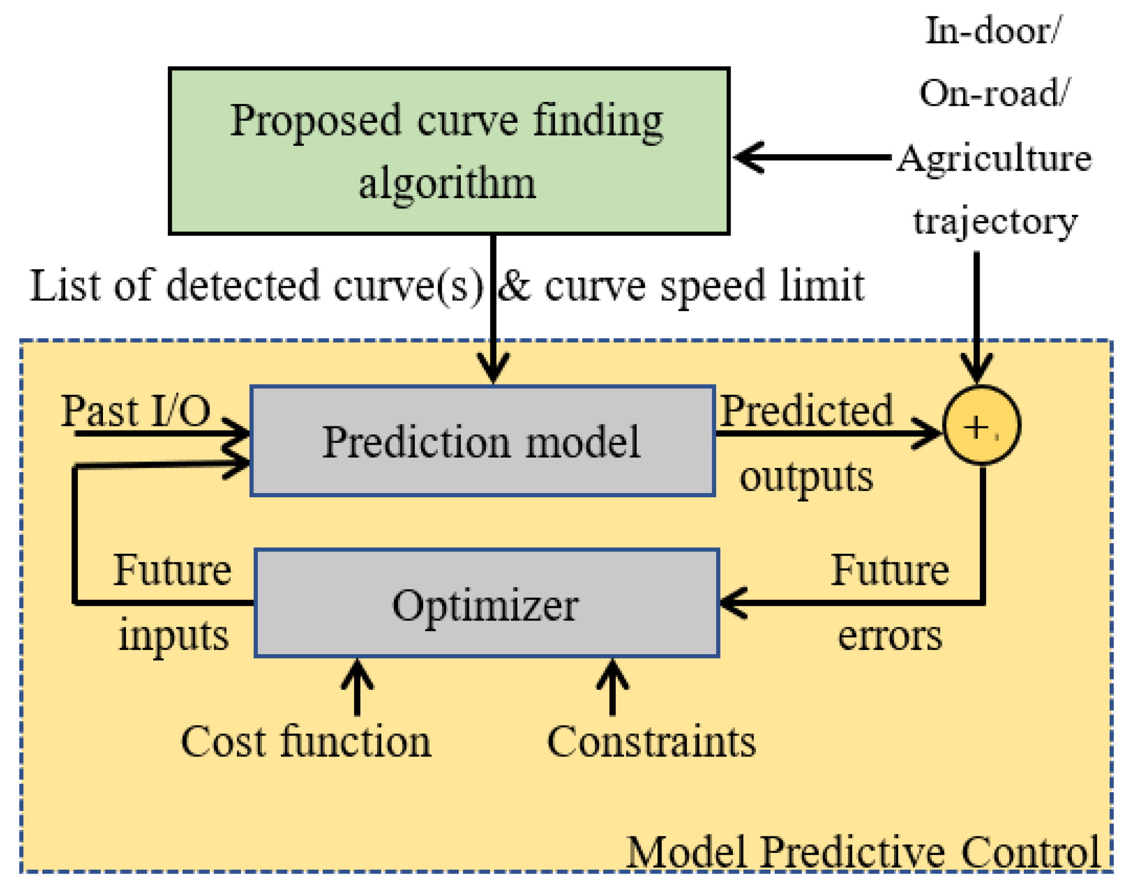
• The Model Predictive Control (MPC) technique is employed in the path tracking algorithm to improve the awareness of an oncoming curve. The predictive model of the MPC has loaded a list of upcoming curves on the course and has drawn up a future path that is aware of curvature. The enhanced MPC algorithm must reduce the AGV speed based on the curve speed limit;
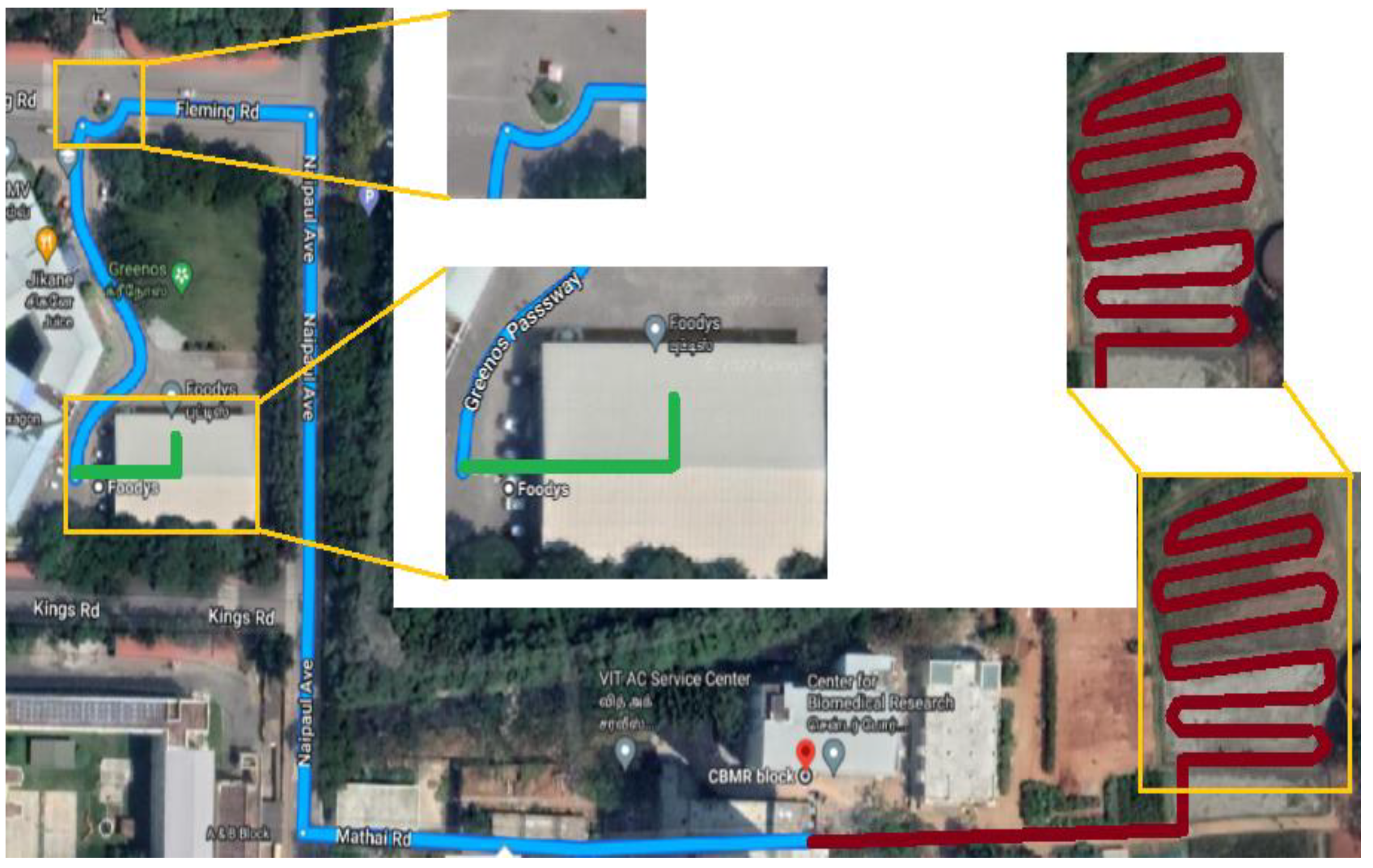
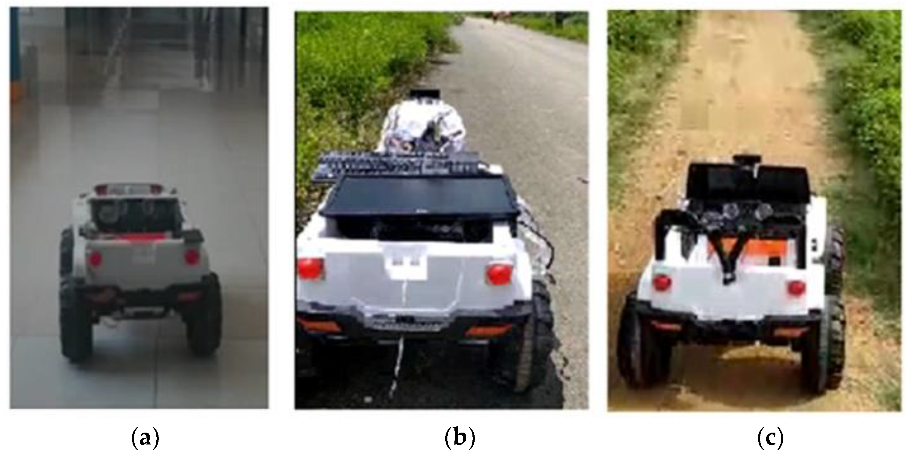
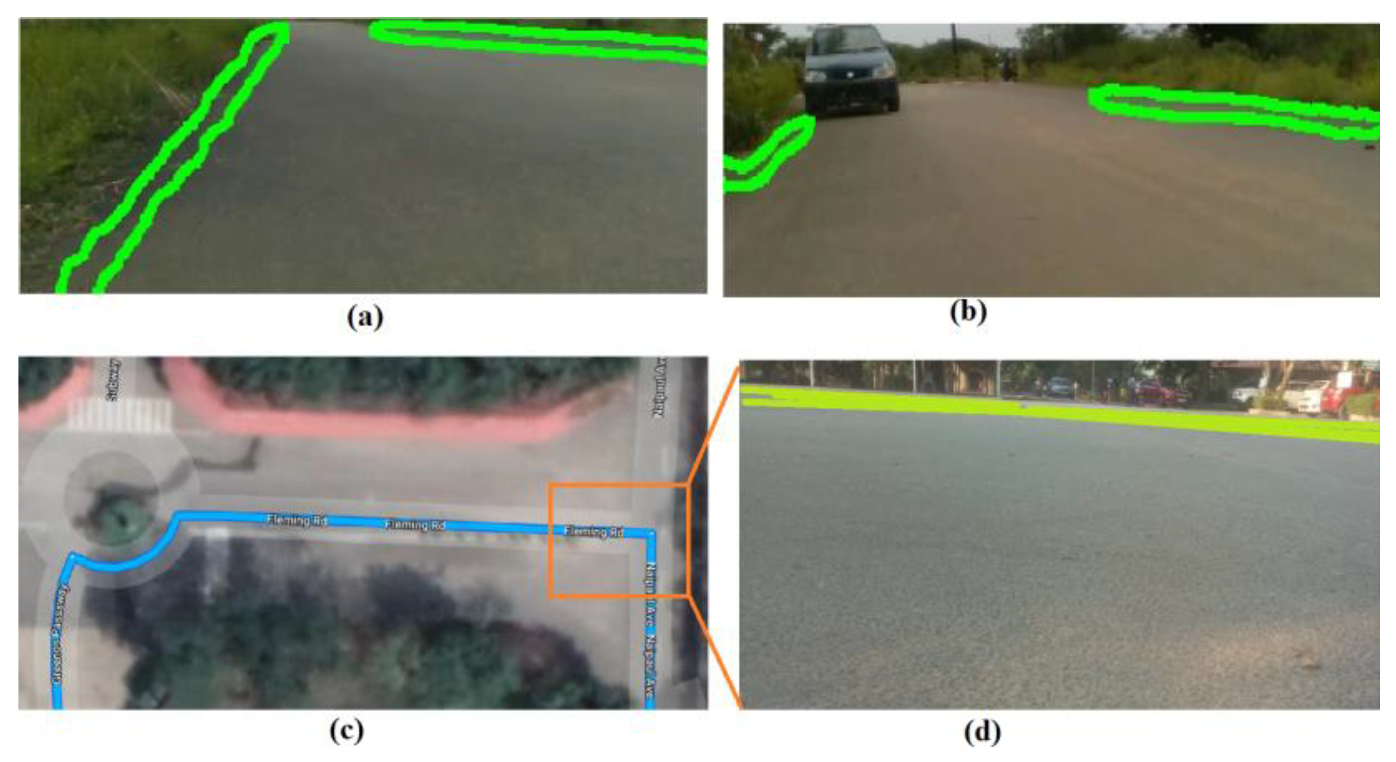
• In addition, practical experiments on the in-door, on-road, and agricultural paths depicted in Figure 1 are carried out to ensure that the proposed system is feasible.

The rest of this work is arranged in the following manner. The hardware platform, Odometry Motion Model, Noise Model for Odometry, Non-GPS location update, proposed curve finding technique, and upgrade MPC as curve-aware MPC (C-MPC) are all discussed in Section 2. Section 3 discusses the results of the proposed curve finding and C-MPC in real-time and simulation. Finally, Section 4 discusses the conclusion.

2. Proposed Model

The proposed curve-aware MPC algorithm block diagram is shown in Figure 2. The system retrieves horizontally curved road information from the indoor/agricultural/on-road Google map path waypoint using the proposed curve-finding approach. The radius of the curve is then used to construct a curve speed limit database. The retrieved curve information is then entered into the MPC algorithms prediction model, along with the curve speed limit. The prediction model reduces the vehicle’s speed as it approaches the curve.

2.1. Automated Guided Vehicle (AGV) Architecture

The proposed AGV architecture is shown in Figure 3. The front and rear DC motor specifications are Speed (N) 15,000 RPM, Voltage 15 V, and Current 0.65 A. Using the Arduino UNO controller, the rear and front DC motors are controlled. The battery supply voltage is 7.2 V for the DC motor and 7 A for the current. A 5 V 10 A two-channel relay is used instead of a motor drive, as the current supplied by the relay is higher compared to the engine drive. This also offers the benefit of stopping the engine from having an excessive continuous power supply. For Raspberry pi and Arduino UNO, there is a separate power bank supply powered by a Philips 20,000 Mah power bank. The LM393 Hall Effect sensor and MPU9250 IMU sensors are integrated with the Raspberry pi. The embedded board of the Raspberry pi receives IMU and Hall effect sensor data as input and provides the output steering angle.

The computed values of the steering angle are transferred to the Arduino UNO controller for steering and forwarding controls. AGV steering angle movement is 15° to 165° and must be divided into 5 parts. Angles 15° to 45° are an absolute right angle, angles 45° to 75° are a right angle, angles 75° to 105° are a forward angle, angles 105° to 135° are a left angle, and angles 135° to 165° are an absolute left angle. The AGV is unable to transform 15° to 0° (right) and 165° to 180° (left) angles due to the hardware control limitation, as shown in Figure 4.

The Arduino UNO controls both the steering angle and the forward movement. The backward movement facility has been truncated because the AGV has no computation at its backward side. The speed of a non-payload vehicle is 15.5 Km/h. The payload speed of the vehicle (10 kg–15 kg) ranges from 12.5 Km/h to 9 Km/h, depending on the weight of the payload.

The AGV’s moving distance can be measured using two LM393 Hall Effect sensors. The radius of the wheel is 0.145 m and the diameter is 0.9144 m (3 feet) so that one Hall Effect Sensor can detect one rotation in 3 feet and then, using two Hall Effect Sensors (in opposite direction), one can detect one rotation per 1.5 feet on the basis that one can measure the speed of the AGV. The moving direction of the AGV is derived from the MPU9250 IMU sensor. The sensor is equipped with an accelerometer, a gyroscope, and a magnetometer. The three axes of the magnetometer are pitch, roll, and yaw. The value of the yaw is used to measure the direction of the AGV.

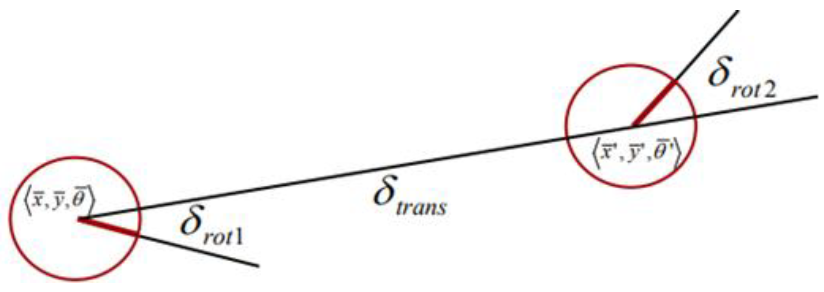
2.2. Odometry Motion Model [34]

Odometry is generally accomplished by integrating information from wheel encoders; most commercial robots provide such integrated pose estimation at repeated time periods. Figure 5 shows the AGV moves from the <$\overline{x},\overline{y},\overline{\theta }$> location to <$\overline{x\prime },\overline{y\prime },\overline{\theta \prime }$> location using odometry information $u=<{\delta }_{rot1},{\delta }_{trans},{\delta }_{rot2}>$ where the initial turn is called ${\delta }_{rot1}$, the translation ${\delta }_{trans}$, and the second rotation ${\delta }_{rot2}$. Each of them is calculated as the following equation.

$${\delta }_{trans}=\sqrt{{(\overline{x^{\prime }}-\overline{x})}^2+{(\overline{y^{\prime }}-\overline{y})}^2}$$

(1)

$${\delta }_{rot1}=atan2(\overline{y^{\prime }}-\overline{y}, \overline{x^{\prime }}-\overline{x})-\overline{\theta }$$

(2)

$${\delta }_{rot2}=\overline{\theta \prime }-\overline{\theta }-{\delta }_{rot1}$$

(3)

2.3. Noise Model for Odometry

To model the motion error [34], we assume that the “true” values of the rotation and translation are obtained from the measured ones by subtracting independent noise ${\epsilon }_b$ with zero mean and variance b (e.g., with normal or triangular distribution):

$${\widehat{\delta }}_{rot1}={\delta }_{rot1}-{\epsilon }_{{\alpha }_1 \left|{\delta }_{rot1}\right|+{\alpha }_2 \left|{\delta }_{trans}\right|}$$

(4)

$${\widehat{\delta }}_{trans}={\delta }_{trans}-{\epsilon }_{{\alpha }_3 \left|{\delta }_{trans}\right|+{\alpha }_4\left( \left|{\delta }_{rot1}+{\delta }_{rot2}\right|\right)}$$

(5)

$${\widehat{\delta }}_{rot2}={\delta }_{rot2}-{\epsilon }_{{\alpha }_1 \left|{\delta }_{rot2}\right|+{\alpha }_2 \left|{\delta }_{trans}\right|}$$

(6)

The parameters ${\alpha }_1$ to ${\alpha }_4$are robot-specific error parameters, which specify the error accrued with motion.

2.4. Non-GPS Location Update

When the GPS is failed in some locations, this non-GPS location calculation is active. Here, IMU’s orientation data is used. The orientation sensor has three axes Pitch, Roll, and Yaw. Here the Yaw is the direction in 360 degrees. This Yaw value is used as a bearing in the calculation. From the wheel rotation sensor, the distance traveled is calculated as follows:

If the diameter of the two-wheeler wheel is $di$, then the circumference is calculated as $cr=di\times \pi$ and then the distance travelled is $dst=cr\times cu$, where $cu$ is wheel rotation count. Let the GPS has failed to receive the current signal but have the previous location signal as $latitud{e}_{previous}$ and $longitud{e}_{previous}$. Now, compute the present latitude and longitude. Let R = 6378.1 km be the radius of the earth. If the bearing value is gotten from the IMU sensor (Orientation sensor Yaw axis), then the calculation is.

$$\begin{array}{ll}latitud{e}_{present}& ={\sin }^{-1}(\sin (latitud{e}_{previous})\\ & \times \cos \left(\frac{dst}{R}\right)+\cos (latitud{e}_{previous})\\ & \times \sin \left(\frac{dst}{R}\right)\times \cos \left(bearing\right))\end{array}$$

(7)

$$\begin{array}{l}longitude{t}_{present}\\ =longitud{e}_{previous}\\ +{\tan }^{-1}\frac{(\sin \left(bearing\right) \times \sin \left(\frac{dst}{R}\right) \times \cos (latitud{e}_{previous})}{\cos (\frac{dst}{R}) - \sin (latitud{e}_{previous}) \times \sin (nex{t}_{latitude})}\end{array}$$

(8)

Hence, the $latitud{e}_{present}$ and $longitude{t}_{present}$ values are used to update AGV location.

2.5. Trajectory (Path) Creation

Before navigating the AGV, the trajectory must be created. The values for the starting point’s latitude and longitude are required for trajectory creation. The non-GPS location update (Section 2.4) method described in the previous section is used to generate each waypoint of the trajectory (path). This method is more suitable for generating indoor trajectories. During the indoor trajectory creation, the user manually navigated the AGV. The open-street map is used in outdoor settings, specifically on-road and agricultural land. Hand-drawn lines were drawn over an open-street map area to create this outdoor trajectory.

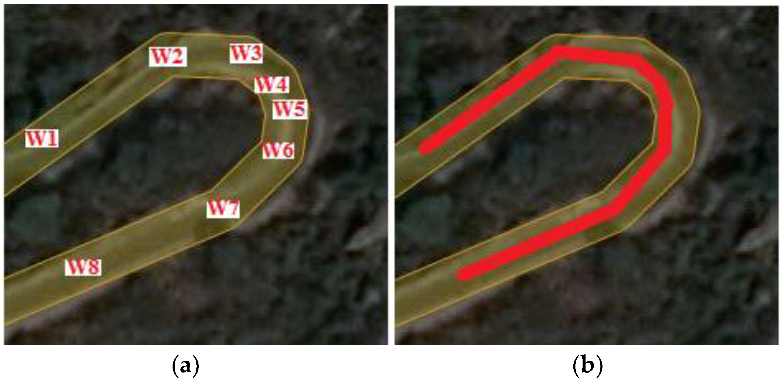
2.6. Proposed Curve Finding Algorithm

A path is built from the source location information to the destination location information. The path is depicted in Figure 6a as a set of waypoints (W1 to W8) connected by straight lines. The formula for calculating the curve using the waypoint sequence is shown below.

Let us first determine the distance between two waypoints before calculating the radius of curvature of the path. The great-circle distance between two places is calculated using the ‘haversine’ formula.

$$\mathrm{a}=\sin 2\left(\mathsf{\Delta }\mathsf{\phi }/2\right)+\cos \mathsf{\phi }1\times \cos \mathsf{\phi }2\times \sin 2\left(\mathsf{\Delta }\mathsf{\lambda }/2\right)$$

(9)

$$\mathrm{c}=2\times {\tan }^{-1}\frac{\sqrt{a}}{\sqrt{\left(1-a\right)}}$$

(10)

$$\mathrm{d}=\mathrm{R}\cdot \mathrm{c}$$

(11)

where $\mathsf{\phi }$ is latitude, $\mathsf{\lambda }$ is longitude, R is earth’s radius (R = 6371 km). Let us consider the distance between waypoint W1 to W2 as x, W2 to W3 as y, and W1 to W3 as z. Then, finding the radius is

$$radius=\frac{\left(x\times y\times z\right)}{\sqrt{\left(x+y+z\right)\times \left(y+z-x\right)\times \left(z+x-y\right)\times \left(x+y-z\right)}}$$

(12)

Assume the curve’s maximum radius is 200 m. Because the AGV is small in height and width, it moves at a slower speed (maximum speed of 15 km/h). The path with turns or a narrow curvature must be extracted. Every turn in the corridor is from the indoor path. The road in the outdoor environment has sharp turns or roundabouts, while the agricultural land has U-turns in each plant row. All of these turns or curves are within a radius of 200 m. The AGV moving in a curve must reduce its speed and can only move at the declared speed described in

Table 1. Curve speed limit database.

S.no	Radius of Curve Range	IRC Speed Limit for Vehicles	Declared Speed Limit for AGV	Curve Alert Location
1	50–100 m	20 km/h	3 km/h	5 m before the curve starting point
2	70–150 m	25 km/h	5 km/h	5 m before the curve starting point
3	100–200 m	30 km/h	7 km/h	5 m before the curve starting point

. A curve with a radius greater than 200 m is considered a straight path, and the AGV can move at full speed. Using Equation (12) for waypoints W1, W2, and W3 from Figure 6a, the radius of these three waypoints is less than 200 m because they appear to be on a curve. The radius value of these three waypoints is saved in the radius list and is checked against another adjacent waypoint until it reaches the path’s final waypoint. The waypoints W1–W8 in Figure 6a result in six curve radiuses Ri1, Ri2, Ri3, Ri4, Ri5, and Ri6, which were kept in the radius list. Finally, the average curve radius (Ri1 to Ri6) of the waypoints W1 to W8 is computed. Figure 6b depicts the identified curve of the path in Figure 6a. Algorithm 1 explains this in detail. The initial waypoint of the curve is W1, the ending waypoint is W8, the mid-waypoint is W4, and the average curve radius is all stored in the curve list.

Algorithm 1: Curve finding algorithm.

Input: GPS waypoints, radius in meter

Output: list of found curves and its properties

1: Function curve_finding(radius) 2:      for each waypoint from curve_points do 3:           x = distance of waypoints 1 and 2 4:           y = distance of waypoints 2 and 3 5:           z = distance of waypoints 1 and 3 6:           curve_radius = (x ∗ y ∗ z)/ 7:                                          (sqrt ((x + y + z) ∗ (y + z − x) ∗ (z + x − y) ∗ (x + y − z))) 8:           count = 0 9:            if curve radius ≤ radius_meters then: 10:                   curve_distance = curve_distance + (x + y) 11:                   total_radius = total_radius + curve_radius 12:                 count = count + 1 13:      else: 14:                   Radius = total_radius/count 15:      curve_List [radius, curve_distance] 16:      return curve_List 17: end Function 18: 19: list_curve_points = curve_finding(radius = 200) #200 m radius

The approach described above is applied to the path between the source and destination locations, and the identified curves and their properties (start point, endpoint, mid-point, and average radius) are kept in a curve list. The noise in the path refers to the non-uniformity of the connecting lines between the waypoints, as seen in Figure 7b yellow circle. The proposed curve detector approach can reduce this type of noise that is present inside the curve.

The creation of the curve speed limit database is simply in Indian roads supported by the reference of articles outlined by the Indian Road Congress (IRC) [35,36].

Table 1 depicts the planned speed limit vs. the radius of the curve as described in the Indian Road Congress (IRC) document. The radius range is determined by the curve’s super-elevation. Column 2 specifies the IRC speed limit for vehicles based on the radius of the curve. Because AGV moves slowly, this is not set, hence the defined speed limit for AGV is set in column 3. If the AGV approaches the curve before reaching the curve’s starting point, it must be alerted 5 m in advance.

2.7. Curve-Aware MPC (C-MPC) Design

The detected curve from the Google map path, together with its information and speed limits, is fed into the existing MPC algorithm prediction model. The current prediction model anticipates the AGV’s future action control until the prediction horizon distance value is reached (T). If T is set to seven, the future prediction is tested up to seven Google map waypoints. Algorithm 2 depicts the curve-aware prediction model.

The proposed method of this algorithm is found in lines 2–7, which concentrated on reducing the AGV’s speed (v) until it reached the curve speed limit. The prediction model function is given two parameters: a list of identified curves and their attributes (curve starting point, curve ending point, curve speed limit), and the location of the curve alert, where the curve alert location denotes five meters before the curve’s starting point.

Algorithm 2: Curve-aware prediction model algorithm.

Input: List of curves point, list of curve safe alert points

Output: The predicted control output. Abbreviation state: vehicle current state, T: prediction horizon value

1: function Prediction_model (list_of_curve_properties,curve_alert,T) 2:       for curve ∈ [list_of_curve_properties) do 3:           for i in range T: 4:                if (state.x < curve_start.x) and (state.y < curve_start.y) then: 5:                         if (state.x > curve_alert.x) and (state.y > curve_alert.y) then: 6:                             if (state.v > curve_speed_limit) then: 7:                                           state.v = state.v ∗ 0.25 8:                future [0, i] = state.x # x value 9:                future [0, i] = state.y # y value 10:              future [0, i] = state.v # velocity value 11:              future [0, i] = state.yaw # yaw value 12:       return future 13:end Function

Every future location point of the prediction horizon distance value (T) has to be checked with the curve starting point; if the future location point is going to approach the curve, the AGV’s speed (v) will be reduced by 25 in every curve alert location until the speed (v) is reduced to the curve speed limit. Figure 8 depicts the proposed curve-aware MPC model’s future prediction timeline (K, K+1..., K+T). The future timeline (until K+T) in this image indicates the curve starting point and curve alert location point, as well as the predicted action control, which has been altered. The predicted action control in this context refers to the state (x, y, v, and yaw) value of future predictions up to the prediction horizon distance (T). Lines 8 to 11 of Algorithm 2 mention the action control statement of prediction horizon distance (T).

3. Results

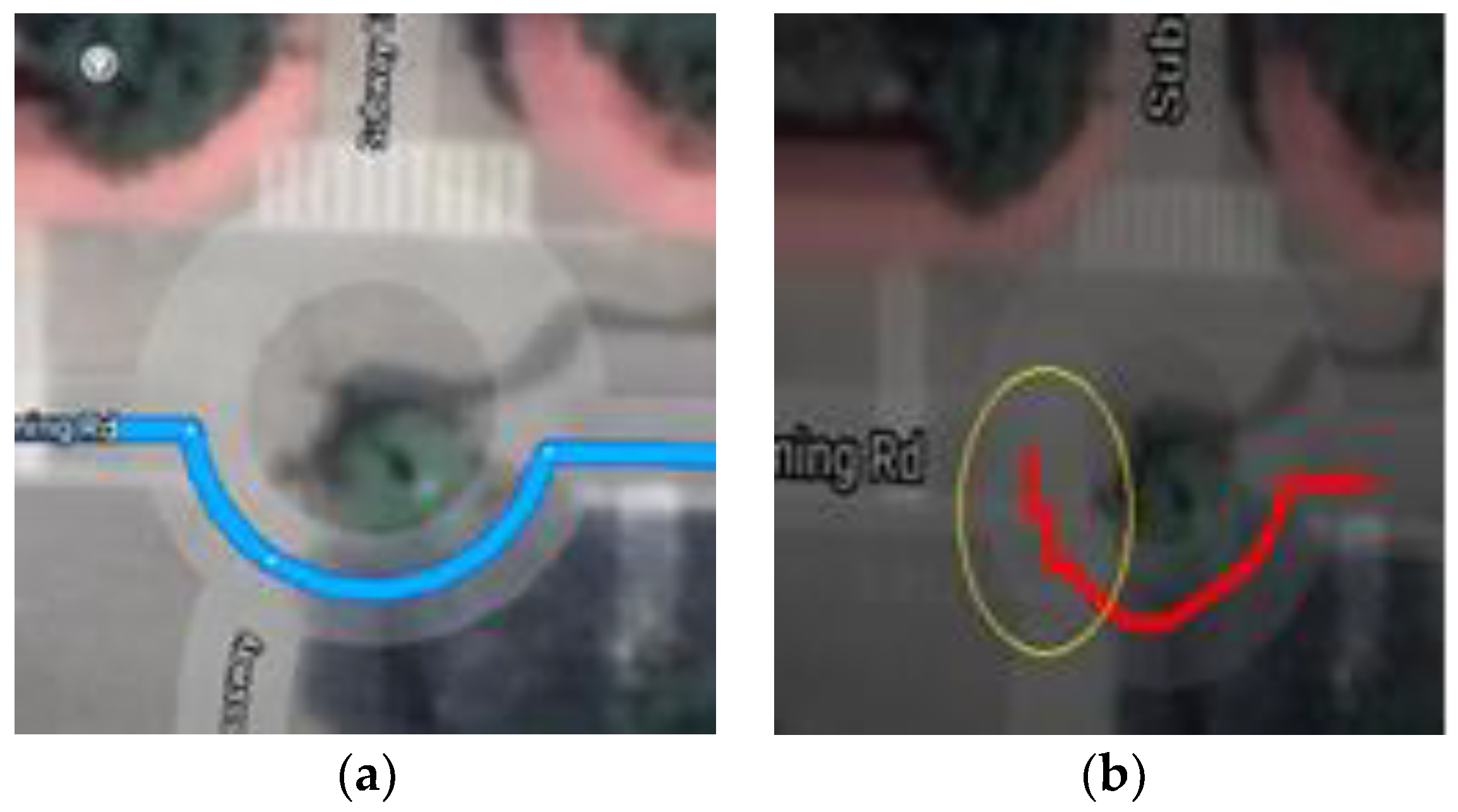
3.1. Proposed Curve Finding Method

The identified curve analysis is evaluated using the Type 1 error, Type 2 error, and Type 2 error ratio (TIIR) metrics [26]. When a Type 2 error occurs, an extra segment is added to the detected curve in comparison to the ground truth curve. Wherever a Type 1 error occurs, the detected curve is missing 25%, 50%, or 75% of the ground truth curve, or the curve is not identified. Figure 9a exhibits a 60% curve identification, while Figure 9b displays a distinct 50% curve identification, indicating that both are Type 1 errors. Figure 9c depicts Type 2 error because it inserts extra waypoints into curve waypoints, whereas the truth is that those waypoints should not be included in the curve. This type of Type 1 error is exceedingly harmful. Type 2 is not harmful, but the curve warning technique may warn the motorist that a curve exists. TIIR = m/n, where m is the number of Type 2 errors, n is the number of ground truth curves, and TIIR is the Type 2 error ratio.

Table 2. The study of proposed curve detection.

S.no	Origin & Destination	Total Distance of Path	Total No. of Curve Exist	Total No. of Curve Identified	Type 1 Error	Type 2 Error	Noise Corrected	TIIR	Total No. of Curve Identified by Reference [26]	Performance Delay (Milliseconds)	Performance Delay by Reference [27] (Milliseconds)
a	12.969096, 79.158385 & 12.968991, 79.158133	30 m	2	2	0	0	1	0.00	3	53	1245
b	12.968970, 79.158103 & 12.969291, 79.158617	200 m	3	3	0	1	1	0.33	4	355	8217
c	12.968467, 79.160714 & 12.969006, 79.161010	100 m	8	8	1 (25%)	4	10	0.5	18	177	4108

shows the total distance from the origin to destination, actual curve counts, identified curve counts, Type 1 error, Type 2 error, number of noise-adjusted curves in India’s campus sites, TIIR, identified curve counts by reference [26], proposed method performance delay in raspberry pi, and performance delay in raspberry pi by reference [27].

Row (a) examines the detection of indoor path curves. Row (b) is for on-road curve detection, while row (c) is for agricultural land curve detection. These three types of paths were created using the trajectory (path) creation methods described in Section 2.5. The indoor ground truth path is created by manually moving the AGV using a non-GPS location update. The path for on-road ground truth and agricultural land-based ground truth is based on hand-drawn lines over an open-street map. The proposed curve detection model finds curves in the path and eliminates noise on the curvature path. The existing curve identification approach, as illustrated in the tenth column of Table 2, is incapable of detecting this type of noise. The curve detection algorithm developed by Bil et al. [27] is capable of detecting path noise, but because this algorithm makes use of machine learning techniques, it uses more performance delay (Table 2 last column) when detecting curves. The proposed approach has a lower performance delay (Table 2 11th column) when detecting curves and noise. Many noises have been discovered and adjusted in row (c) because noise is generated in the path due to sliding and drifting in the dry agricultural land.

3.2. Metrics for Navigation Results

RMSE (Root Mean Square Error) is used to metrics of navigation errors.

$$RMSE=\sqrt{{\displaystyle \sum }_{i=1}^n\frac{{\left(g_i-p_i\right)}^2}{n}}$$

(13)

where $n$ denotes the number of events, $g_i$ denotes the ground truth, and $p_i$ denotes the predicted value. The ground truth $g_i$ is obtained using the trajectory (path) creation method described in Section 2.5. The path tracking algorithm generates the predicted value $p_i$. The number of events, $n$, is calculated from the number of units travelled by the AGV. The number of units here refers to the unit calculated by the Odometry Motion Model, as described in Section 2.2.

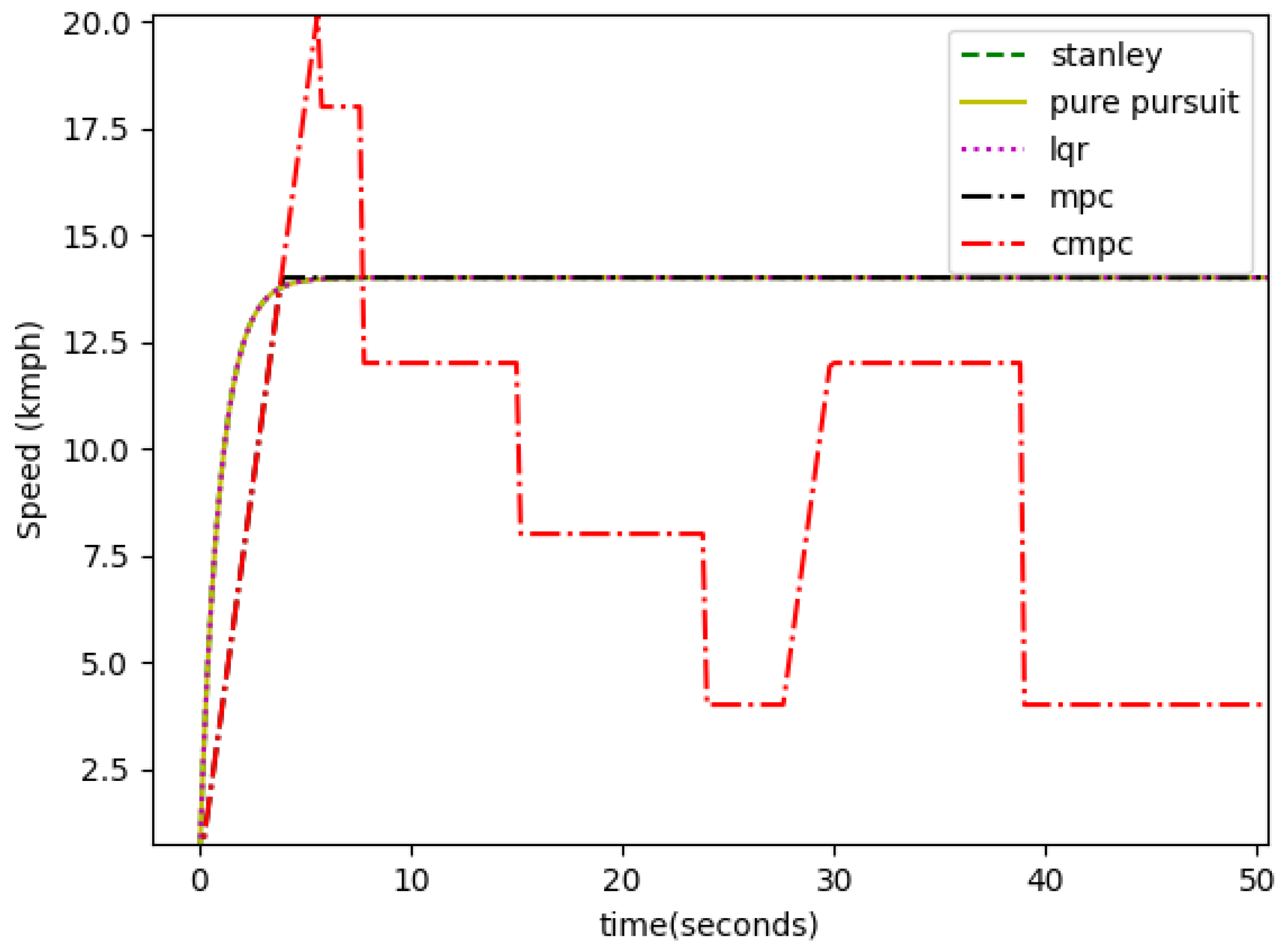
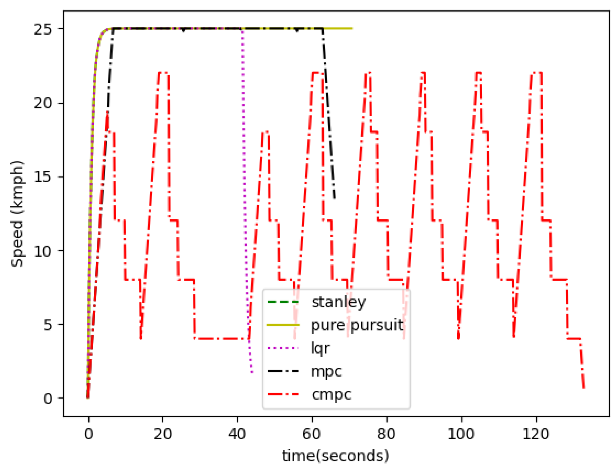
3.3. Curve-Aware MPC Result

Figure 10 and Figure 11 and

Table 3. The proposed C-MPC vs. MPC.

S.no	Mobile Robot Speed Set	Curve Speed Limit	RMSE of Lateral Error (m)		RMSE of Longitudinal Error (m)
			MPC	C-MPC	MPC	C-MPC
a	7 km/h	3 km/h	2.27	0.85	1.86	0.62
b	15 km/h	7 km/h	3.82	0.98	1.15	0.54
c	10 km/h	3 km/h	5.63	1.03	1.60	0.92

illustrate the real-time test-bed results comparing the existing MPC path tracking algorithm to the proposed C-MPC (curve-aware MPC). The three rows of curvature positions in Table 2 are entered into the test bed. The MPC and C-MPC have tested the Table 2 row (a) position indoor (Figure 10a and Figure 11a). Table 3 row (a) reveals that the AGV speed is set at 7 km/h and the in-door curve speed limit is 3 km/h; nevertheless, the MPC was unaware of the curve speed limit and traveled through the curve at 7 km/h, resulting in a large RMSE lateral and longitudinal error. The metrics RMSE were calculated by comparing the ground truth path to the AGV traveled path (Figure 11). The significant RMSE in lateral and longitudinal error indicates that the AGV’s traveled path, as managed by the MPC path tracking algorithm, has not gotten closer to the ground truth. The MPC has more longitudinal error (2.27 m) than lateral error (1.86 m), and the AGV driven by MPC was slightly dashed in the corridor wall, with more dash in the corridor turn wall, as shown in Figure 11a. C-MPC, on the other hand, was aware of the curve speed limit and slowed the AGV speed by 3 km/h before the curve (corridor turn) starting locations, allowing it to successfully go closer to the ground truth so that the C-MPC securely drove the AGV in the indoor environment with a lesser lateral error (0.85 m) and longitudinal (0.62 m) error. Figure 10a depicts an image of an indoor test bed.

Table 2 row (b) is tested in an on-road environment. In this scenario, the AGV steered by MPC was tested against the C-MPC. The AGV speed was set to 15 km/h in Table 3 row (b), while the curve speed limit was 7 km/h. In this test, the C-MPC navigated closer to the ground truth since it was aware of the curve and reduced AGV speed to 7 km/h, as well as achieving a lower RMSE in lateral (0.98 m) and longitudinal (0.54 m) error than the MPC. Due to the hand-drawn lines used to create the outdoor environment on-road trajectory in this case, the C-MPC lateral error is almost one meter. The hand-drawn curve is not made in the shape of an arch. However, the one-meter lateral error is due to the AGV turning in an arch shape. The MPC was set up with a constant speed of 15 km/h in an on-road environment, which caused the AGV to travel wider over curves and produce higher lateral (3.82 m) errors. Figure 11b clearly shows that the MPC-guided path was not closer to the ground truth. Figure 10b depicts an image of an on-road test bed.

The AGV encountered drift and sliding during testing on agricultural land (Table 2 row (c)), which is deemed noise on the path. The AGV speed was set at 10 km/h since it needed push power to travel on the dried agricultural land, but the curvature speed limit was 2 km/h, which implies the AGV had to turn slowly in the curve. The C-MPC achieved less lateral (1.03 m) and longitudinal (0.92 m) error than the MPC and moved much closer to the reference path (Figure 11c). However, the hand-drawn curvature trajectory ground truth caused the errors to be one meter. When the MPC was not moved closer to the ground truth due to curvature and was unaware of the curve speed limit, the AGV jolted and went wide against the ground truth, resulting in a higher lateral error (5.63 m). Figure 10c depicts a view of an agricultural land testbed.

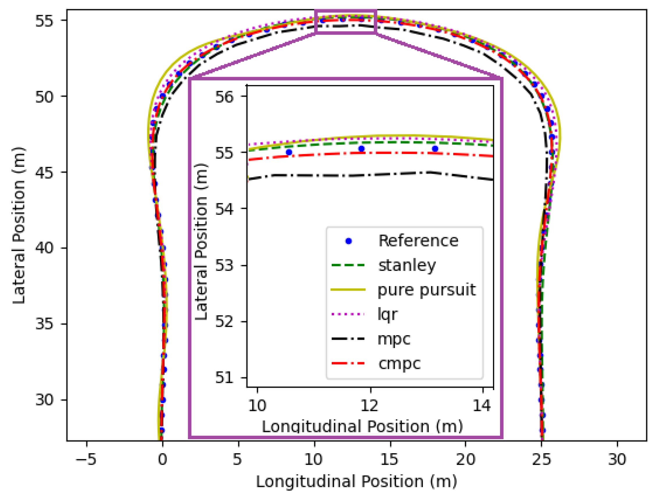
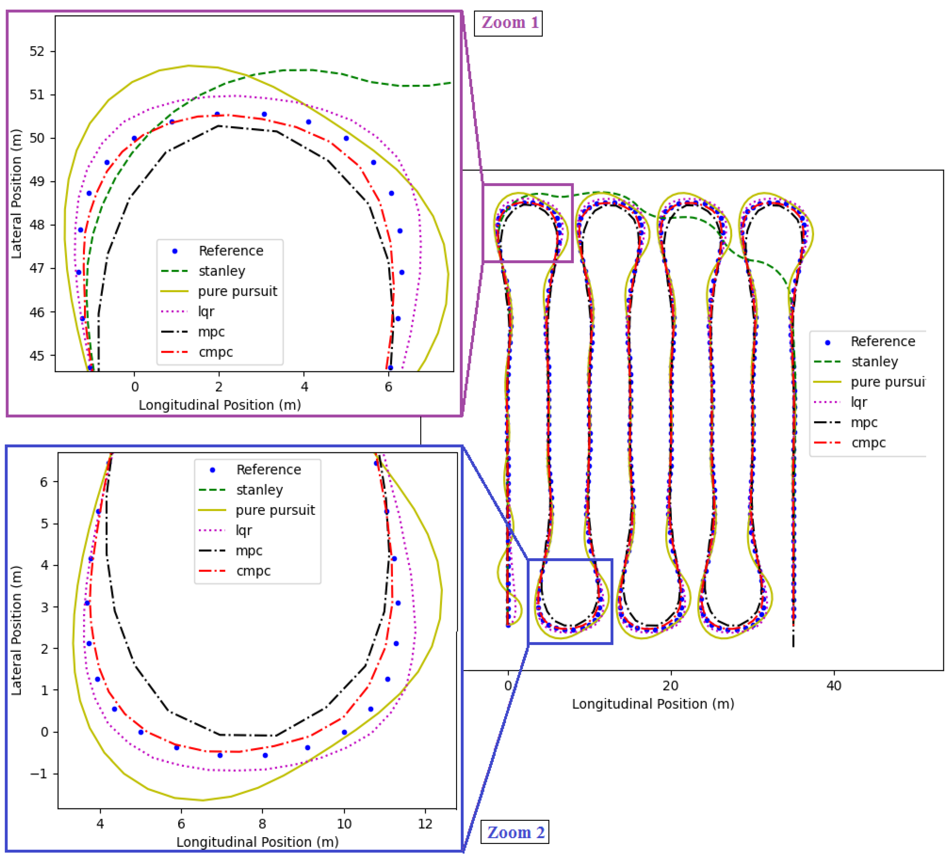
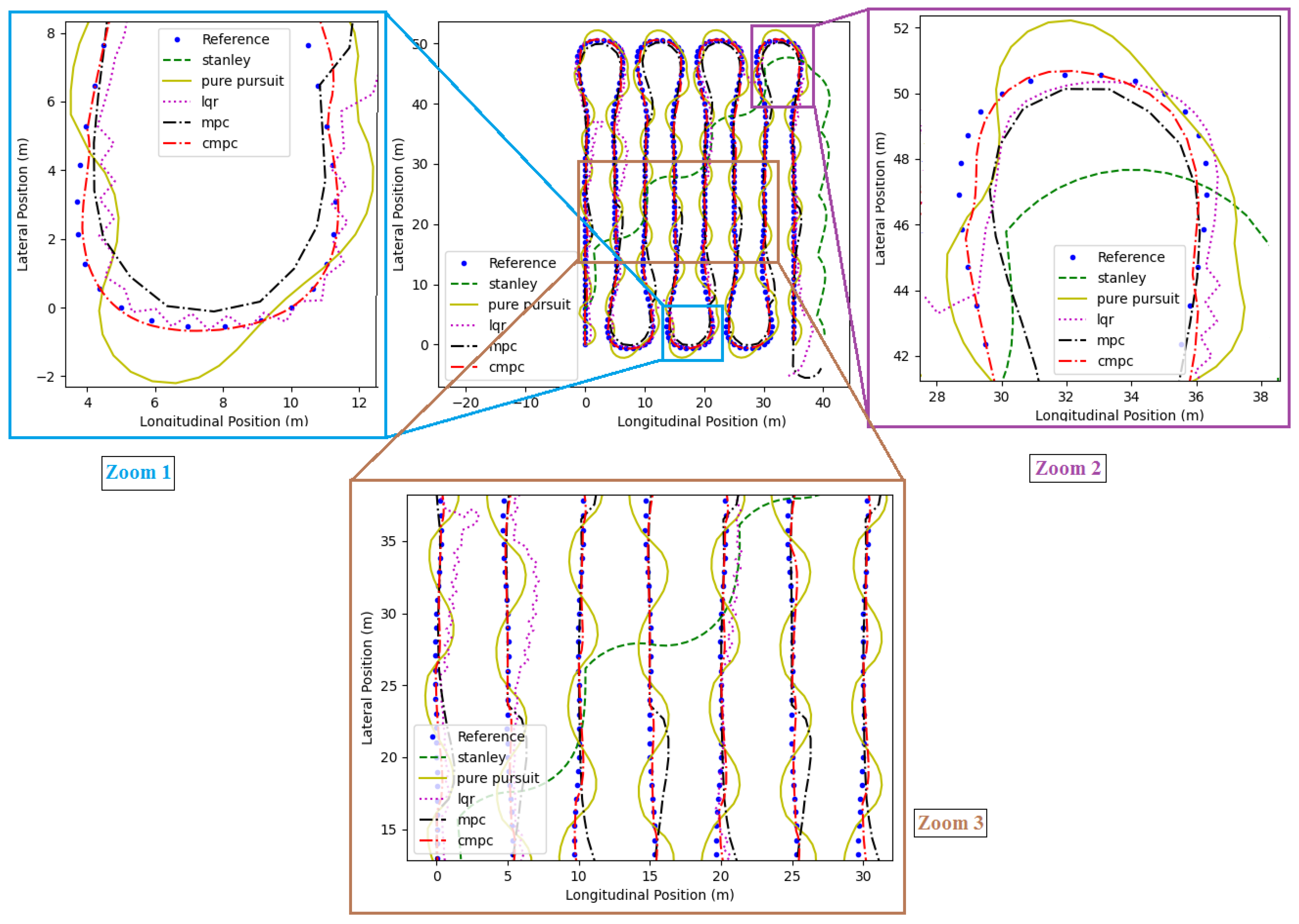
3.4. Simulation Setup and Results

Only the MPC and C-MPC have been tested in real-time. Various existing path-tracking algorithms can guide the AGV along the path. As a result, simulation was used to test both the present path tracking method and the proposed C-MPC. PythonRobotics [37], a python-based program, was utilized for simulation. This tool creates the road geometry as well as simulates AGV movement along the path. Four existing path-tracking algorithms can be used to traverse the simulated AGV, and they are compared to the proposed C-MPC. Path tracking algorithms that are now in use include pure pursuit, Stanley, Linear Quadratic Regulator (LQR), and Model Predictive Control (MPC). The results are compared to the root mean square error (RMSE) of lateral and longitudinal error, speed vs. time, and moving trajectory. The simulation test-bed has three scenarios: indoor navigation, on-road navigation, and agricultural navigation.

• Test-bed 1:

During the indoor simulation, the path geometry was built with four straight lines and three turns, as illustrated in Figure 12. The simulated AGV’s speed was set at 15 km/h. In this indoor environment, the existing path tracking algorithm and the proposed C-MPC were tested.

Table 4. The proposed model vs. the existing trajectory tracking model over indoor.

S.no	Path Tracking Algorithms	RMSE of Lateral Error (m)	RMSE of Longitudinal Error (m)
1	Pure Pursuit	0.22	0.37
2	Stanley	1.98	4.57
3	LQR	0.07	0.10
4	MPC	1.49	0.41
5	Proposed C-MPC	0.12	0.30

lists the RMSE errors, and Figure 13 depicts the speed vs. time result.

The speed of the simulated AGV navigated by existing path tracking algorithms is constant at 15 km/h along the path, while the C-MPC with curve aware speed limit navigates the simulated AGV in the curvature area at the curve limit speed, as illustrated in Figure 13 (red line). When the simulated AGV that is being navigated by C-MPC, approaches a curve, the C-MPC reduces the simulated AGV’s constant speed from 15 km/h to 7 km/h and navigates the simulated AGV over the curve. As shown in Figure 13 (red line), from the 7th to the 25th second, the simulated AGV speed was gradually reduced and traveled with a curvature-restricted speed limit; once it traveled the curvature, the speed increased to the setup speed of 15 km/h. When another curve is approached, the simulated AGV speed is reduced to the speed limit of the next curve.

Figure 12 depicts the trajectory tracking footprint of each algorithm as well as the reference path. Based on a constant speed of 15 km/h, the Stanley maneuvered the simulated AGV away from the reference path (ground truth). In this case, the simulated AGV was steered by pure pursuit more nearly to the reference path during the straight line, resulting in a reduced error in RMSE lateral (0.22 m) and longitudinal (0.37 m) error.

However, the Stanley was unable to navigate closer to the reference path in a straight line because of the constant speed of the simulated AGV, resulting in a significant RMSE lateral (1.98 m) and longitudinal (4.97 m) error. Here, the LQR, MPC, and C-MPC are navigated closer to the reference path. The C-MPC navigated significantly closer than other path-tracking algorithms (Figure 12 zoom 1), while the LQR performed better in the third curve (Figure 12 zoom 2). The third curve is of the reverse type (‘S’), so all path tracking algorithms except LQR moved wider. Furthermore, while the LQR had the lowest RMSE lateral (0.07 m) and longitudinal (0.10 m) error, the C-MPC lateral (0.12 m) and longitudinal (0.30 m) error did not differ significantly from the LQR error. The MPC navigated the simulated AGV wider of the curvature path due to constant speed, and it obtained a higher lateral (1.49 m) error.

• Test-bed 2:

Figure 14 depicts the intended path geometry for on-road testing simulation, which includes two straight lines and one curvature. The simulated AGV’s speed has been set at 25 km/h. In this on-road scenario, the existing path tracking algorithm and the proposed C-MPC have been tested.

Table 5. The proposed model vs. the existing trajectory tracking model over on-road.

S.no	Path Tracking Algorithms	RMSE of Lateral Error (m)	RMSE of Longitudinal Error (m)
1	Pure Pursuit	0.23	0.37
2	Stanley	0.84	1.26
3	LQR	0.15	0.37
4	MPC	0.32	2.78
5	Proposed C-MPC	0.06	0.36

lists the RMSE errors, and Figure 15 depicts the speed vs. time result.

The speed of the simulated AGV navigated by existing path tracking algorithms is constant at 25 km/h along the path, while the C-MPC with a curve aware speed limit navigates the simulated AGV in the curvature area at the curve limit speed, as illustrated in Figure 15 (red line). However, the proposed C-MPC took 50 s to complete the path, whilst others finished in less than 25 s. Because the C-MPC navigated the AGV in the curvature path at a lower speed of 8 km/h, the C-MPC first drives the AGV at 20 km/h before reaching the curvature in the curve alert point, and the AGV speed gradually decreased. As a result, the C-MPC method pushes the simulated AGV substantially closer to the reference path and has lower RMSE lateral (0.06 m) and longitudinal (0.36 m) errors than the existing algorithm. The longitudinal errors for the Stanley (1.26 m) and MPC (2.78 m) were higher because both algorithms navigated the simulated AGV inside the curve.

• Test-bed 3:

The intended path shape in the Agricultural land testing simulation contains eight straight lines and seven curves, as shown in Figure 16. The simulated AGV’s speed has been set at 25 km/h. In this agricultural field scenario, the existing path tracking algorithm and the proposed C-MPC have been tested.

Table 6. The proposed model vs. the existing trajectory tracking model over agricultural land.

S.no	Path Tracking Algorithms	RMSE of Lateral Error (m)	RMSE of Longitudinal Error (m)
1	Pure Pursuit	0.21	0.81
2	Stanley (failed)	1.37	4.01
3	LQR	0.08	0.73
4	MPC	0.30	1.80
5	Proposed C-MPC	0.07	0.62

lists the RMSE errors, and Figure 17 depicts the speed vs. time result.

The speed of the simulated AGV navigated by existing path tracking algorithms is constant at 25 km/h along the path, while the C-MPC with curve aware speed limit navigates the simulated AGV in the curvature area at the curve limit speed, as illustrated in Figure 17 (red line). However, the proposed C-MPC took 120 s to complete the path, whilst others finished in less than 65 s. Because the C-MPC drove the simulated AGV in the curvature path at a reduced speed of 8 km/h to 4 km/h, the C-MPC first drives the simulated AGV at 22 km/h before reaching the curvature in the curve alert site; the AGV speed has gradually decreased.

As a result, the C-MPC method pushes the simulated AGV substantially closer to the reference path and has lower RMSE lateral (0.07 m) and longitudinal (0.62 m) errors than the present approach. The Stanley algorithm emerged from the path depicted in Figure 16 (green dash line). When the simulated AGV is navigated by the MPC inside the curve (Figure 16 zoom 1 and zoom 2), the longitudinal error was higher (1.80 m).

• Test-bed 4:

The chosen path shape in agricultural land with sliding error testing simulation contains eight straight lines and seven curves, as illustrated in Figure 18. The simulated AGV’s speed has been set at 25 km/h. In this agricultural field scenario, the existing path tracking algorithm and the proposed C-MPC have been tested.

Table 7. The proposed model vs. the existing trajectory tracking model over agricultural land with sliding.

S.no	Path Tracking Algorithms	RMSE of Lateral Error (m)	RMSE of Longitudinal Error (m)
1	Pure Pursuit	1.76	1.82
2	Stanley (failed)	11.71	3.44
3	LQR	0.84	1.51
4	MPC	0.71	2.77
5	Proposed C-MPC	0.09	0.69

lists the RMSE errors, and Figure 19 depicts the speed vs. time result.

The sliding error model was simulated in this test-bed using Equations (8)–(10), as mentioned in the Noise Model for Odometry section. There are 46 sliding noises simulated, with four noises in each straight line and two noises in each curve. The Stanley and LQR failed on path tracking because of too fast speed and sliding noise, which is seen in Figure 18 zoom 3 and in Figure 19, both of which finished in less than 45 s. In comparison to the pure pursuit, LQR and MPC, the proposed C-MPC navigated the simulated AGV on the reference path, while also managing sliding noise, as shown in Figure 18 zoom 1 to 3. Because it was aware of the curve speed limit, the C-MPC successfully steered the simulated AGV through the curvature, as shown in Figure 20. As a result, it has a much lower RMSE lateral (0.09 m) and longitudinal (0.69 m) error than other existing algorithms. The Stanley algorithm emerged from the path depicted in Figure 16 zoom 3 (green dash line). Both LQR and MPC had higher longitudinal errors (LQR: 1.51 m & MPC: 2.77 m) when navigating the simulated AGV inside the curve. In terms of lateral (1.76 m) and longitudinal (1.82 m) RMSE error, the pure pursuit path tracking algorithm is worse.

4. Discussion

Table 8. Comparative study of the proposed model with existing models.

S.no	Methods	Navigation Type	Purpose	Curvature Method	Cost of Navigation
1	Ref. [19]	Vision	on-Road navigation	Image processing-based road edge features are extracted and calculated for a curvature or straight line. AGV moves at a constant speed.	High (embedded board and camera, 3D laser beam is high cost) [19,20,22]
2	Ref. [16]	Tape and vision	In-door navigation	Image processing-based tape features are extracted and calculated for a curvature or straight line. AGV moves at a constant speed.	Moderate (depends on embedded board, camera, and amount of floor fixing tape required) [20,22]
3	Ref. [23]	Vision	Agricultural navigation	Image processing-based crop row features are extracted and calculated for a curvature or straight line. AGV moves at a constant speed.	Moderate (depends on embedded board, camera, and other sensors cost) [20,22]
4	Proposed model	Google map data	on-Road, In-door, and Agricultural navigation	The proposed curve finding method extracts the curve from generated trajectory (path) and reduces mobile robot speed before reaching the curve starting point. AGV moves at variable speed.	Low (using low-cost embedded board) [22]

compares the proposed method with existing methods in terms of navigation type, purpose, curvature method, and system cost. According to J.H. Han et al. [19], a web camera installed on the AGV was used to extract road features, and the AGV successfully traveled, as shown in Figure 21a,b. The test is conducted on a bright and sunny day. However, the AGV struggled to travel in the junction site shown in Figure 21c,d since the area is wider and the road boundaries are difficult to find. This problem may be avoided if the AGV was bigger.

The AGV successfully traveled in the required tape-type path (Figure 22a,b) with constant speed when tested in an indoor area using the D. Puppim de Oliveira et al. [16] approach. When the AGV speed increased from 0.08 m/s to 0.29 m/s [10], the AGV breaks from the tape-type path (Figure 22c,d) as it approaches curvature.

J. Bengochea-Guevara et al. [23] successfully navigated and maneuvered across the row change in constant speed in agricultural terrain testing. When the AGV’s speed increased, the AGV exited the path in a row and changed the curvature location, as shown in Figure 23b.

In comparison to all existing methods, the proposed C-MPC successfully navigates the AGV in indoor, on-road, and agricultural terrain; with curvature awareness, the AGV navigated by the C-MPC moves at variable speed. The proposed navigation system is inexpensive because it runs on a Raspberry Pi device. In terms of environmental sustainability, one can calculate the carbon emissions (CO₂) of this processing unit using a green algorithm [38,39] calculator for Green Computing. The raspberry pi emits 0.040 kg of CO₂ per day, making it the lowest carbon-emitting device and hence acceptable for environmental sustainability.

The proposed C-MPC algorithm navigates the AGV using IMU and Hall Effect sensors. It has limitations when it deviates from its reference path and is violently dashed by any object. Future research on the issue will make use of decision-making approaches, such as the scheduling algorithm [40,41,42] and metaheuristic algorithm [43,44,45,46]. In addition, the AGV will include additional sensors, such as obstacle detection, to help it to navigate over the obstacle.

5. Conclusions

Curvature can be found in paths that are established indoors, on the road, or on agricultural land. Automatically driving the AGV through the curve path is more difficult due to the AGV’s constant speed. The AGV needs to start from the indoor (the shed) and go on the road to reach agricultural terrain, where it must then perform agricultural navigation. A single path tracking algorithm is required for all terrain navigation. In all terrains, the proposed curve-aware MPC (C-MPC) extracts the curve from the Google map path, and the proposed curve-aware MPC (C-MPC) successfully navigates the AGV. The proposed method guided the AGV successfully with lower RMSE lateral and longitudinal error, according to real-time and simulation results. The proposed method’s limitations, such as obstacle overtaking and sudden course-altering error, will be studied using decision-making approaches in future research. The proposed C-MPC approach is now being tested in a campus-like environment and will afterward be applied in an industry-like environment.

References

1. Motroni, A.; Buffi, A.; Nepa, P. Forklift Tracking: Industry 4.0 Implementation in Large-Scale Warehouses through UWB Sensor Fusion. Appl. Sci. 2021, 11, 10607. [Google Scholar] [CrossRef]
2. Stetter, R. A Fuzzy Virtual Actuator for Automated Guided Vehicles. Sensors 2020, 20, 4154. [Google Scholar] [CrossRef] [PubMed]
3. Teso-Fz-Betoño, D.; Zulueta, E.; Fernandez-Gamiz, U.; Aramendia, I.; Uriarte, I. A Free Navigation of an AGV to a Non-Static Target with Obstacle Avoidance. Electronics 2019, 8, 159. [Google Scholar] [CrossRef]
4. Ito, S.; Hiratsuka, S.; Ohta, M.; Matsubara, H.; Ogawa, M. Small Imaging Depth LIDAR and DCNN-Based Localization for Automated Guided Vehicle. Sensors 2018, 18, 177. [Google Scholar] [CrossRef]
5. Saputra, R.P.; Rijanto, E. Automatic Guided Vehicles System and Its Coordination Control for Containers Terminal Logistics Application. arXiv 2021, arXiv:2104.08331. [Google Scholar]
6. Gonzalez-de-Santos, P.; Fernández, R.; Sepúlveda, D.; Navas, E.; Emmi, L.; Armada, M. Field Robots for Intelligent Farms—Inhering Features from Industry. Agronomy 2020, 10, 1638. [Google Scholar] [CrossRef]
7. Gu, Y.; Li, Z.; Zhang, Z.; Li, J.; Chen, L. Path Tracking Control of Field Information-Collecting Robot Based on Improved Convolutional Neural Network Algorithm. Sensors 2020, 20, 797. [Google Scholar] [CrossRef] [PubMed]
8. Gul, F.; Rahiman, W.; Nazli Alhady, S.S. A Comprehensive Study for Robot Navigation Techniques. Cogent Eng. 2019, 6, 1632046. [Google Scholar] [CrossRef]
9. Moshayedi, A.J.; Jinsong, L.; Liao, L. AGV (automated guided vehicle) robot: Mission and obstacles in design and performance. J. Simul. Anal. Nov. Technol. Mech. Eng. 2019, 12, 5–18. [Google Scholar]
10. Bechtel, M.G.; Mcellhiney, E.; Kim, M.; Yun, H. DeepPicar: A Low-Cost Deep Neural Network-Based Autonomous Car. In Proceedings of the 2018 IEEE 24th International Conference on Embedded and Real-Time Computing Systems and Applications (RTCSA), Hokkaido, Japan, 28–31 August 2018. [Google Scholar]
11. Wang, S.; Chen, X.; Ding, G.; Li, Y.; Xu, W.; Zhao, Q.; Gong, Y.; Song, Q. A Lightweight Localization Strategy for LiDAR-Guided Autonomous Robots with Artificial Landmarks. Sensors 2021, 21, 4479. [Google Scholar] [CrossRef]
12. Zhang, S.; Wang, Y.; Zhu, Z.; Li, Z.; Du, Y.; Mao, E. Tractor Path Tracking Control Based on Binocular Vision. Inf. Process. Agric. 2018, 5, 422–432. [Google Scholar] [CrossRef]
13. Akhshirsh, G.S.; Al-Salihi, N.K.; Hamid, O.H. A Cost-Effective GPS-Aided Autonomous Guided Vehicle for Global Path Planning. Bull. Electr. Eng. Inform. 2021, 10, 650–657. [Google Scholar] [CrossRef]
14. Hodson, T.O. Root-mean-square error (RMSE) or mean absolute error (MAE): When to use them or not. Geosci. Model Dev. 2022, 15, 5481–5487. [Google Scholar] [CrossRef]
15. Aghi, D.; Cerrato, S.; Mazzia, V.; Chiaberge, M. Deep Semantic Segmentation at the Edge for Autonomous Navigation in Vineyard Rows. In Proceedings of the 2021 IEEE/RSJ International Conference on Intelligent Robots and Systems (IROS), Prague, Czech Republic, 27 September–1 October 2021. [Google Scholar] [CrossRef]
16. Puppim de Oliveira, D.; Pereira Neves Dos Reis, W.; Morandin Junior, O. A Qualitative Analysis of a USB Camera for AGV Control. Sensors 2019, 19, 4111. [Google Scholar] [CrossRef] [PubMed]
17. Nguyen, P.T.-T.; Yan, S.-W.; Liao, J.-F.; Kuo, C.-H. Autonomous Mobile Robot Navigation in Sparse LiDAR Feature Environments. Appl. Sci. 2021, 11, 5963. [Google Scholar] [CrossRef]
18. Wu, X.; Sun, C.; Zou, T.; Xiao, H.; Wang, L.; Zhai, J. Intelligent Path Recognition against Image Noises for Vision Guidance of Automated Guided Vehicles in a Complex Workspace. Appl. Sci. 2019, 9, 4108. [Google Scholar] [CrossRef]
19. Han, J.-H.; Kim, H.-W. Lane Detection Algorithm Using LRF for Autonomous Navigation of Mobile Robot. Appl. Sci. 2021, 11, 6229. [Google Scholar] [CrossRef]
20. Bi, S.; Yuan, C.; Liu, C.; Cheng, J.; Wang, W.; Cai, Y. A Survey of Low-Cost 3D Laser Scanning Technology. Appl. Sci. 2021, 11, 3938. [Google Scholar] [CrossRef]
21. Medina Sánchez, C.; Zella, M.; Capitán, J.; Marrón, P.J. From Perception to Navigation in Environments with Persons: An Indoor Evaluation of the State of the Art. Sensors 2022, 22, 1191. [Google Scholar] [CrossRef]
22. Suzen, A.A.; Duman, B.; Sen, B. Benchmark Analysis of Jetson TX2, Jetson Nano and Raspberry PI Using Deep-CNN. In Proceedings of the 2020 International Congress on Human-Computer Interaction, Optimization and Robotic Applications (HORA), Ankara, Turkey, 26–28 June 2020. [Google Scholar] [CrossRef]
23. Bengochea-Guevara, J.M.; Conesa-Muñoz, J.; Andújar, D.; Ribeiro, A. Merge Fuzzy Visual Servoing and GPS-Based Planning to Obtain a Proper Navigation Behavior for a Small Crop-Inspection Robot. Sensors 2016, 16, 276. [Google Scholar] [CrossRef]
24. Liu, Z.; Zheng, W.; Wang, N.; Lyu, Z.; Zhang, W. Trajectory Tracking Control of Agricultural Vehicles Based on Disturbance Test. Int. J. Agric. Biol. Eng. 2020, 13, 138–145. [Google Scholar] [CrossRef]
25. Han, J.-H.; Park, C.-H.; Kwon, J.H.; Lee, J.; Kim, T.S.; Jang, Y.Y. Performance Evaluation of Autonomous Driving Control Algorithm for a Crawler-Type Agricultural Vehicle Based on Low-Cost Multi-Sensor Fusion Positioning. Appl. Sci. 2020, 10, 4667. [Google Scholar] [CrossRef]
26. Li, Z.; Chitturi, M.V.; Bill, A.R.; Noyce, D.A. Automated Identification and Extraction of Horizontal Curve Information from Geographic Information System Roadway Maps. Transp. Res. Rec. 2012, 2291, 80–92. [Google Scholar] [CrossRef]
27. Bíl, M.; Andrášik, R.; Sedoník, J.; Cícha, V. ROCA-An ArcGIS toolbox for road alignment identification and horizontal curve radii computation. PLoS ONE 2018, 13, e0208407. [Google Scholar] [CrossRef]
28. Ge, J.; Pei, H.; Yao, D.; Zhang, Y. A Robust Path Tracking Algorithm for Connected and Automated Vehicles under I-VICS. Transp. Res. Interdiscip. Perspect. 2021, 9, 100314. [Google Scholar] [CrossRef]
29. Wang, L.; Zhai, Z.; Zhu, Z.; Mao, E. Path Tracking Control of an Autonomous Tractor Using Improved Stanley Controller Optimized with Multiple-Population Genetic Algorithm. Actuators 2022, 11, 22. [Google Scholar] [CrossRef]
30. Yang, T.; Bai, Z.; Li, Z.; Feng, N.; Chen, L. Intelligent Vehicle Lateral Control Method Based on Feedforward + Predictive LQR Algorithm. Actuators 2021, 10, 228. [Google Scholar] [CrossRef]
31. Chen, J.; Shi, Y. Stochastic Model Predictive Control Framework for Resilient Cyber-Physical Systems: Review and Perspectives. Philos. Trans. A Math. Phys. Eng. Sci. 2021, 379, 20200371. [Google Scholar] [CrossRef]
32. Huang, Z.; Li, H.; Li, W.; Liu, J.; Huang, C.; Yang, Z.; Fang, W. A New Trajectory Tracking Algorithm for Autonomous Vehicles Based on Model Predictive Control. Sensors 2021, 21, 7165. [Google Scholar] [CrossRef]
33. Jeong, Y.; Yim, S. Model Predictive Control-Based Integrated Path Tracking and Velocity Control for Autonomous Vehicle with Four-Wheel Independent Steering and Driving. Electronics 2021, 10, 2812. [Google Scholar] [CrossRef]
34. Thrun, S.; Burgard, W.; Fox, D. Probabilistic Robotics; MIT Press: London, UK, 2005; ISBN 9780262201629. [Google Scholar]
35. IRC:73-1980; Geometric Design Standards for Rural (Non-Urban) Highways. Indian Roads Congress: New Delhi, India, 1990.
36. IRC:38-1988; Guidelines for Design of Horizontal Curves for Highways and Design Tables. Indian Roads Congress: New Delhi, India, 1989.
37. Available online: https://github.com/AtsushiSakai/PythonRobotics (accessed on 17 December 2021).
38. Lannelongue, L.; Grealey, J.; Inouye, M. Green Algorithms: Quantifying the Carbon Footprint of Computation. Adv. Sci. 2021, 8, 2100707. [Google Scholar] [CrossRef] [PubMed]
39. Dev, K.; Xiao, Y.; Gadekallu, T.R.; Corchado, J.M.; Han, G.; Magarini, M. Guest Editorial Special Issue on Green Communication and Networking for Connected and Autonomous Vehicles. IEEE Trans. Green Commun. Netw. 2022, 6, 1260–1266. [Google Scholar] [CrossRef]
40. Dulebenets, M. A diploid evolutionary algorithm for sustainable truck scheduling at a cross-docking facility. Sustainability 2018, 10, 1333. [Google Scholar] [CrossRef]
41. Kavoosi, M.; Dulebenets, M.A.; Abioye, O.F.; Pasha, J.; Wang, H.; Chi, H. An augmented self-adaptive parameter control in evolutionary computation: A case study for the berth scheduling problem. Adv. Eng. Inform. 2019, 42, 100972. [Google Scholar] [CrossRef]
42. Dulebenets, M.A. An Adaptive Polyploid Memetic Algorithm for scheduling trucks at a cross-docking terminal. Inf. Sci. 2021, 565, 390–421. [Google Scholar] [CrossRef]
43. Pasha, J.; Nwodu, A.L.; Fathollahi-Fard, A.M.; Tian, G.; Li, Z.; Wang, H.; Dulebenets, M.A. Exact and metaheuristic algorithms for the vehicle routing problem with a factory-in-a-box in multi-objective settings. Adv. Eng. Inform. 2022, 52, 101623. [Google Scholar] [CrossRef]
44. Tripathy, B.K.; Reddy Maddikunta, P.K.; Pham, Q.V.; Gadekallu, T.R.; Dev, K.; Pandya, S.; ElHalawany, B.M. Harris Hawk Optimization: A Survey onVariants and Applications. Comput. Intell. Neurosci. 2022, 2022, 2218594. [Google Scholar] [CrossRef]
45. Ravi, C.; Tigga, A.; Reddy, G.T.; Hakak, S.; Alazab, M. Driver Identification Using Optimized Deep Learning Model in Smart Transportation. ACM Trans. Internet Technol. 2020. [Google Scholar] [CrossRef]
46. Hakak, S.; Gadekallu, T.R.; Ramu, S.P.; Maddikunta, P.K.R.; de Alwis, C.; Liyanage, M. Autonomous Vehicles in 5G and Beyond: A Survey. arXiv 2022, arXiv:2207.10510. [Google Scholar]
Figure 1. Testing scenario.
Sustainability 14 12021 g001
Figure 2. Proposed model block diagram.
Sustainability 14 12021 g002
Figure 3. Proposed AGV.
Sustainability 14 12021 g003
Figure 4. AGV steering angle.
Sustainability 14 12021 g004
Figure 5. Odometry motion model.
Sustainability 14 12021 g005
Figure 6. (a) Google map road segment points (b) Found curve.
Sustainability 14 12021 g006
Figure 7. (a) Noise in the curve (b) Eliminated noise in the curve.
Sustainability 14 12021 g007
Figure 8. Proposed curve-aware MPC timeline.
Sustainability 14 12021 g008
Figure 9. (a) and (b) different 50% curve identification of Type 1 error (c) Type 2 error.
Sustainability 14 12021 g009
Figure 10. AGV in testing (a) In-door test (b) On-road test (c) Agricultural land test.
Sustainability 14 12021 g010
Figure 11. AGV trajectory (a) In-door test (b) On-road test (c) Agricultural land test.
Sustainability 14 12021 g011
Figure 12. Indoor trajectory tracking footprint.
Sustainability 14 12021 g012
Figure 13. Time vs. speed in indoor navigation.
Sustainability 14 12021 g013
Figure 14. On-road trajectory tracking footprint.
Sustainability 14 12021 g014
Figure 15. Time vs. speed in on-road navigation.
Sustainability 14 12021 g015
Figure 16. Agricultural trajectory tracking footprint.
Sustainability 14 12021 g016
Figure 17. Time vs. speed in agricultural land navigation.
Sustainability 14 12021 g017
Figure 18. Agricultural land with sliding error trajectory tracking footprint.
Sustainability 14 12021 g018
Figure 19. Time vs. speed in agricultural land with sliding navigation.
Sustainability 14 12021 g019
Figure 20. Speed management by C-MPC over curvature.
Sustainability 14 12021 g020
Figure 21. On-road vision-based algorithm results in (a) Road edge detection (b) Obstacle on the road (c) Google map road junction image (d) mobile robot vision result in the road junction.
Sustainability 14 12021 g021
Figure 22. Indoor vision-based algorithm result (a) tape on the floor (b) existing model result (c) tape on floor curvature (d) curvature result.
Sustainability 14 12021 g022
Figure 23. Agricultural vision-based algorithm result (a) Edge of agricultural path making (b) Struggled in curvature.
Sustainability 14 12021 g023