Terminal Cooling Load Forecasting Model Based on Particle Swarm Optimization

Abstract

With the development of the civil aviation industry, the passenger throughput of airports has increased explosively, and they need to carry a large number of passengers every day and maintain operations for a long time. These factors cause the large space buildings in the airport to have higher energy consumption than ordinary buildings and have energy-saving potential. In practical engineering, there are problems such as low accuracy of prediction results due to inability to provide accurate building parameters and design parameters, some scholars oversimplify the large space building load forecasting model, and the prediction results have no reference significance. Therefore, establishing a load forecasting model that is closer to the actual operating characteristics and laws of large space buildings has become a research difficulty. This paper analyzes and compares the building and load characteristics of airport large space buildings, which are different from general large space buildings. The factors influencing large space architecture are divided into time characteristics and space characteristics, and the influencing reasons and characteristics of each factor are discussed. The Pearson analysis method is used to eliminate the influence parameters that have a very low connection with the cooling load, and then the historical data that affect the cooling load parameters are input. The MATLAB software is used to select a variety of neural network models for training and prediction. On this basis, the particle swarm optimization algorithm is used to optimize the prediction model. The results show that the prediction effect of the gated recurrent neural network based on particle swarm optimization algorithm is the best, the average absolute percentage error is only 0.7%, and the prediction accuracy is high.

1. Introduction

An airport is regarded as a small city with a complex energy system. Compared with traditional civil buildings, an airport terminal is characterized by a large space surrounded by a large area of glass curtain walls. It needs to accommodate a large number of passengers every day and maintain operation for a long time. All these factors will lead to higher air conditioning energy consumption. Many existing studies have pointed out that the energy use intensity at the airport terminal is higher than that of other common civil buildings, in which the heating, ventilation and air conditioning systems account for the largest share (40–80%) [1].

Starting from the source, the airport large space load has the problems of many disturbance factors and uneven load space–time distribution. In addition, the airport large space buildings operate all year round and the inner area has long-term cooling. In order to facilitate prediction, some scholars use regression analysis to simplify the model. Wei [2] et al. used the regression analysis method to regress the unknown parameters in the model in combination with the cooling load heat transfer formula and used historical data to test the model. Tang [3] et al. judged the existing data in a mathematical way to predict the load at a certain time in the future. The data set is required to be linear and stable. The prediction error on the non-stationary nonlinear data is too large, but the real prediction environment usually has strong volatility. The regression analysis method has a simple algorithm and can obtain good prediction results for regular data. However, due to the linear relationship between influencing factors, the accuracy of the regression model is reduced [4] and has no practical reference significance. Therefore, an accurate airport load forecasting model has become the key to energy conservation of large space buildings.

Common artificial intelligence methods mainly include artificial neural network (ANN), long time series memory network (LSTM), gated recurrent neural network (GRU), etc. The neural network forecasting method is more suitable for building load forecasting [5]. Recurrent neural networks (RNNs) are usually trained using back propagation through time or real-time recursive learning algorithms. Because the gradient disappears, the training using these methods usually fails. Different from the RNN model, the LSTM model can solve the gradient problem existing in RNN at different stages, but the calculation is large and time-consuming. Ren [6] and others compared the arimax model and LSTM model to predict airport passenger flow, and the results showed that the latter had high prediction accuracy. Zheng [7] et al. proposed a short-term load forecasting method of multi-layer long- and short-term memory neural network (ML-LSTM) considering temperature fuzziness. The LSTM was optimized by the Adam algorithm, which improved the forecasting accuracy and generalization of the proposed model. Xie [8] et al. predicted the heat load of the heating system of the airport terminal and proposed the GRU neural network prediction model based on the variable mode decomposition with high accuracy. Gong [9] et al. used the particle swarm optimization algorithm to optimize the GRU model. The results show that the model prediction effect is better after algorithm optimization. Tang [10] et al. proposed a multilayer bidirectional recurrent neural network model based on LSTM and GRU to predict short-term power load and compared it with LSTM, support vector regression, and back propagation models. The results show that the prediction accuracy of LSTM and GRU models proposed by the author is higher. Zhao [11] and others proposed the CNN-GRU short-term power load forecasting method based on the attention mechanism. Taking the load data of a certain region in northwest China as an example, the forecasting accuracy was 97.44%. However, most of the research mainly focuses on the prediction of electric load, traffic flow and passenger flow, while the research on the prediction of airport cooling load is less. At the same time, due to the nonlinear, variable and dynamic characteristics of air conditioning load, higher requirements are put forward for the accuracy and method of air conditioning load prediction.

To sum up, according to the research of many scholars, the neural network forecasting method is more suitable for load forecasting. However, in practical projects, the accuracy of forecasting results is low due to the inability to provide accurate building parameters and design parameters, and the load forecasting is concentrated on electric load forecasting, lacking building cooling and heating load forecasting. Therefore, it is difficult to establish a load forecasting model that is closer to the actual operation characteristics and laws of large space buildings. At the same time, based on the advantages of the particle swarm optimization algorithm, such as strong universality of algorithm, few adjustment parameters, easy realization, fast convergence speed and the ability to simultaneously use individual local information and group global information to guide the search of flying over local optimal information to obtain the global optimal value, this paper uses the particle swarm optimization algorithm and neural network method to form a combined model. Compared with a single model, the combined model can complement each other’s advantages and make up for the one-sided prediction of a single model, improving the accuracy of load forecasting.

The contributions of this paper can be summarized as follows: (1) Analyze the load characteristics of airport large space buildings and the influencing factors of load time characteristics; (2) Using the Pearson correlation coefficient analysis method to exclude the influencing parameters with very low correlation with the cooling load; (3) The particle swarm optimization algorithm is adopted to optimize the GRU neural network model to improve the accuracy of load forecasting.

2. Load Time Characteristics of Airport Terminals

As one of the important infrastructure and transportation centers, most cities now have more than one airport. For decades, the development of China’s economy, science and technology has driven the rapid development of the civil aviation industry and the construction of airport terminals. The airport terminal is a public building with special functions, which meets the basic needs of people in the process of travel, such as entry and exit, waiting, shopping, rest, and so on. The service function and use characteristics of these typical public transport buildings make their energy consumption level generally higher than that of ordinary public buildings.

The green performance investigation and test report of the civil airport terminal shows that the energy consumption per unit area of the airport terminal is 129–281 kwh/ (m²·a) [12], and the average energy consumption per unit area is 180 kwh/ (m²·a) [13], about 2.9 times that of other public buildings [14], which has great energy-saving potential. More than 50% of the energy consumption of the airport terminal is consumed by the air conditioning system. The cooling period of the airport is longer than the heating period, and there is a cooling demand throughout the year, which leads to the fact that the cooling load of the air conditioning is greater than the heating load in terms of energy consumption.

The airport terminal provides cooling throughout the year, and the cooling period is longer than the heating period. Due to the particularity of the building, the complexity of the indoor functional area and the strong personnel mobility, the load presents the characteristics of random, nonlinear and dynamic. In terms of time characteristics, the main reason lies in the time series changes of indoor personnel caused by flight schedule and passenger behavior.

2.1. Flight Schedule

Due to the influence of weather, emergencies and other factors, the flight frequency will lead to the non-linear change of passenger flow, resulting in irregular fluctuation of load for a period of time. The research shows that the indoor load of the terminal has obvious correlation with the flight takeoff and landing time and sorties [6].

Under normal circumstances, the flight frequency is different according to weekdays, holidays, rest days and seasonal characteristics, but will not affect check-in. The indoor passenger flow is within the predictable range according to the flight frequency announced in advance.

However, due to uncontrollable factors such as weather, flight delays may lead to overcrowding in some areas of the airport, such as seating areas and restaurants, which may cause trouble for the analysis of indoor passenger flow. Li [15] and others pointed out when investigating an international airport in Chengdu that the average delay time of the airport in 2017 was about 36.8 min. Ren Peng [6] and others also studied and analyzed that due to flight delay, on the premise that the airport informed passengers in advance, the non-check-in passengers would delay arriving at the airport, but within two hours of delay, most passengers would stay in the terminal. This will cause a temporary surge in the flow of people to the airport restaurants, shopping center, check-in point and waiting hall. Therefore, the fluctuation of passenger flow caused by flight delay has a certain impact on indoor load.

2.2. Passenger Behavior

The behavior and stay time of passengers after entering the terminal are also the main factors affecting the indoor passenger flow. Different purposes of passengers entering the terminal will cause them to use different service facilities (i.e., check-in counters, security check counters, boarding gates, etc.) and also determine the indoor environmental quality (i.e., temperature, humidity, CO₂ concentration, etc.) in a certain period of time. Therefore, the analysis of passenger path and residence time in the terminal will help to improve the prediction of passenger flow in a certain period of time, improving the overall performance of the airport and saving energy consumption.

From the perspective of the passenger flow process, passengers need to pass through the check-in hall, security inspection area and departure hall before boarding. In the check-in hall, you can choose counter check-in or self-service check-in, and choose whether to go to restaurants, shopping malls or rest areas. In the departure hall, they can choose where to stay and wait for the flight. Before leaving the terminal, passengers need to pass through the arrival channel, baggage claim area and arrival hall. Some people will stand near the baggage conveyor belt and wait for their baggage. For example, business travelers often use the airport more frequently and are more familiar with the use and entry mode of the airport. These passengers usually spend less time in the terminal and less time in existing stores, but they do spend time in restaurants and cafes. The situation of leisure travelers is almost the opposite. For typical activities, the metabolic rate of passengers in the departure hall is relatively low (i.e., sitting down, chatting, eating, shopping, etc.), while they will continue to walk or stand in other halls. Especially in the check-in hall, baggage claim area, arrival hall and transfer hall, they will walk with heavy luggage. The passenger flow diagram is as Figure 1.

The stay time of passengers in the building will affect the indoor environment. The stay time is affected by different function halls, the scale of airport terminals and the personal preferences of passengers. Liu [16] et al. investigated the typical three-month passenger flow characteristics of a hub airport terminal in China in three different seasons. The results show that the average expected stay time of passengers in the check-in hall and departure hall is 131 min. These values are only 67 min and 48 min compared with the two Korean airport terminals. Therefore, the stay time is related to the size of the airport.

In addition, the stay time during departure is longer than that during arrival. Especially in the departure hall, the average actual stay time can reach 132 min, and the average stay time in the check-in hall is 34 min. However, passengers often pass through the area in the process of arrival [17]. According to the survey results, the stay time in the baggage area varies from 9 min to 18 min, which is less than half of the stay time in the check-in hall. The night stay time is shorter than the day stay time. The average stay time of passengers in different functional areas of the terminal is shown in the

Table 1. The average stay time of passengers in different functional areas of the terminal [18].

	Departure Process		Arrival Process
	Check-In Hall	Departure Hall	Arrival Channel	Baggage Claim	Arrival Hall	Transfer Hall
Average stay time of passengers (minutes)	34	132	≤10	5–18	≤5	≤5
Typical passenger activity	walk; stand; dragging luggage; Check-in	various activities (shopping, dining, waiting)	walk	walk; stand; dragging luggage	walk; stand; dragging luggage	walk; stand; dragging luggage

below.

Predicting the residence time of indoor personnel can improve the accuracy of the airport passenger flow forecast and provide effective help for regional load control.

3. Methodology

3.1. Correlation Analysis of Influencing Factors

According to the characteristics of the envelope structure and energy consumption of the airport terminal, the cooling load of the airport terminal is mainly composed of five parts [19]. The cooling load caused by heat gain of the envelope structure, the cooling load caused by outdoor fresh air organization or infiltration wind, the cooling load caused by solar radiation projected by the large-area glass curtain walls and external windows, the cooling load caused by heat dissipation of passengers and staff of the terminal, and the cooling load caused by indoor lighting equipment and electrical appliances. The load formula of each part is as follows. Based on the five cooling loads, the main influencing factors are outdoor temperature and humidity, indoor temperature and humidity, outdoor solar radiation intensity, indoor personnel density fluctuation, heat dissipation of personnel sensible and latent heat, outdoor average wind speed and equipment calorific value. At the same time, historical load and weather parameters over 1–2 h should be considered.

$$\begin{array}{c}{\mathrm{Q}}_{\mathsf{\tau }}=\mathrm{K}\mathrm{F}({\mathrm{t}}_{\mathrm{out}}-{\mathrm{t}}_{\mathrm{n}})+\mathrm{F}{\mathrm{X}}_{\mathrm{g}}{\mathrm{J}}_{\mathrm{w}\mathsf{\tau }}+1000\mathrm{N}({\mathrm{H}}_{\mathsf{\tau }}-{\mathrm{H}}_{\mathrm{n}})+\mathrm{n}({\mathrm{q}}_{\mathrm{s}}+{\mathrm{q}}_{\mathrm{l}})+{\mathrm{W}}_{\mathsf{\tau }} \end{array}$$

(1)

where K—Heat transfer coefficient of the building envelope, $\mathrm{W}/({\mathrm{m}}^2·\mathrm{k})$; F—Enclosure area, ${\mathrm{m}}^2$; ${\mathrm{t}}_{\mathrm{out}}-{\mathrm{t}}_{\mathrm{n}}$—Indoor and outdoor temperature difference, °C; N—Number of fresh air units; N—Number of people in the room; ${\mathrm{q}}_{\mathrm{s}}$—Personnel sensible heat, W; ${\mathrm{q}}_{\mathrm{l}}$—Personnel latent heat, W; ${\mathrm{W}}_{\mathsf{\tau }}$—Equipment heat, W.

In order to avoid the influence of irrelevant factors or parameters with little correlation on the accuracy of prediction, the Pearson correlation coefficient method is used to analyze the correlation between cooling load and input parameters. The Pearson correlation coefficient is a measure of the correlation between input and output. The calculation formula of the Pearson correlation coefficient method is shown in the formula.

$$\begin{array}{c}{\mathrm{R}}_{\mathrm{xy}}=\frac{{{\displaystyle \sum }}_{\mathrm{i}=1}^{\mathrm{n}}({\mathrm{x}}_{\mathrm{i}}-\overline{\mathrm{x}})({\mathrm{y}}_{\mathrm{i}}-\overline{\mathrm{y}})}{\sqrt{{{\displaystyle \sum }}_{\mathrm{i}=1}^{\mathrm{n}}{({\mathrm{x}}_{\mathrm{i}}-\overline{\mathrm{x}})}^2\sqrt{{{\displaystyle \sum }}_{\mathrm{i}=1}^{\mathrm{n}}{({\mathrm{y}}_{\mathrm{i}}-\overline{\mathrm{y}})}^2}}}\end{array}$$

(2)

where ${\mathrm{R}}_{\mathrm{xy}}$—The correlation coefficient between the two variables, a positive value indicates a positive correlation and a negative value indicates a negative correlation; ${\mathrm{x}}_{\mathrm{i}}$—A sequence of factors such as the value of outdoor temperature at point i; $\overline{\mathrm{x}}$—the mean of the factor; ${\mathrm{y}}_{\mathrm{i}}$—Another sequence of factors such as the value of cooling load at point i; $\overline{\mathrm{y}}$—The mean value of this correlation factor; n—The mean value of this correlation factor. The correlation degree of ${\mathrm{R}}_{\mathrm{xy}}$ is shown in

Table 2. Correlation table.

$\left|{\mathbf{R}}_{\mathbf{x}\mathbf{y}}\right|\mathbf{Scope}$	Relevance
$\left|{\mathrm{R}}_{\mathrm{xy}}\right|=0$	irrelevant
$0<\left|{\mathrm{R}}_{\mathrm{xy}}\right|<0.19$	very low
$0.2<\left|{\mathrm{R}}_{\mathrm{xy}}\right|<0.39$	low
$0.4<\left|{\mathrm{R}}_{\mathrm{xy}}\right|<0.69$	moderate
$0.7<\left|{\mathrm{R}}_{\mathrm{xy}}\right|<0.89$	high
$0.9<\left|{\mathrm{R}}_{\mathrm{xy}}\right|<1$	extremely high
$\left|{\mathrm{R}}_{\mathrm{xy}}\right|=1$	completely relevant

.

To calculate the correlation coefficient Rxy, we need to test whether it is statistically significant, that is, whether it is significant, as we often say. Here, we check the calculation formula as follows:

$$\begin{array}{c}\mathrm{t}=\frac{{\mathrm{R}}_{\mathrm{xy}}\sqrt{\mathrm{n}-2}}{\sqrt{1-{\mathrm{R}}_{\mathrm{xy}}{}^2}}\end{array}$$

(3)

where n—number of cases; ${\mathrm{R}}_{\mathrm{xy}}$—Correlation coefficient.

It should be noted that the value of t does not represent the strength of the correlation between the two variables. The size of Rxy is the statistic to measure the correlation.

3.2. Prediction Method

As for the load forecasting method, compared with the physical modeling method and the parametric model method, the nonparametric model forecasting method not only ensures the real-time performance, but also is suitable for the system with non-uniform load change. It can fit various function forms. At the same time, it also has a good performance in forecasting [20]. In this paper, the particle swarm optimization algorithm and neural network method in the nonparametric model are used to form a combined model. Compared with a single model, the combined model can complement each other’s advantages and make up for the one-sided prediction of a single model.

3.2.1. Short- and Long-Term Memory Network

Long short term (LSTM) is a special form of recurrent neural network (RNN), which can better solve gradient explosion and gradient disappearance. Compared with RNN, LSTM can perform better in longer sequences. It can control the transmission state through the gating state, remember the information that needs to be remembered for a long time and forget the unimportant information. Unlike ordinary RNN, there is only one memory superposition mode. It is especially useful for many tasks requiring “long-term memory”, such as predicting time series intervals and events with long delays [21]. Research shows that the LSTM network effectively improves the accuracy of short-term load forecasting [22].

LSTM has two transmission states, ct (cell state) and ht (hidden state). Generally, ct output is ct-1 transmitted from the previous state plus some values, while ht is often very different in different nodes. The current input xt of LSTM and the ht-1 splicing training passed down from the previous state have four states. The forgetting gate ft, the input gate it and the output gate ot are multiplied by the weight matrix by the splicing vector, and then converted into a value between 0 and 1 through a sigmoid activation function as a gating state. ct converts the result to a value between −1 and 1 through a tan h activation function. The internal basic units of the LSTM network are shown in the Figure 2 below.

According to the internal structure of the forgetting gate, input gate and output gate, the value of the LSTM network in the hidden layer depends on the current value and the value within one hour. The three gates are used as control switches to delete the historical information that is not useful for the output characteristics, retain the relevant characteristics and improve the prediction accuracy [23].

3.2.2. Gated Loop Network

Gate Recurrent Unit (GRU) is a good variant of the LSTM network. Like LSTM, it is also proposed to solve the problems of long-term memory and gradient in back propagation. Compared with the LSTM network, it has a simpler structure, shorter operation time and higher accuracy [24].

In 2014, Chung proposed the GRU network model and improved the LSTM model. By using its specific memory and forgetting blocks, we can better solve the problems of gradient disappearance and gradient explosion in the training process of load time series [20]. The neural network structure of GRU is similar to that of LSTM, but different from the three gates of the LSTM model; there are only two gates in GRU model: update gate and reset gate. The update gate is used to control the extent to which the state information of the previous time is brought into the current state. The larger the value of the update gate, the more the state information of the previous time is brought in. Then, the output gate of the LSTM is replaced with the reset gate. The smaller the reset gate value is, the less the previous status information is written. The specific structure is shown in the following Figure 3.

In this figure, rt is the update door, z_t is the reset door, φ is the tanh function, h_t is the hidden layer at the current time, h_t−1 is the hidden layer at the previous time, ${\hat{\mathrm{h}}}_{\mathrm{t}}$ is the candidate hidden state at the current time. The mathematical model of GRU is shown below.

$$\begin{array}{c}{\mathrm{r}}_{\mathrm{t}}=\mathrm{\sigma }({\mathrm{w}}_{\mathrm{r}}·\left[{\mathrm{h}}_{\mathrm{t}-1}, {\mathrm{x}}_{\mathrm{t}}\right])\end{array}$$

(4)

$$\begin{array}{c} {\mathrm{z}}_{\mathrm{t}}=\mathrm{\sigma }({\mathrm{w}}_{\mathrm{z}}·\left[{\mathrm{h}}_{\mathrm{t}-1},{\mathrm{x}}_{\mathrm{t}}\right])\end{array}$$

(5)

$${\hat{\mathrm{h}}}_{\mathrm{t}}=\tan \mathrm{h}({\mathrm{w}}_{\hat{\mathrm{h}}}·\left[{\mathrm{r}}_{\mathrm{t}}\times {\mathrm{h}}_{\mathrm{t}-1},{\mathrm{x}}_{\mathrm{t}}\right])$$

(6)

$${\mathrm{h}}_{\mathrm{t}}=(1-{\mathrm{z}}_{\mathrm{t}})\times {\mathrm{h}}_{\mathrm{t}-1}+{\mathrm{z}}_{\mathrm{t}}\times {\hat{\mathrm{h}}}_{\mathrm{t}}\#$$

(7)

$${\mathrm{y}}_{\mathrm{t}}=\mathsf{\sigma }({\mathrm{w}}_{\mathrm{o}}·{\mathrm{h}}_{\mathrm{t}})\#$$

(8)

where []—two vectors connected; $\times$—product of matrices; ${\mathrm{r}}_{\mathrm{t}}$—update gate state quantity; ${\mathrm{z}}_{\mathrm{t}}$—reset gate state; ${\mathrm{w}}_{\mathrm{r}},{\mathrm{w}}_{\mathrm{z}},{\mathrm{w}}_{\hat{\mathrm{h}}},{\mathrm{w}}_{\mathrm{o}}—{\mathrm{h}}_{\mathrm{t}-1}$, ${\mathrm{x}}_{\mathrm{t}}$ reset gate, weight, candidate set, update gate obtained by multiplying the output vector matrix; ${\hat{\mathrm{h}}}_{\mathrm{t}}$—candidate hidden state; ${\mathrm{h}}_{\mathrm{t}}$—current state; ${\mathrm{y}}_{\mathrm{t}}$—output variable; $\mathsf{\sigma }$—activate the sigmoid function.

The historical cooling load of the airport terminal will have a long-term impact on the current state [25]. The larger the updated gate value is, the greater impact the historical cooling load characteristic factors of the airport terminal will have on the current state. The greater the reset gate value is, the more the historical characteristic state information will be discarded. Through iterative operation, the historical load characteristic data of the airport terminal will be memorized and updated, and different weight values will be given. The cooling load of the terminal building in the next few days is predicted by the trained model.

3.2.3. Optimization of GRU Network Model Based on Particle Swarm Optimization

The GRU neural network is prone to accuracy degradation in the calculation process of the gradient descent method [26]. In order to improve the prediction accuracy, the particle swarm optimization algorithm is used to optimize the number and iteration times of the GRU neural network in each layer, train the neural network weight, optimize the loss function and obtain the optimal solution through iterative updating.

PSO is initialized as a group of random solutions, and then the optimal solution is found through iteration. In each iteration, particles update themselves by tracking two extreme values. The first is the optimal solution found by the particle itself, which is called the individual extremum; the other extreme value is the optimal solution currently found by the whole population. This extreme value is the global extreme value.

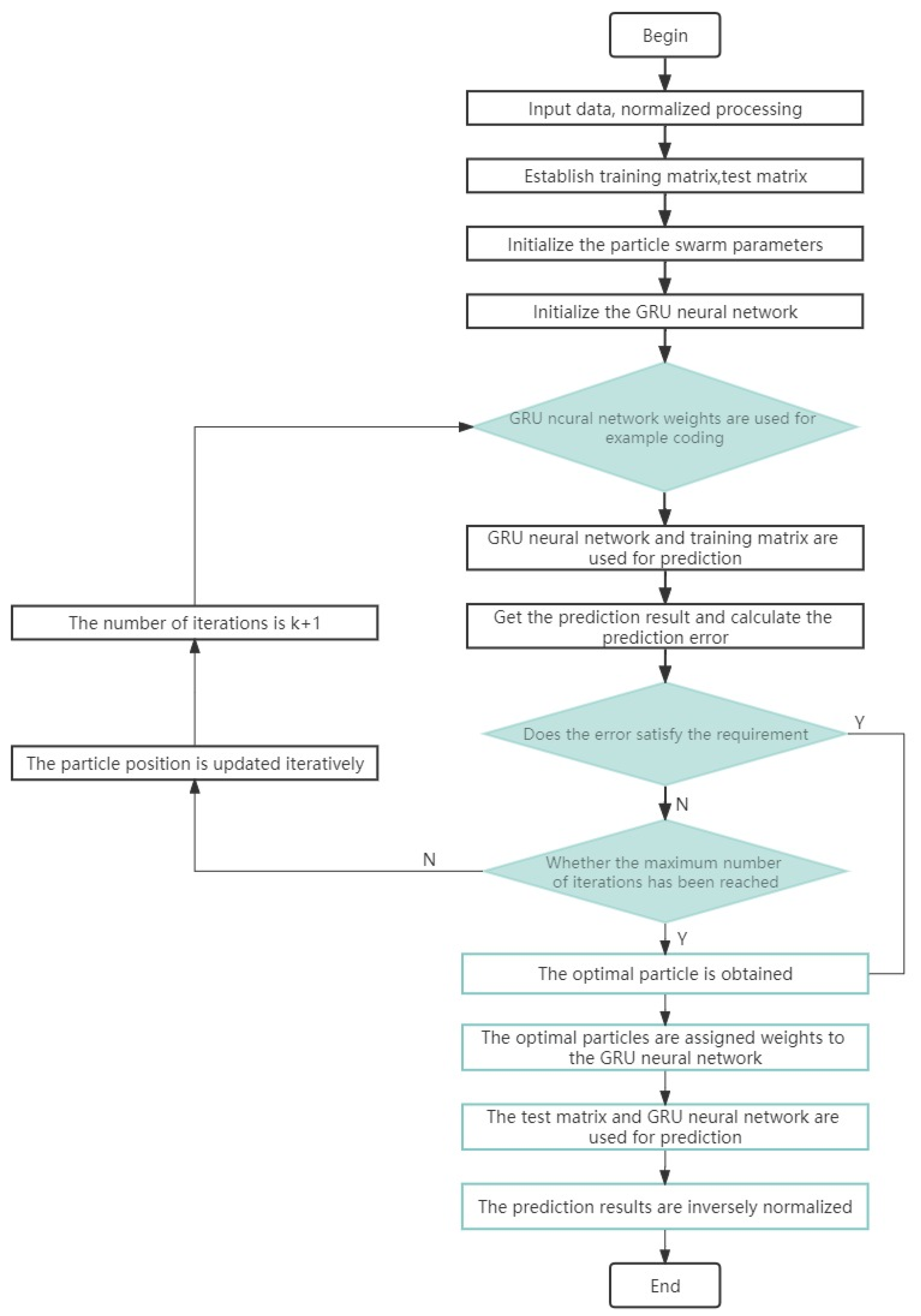
The prediction process of optimizing the GRU neural network based on particle swarm optimization (PSO) is as follows:

Step 1: perform abnormal value and normalization processing on input data and establish training matrix and test matrix.

Step 2: randomly generate the primary population and set the upper and lower limits of the parameters contained in each particle in the population.

Step 3: GRU network initialization, build GRU multi-load short-term forecasting model.

Step 4: particle code GRU network weights.

Step 5: use GRU neural network and training matrix to predict, calculate the error of output results, compare whether the error meets the requirements and whether the number of iterations reaches the maximum.

Step 6: repeat steps 4 and 5 to obtain the optimal particle.

Step 7: the optimized optimal particle is used for GRU network weight, the test matrix and GRU neural network are used for prediction and the prediction results are de-normalized.

For a more intuitive understanding of the calculation process, the algorithm process is shown in the following Figure 4.

3.3. Evaluation Indicators

For the evaluation of the effect of airport terminal load forecast value, an appropriate evaluation model is required. In this paper, four indicators are used to evaluate the forecast model: root mean square error (RMSE), mean square error (MSE), mean absolute error (MAE) and mean absolute percentage error (MAPE). All are used to evaluate the error between the measured value and the true value. The smaller the error is, the higher the accurate value is. The calculation formulas are as follows.

$$\mathrm{RMSE}=\sqrt{\frac{1}{\mathrm{n}}{\displaystyle \sum }_{\mathrm{i}=1}^{\mathrm{n}}({\mathrm{y}}_{\mathrm{i}}-{\hat{\mathrm{y}}}_{\mathrm{i}})2}=\sqrt{\frac{1}{\mathrm{n}}{\displaystyle \sum }_{\mathrm{i}=1}^{\mathrm{n}}{{\mathrm{e}}_{\mathrm{i}}}^2}\#$$

(9)

$$\mathrm{MSE}=\frac{1}{\mathrm{n}}{\displaystyle \sum }_{\mathrm{i}=1}^{\mathrm{n}}{({\mathrm{y}}_{\mathrm{i}}-{\hat{\mathrm{y}}}_{\mathrm{i}})}^2=\frac{1}{\mathrm{n}}{\displaystyle \sum }_{\mathrm{i}=1}^{\mathrm{n}}{\mathrm{e}}_{\mathrm{i}}{}^2\#$$

(10)

$$\mathrm{MAE}=\frac{1}{\mathrm{n}}{\displaystyle \sum }\left|{\mathrm{y}}_{\mathrm{i}}-{\hat{\mathrm{y}}}_{\mathrm{i}}\right|=\frac{1}{\mathrm{n}}{\displaystyle \sum }\left|{\mathrm{e}}_{\mathrm{i}}\right|\#$$

(11)

$$\mathrm{MAPE}=\frac{1}{\mathrm{n}}{\displaystyle \sum }_{\mathrm{i}=1}^{\mathrm{n}}\frac{\left|{\mathrm{y}}_{\mathrm{i}}-{\hat{\mathrm{y}}}_{\mathrm{i}}\right|}{{\mathrm{y}}_{\mathrm{i}}}\#$$

(12)

where n—verify the number of samples; i—i-th sample; ${\mathrm{y}}_{\mathrm{i}}$—predictive value; ${\hat{\mathrm{y}}}_{\mathrm{i}}$—actual value.

4. Results

4.1. Research Object

Taking the departure hall of the main building of an airport terminal in Shanghai as the research object, with a total area of 14,490 m², this study selects the time period from 6:00 a.m. to 22:00 p.m. from 1 July to 20 August as the research time. The research data are collected from the real data of the airport terminal (historical cooling load, indoor number of personnel), and the outdoor meteorological data (indoor temperature, solar radiation intensity, outdoor wind speed, relative humidity) are derived from the hourly data of China’s Meteorological websites. The training data are from 1 July to 15 August 2021, and the forecast data are from 16 August to 19 August.

4.2. Correlation Analysis

This paper used the spss26.0 platform to analyze the Pearson correlation coefficient, and selected input variables with strong correlation with the predicted cooling load. The number of cases is 785, and the correlation is Rxy and significance test values are shown in the

Table 3. Pearson correlation analysis between cooling load and input variable.

Cooling Load at Time T	Correlation Coefficient	Salience
The outdoor temperature at time T	0.281 *	0.046
Outdoor temperature at time T-1	0.257 *	0.069
Solar radiation intensity at time T	0.324 *	0.021
Solar radiation intensity at time T-1	0.332 *	0.017
Relative humidity at time T	−0.285 *	0.043
Outdoor wind speed at time T	0.025	0.844
Cooling load at time T-1	0.229 *	0.106
Cooling load at time T-2	0.06	0.673
Indoor temperature at time T	−0.085	0.553
Number of people in the room	1.00 **	0

Note: * at the 0.05 level, the correlation is significant; ** at the 0.01 level, the correlation is significant.

below:

When the correlation value is less than 0.2, but still significant, it indicates that the correlation is weak but still relevant. The point graph of cooling load correlation and significance at time t is as follows (Figure 5). The abscissa in the graph represents the input variable, and the ordinate represents the correlation value of the input variable and cooling load at time t.

According to the above chart, it can be clearly found that the correlation of outdoor wind speed at time t is 0.025. In summer, the unorganized infiltration caused by wind pressure has little impact on indoor temperature and has very little impact on indoor cooling load prediction. Therefore, the correlation is poor. The correlation of cooling load at time T-2 is 0.06, and the correlation is very weak, mainly because the historical cooling load in the previous two hours had a low cooling effect with the flow of people, compared with other inputs. The influence of cooling load at time T-2 is very small. The indoor temperature of the airport terminal at time t is negatively correlated, with a correlation value of 0.085. The correlation is very weak. The results show that the relationship between cooling load prediction and indoor temperature change is weak. To sum up, this paper discards the input variables with very weak correlation, and selects the input variables “the outdoor temperature at time t, outdoor temperature at time t-1, solar radiation intensity at time t, solar radiation intensity at time t-1, relative humidity at time t, cooling load at time t-1, number of people in the room at time T”. Among them, the correlation coefficient between the number of people in the room and the cooling load at time T is 1, which shows that the passenger flow in the terminal has a great impact on the indoor cooling load.

4.3. Discussion

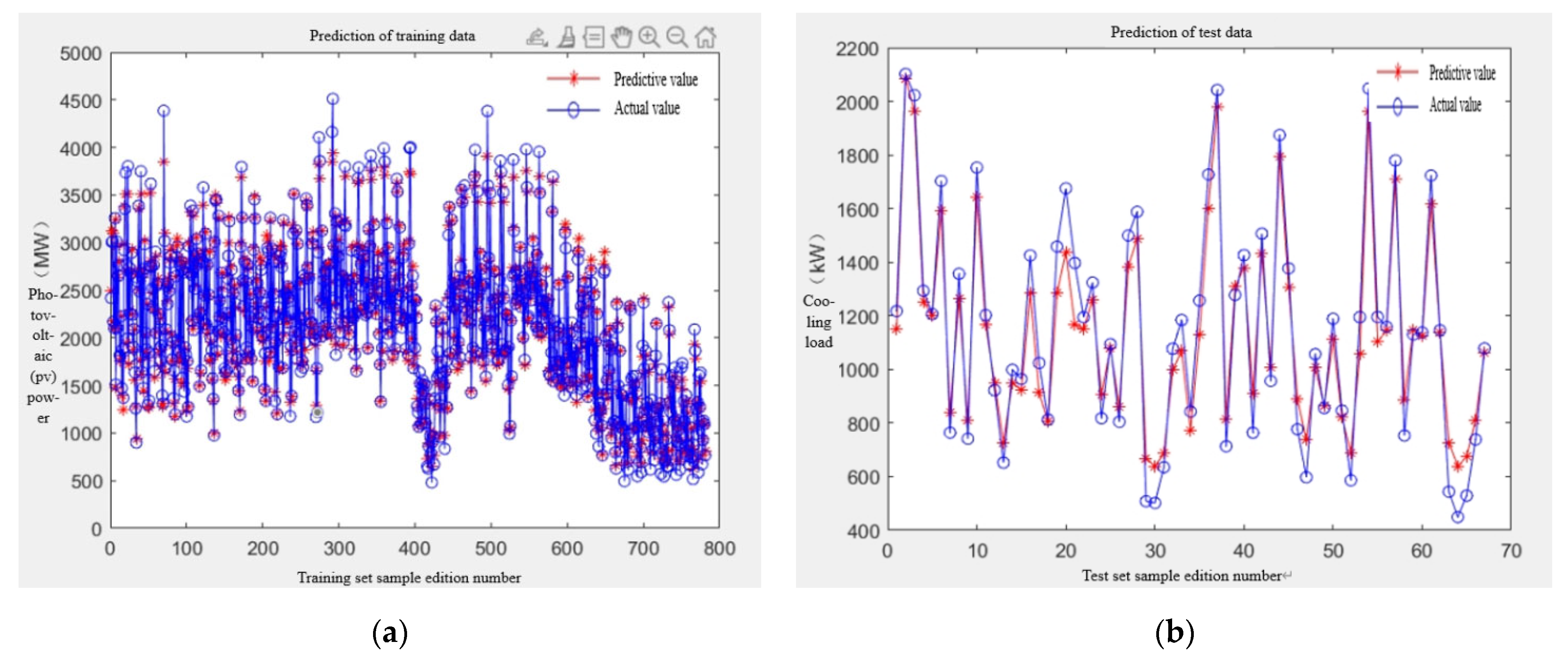
On the basis of Pearson correlation analysis, this paper uses MATLAB software programming and the PSO-GRU model for prediction. In order to verify the accuracy of the model, LSTM, PSO-LSTM, CNN-LSTM, PSO-CNN-LSTM and GRU prediction models are used for comparison. The convolutional neural network (CNN) and LSTM network can complement each other’s characteristics. CNN is used to extract the potential relationship between continuous and discontinuous data in the input historical data, and the LSTM network model is used for short-term prediction. The accuracy of power load prediction is higher than that of a single LSTM network [18]. The maximum number of iterations of neural network is 500, and the learning rate is 0.005.The hourly training data and test data of the LSTM model, GRU model and CNN-LSTM model during the research period can be seen in the Figure 6, Figure 7 and Figure 8.

By comparing the training data and test data prediction charts of the three models, it can be found that the fitting degree of the LSTM and GRU models is high, and the fitting degree of the CNN-LSTM model is the worst. For the cooling load of the airport terminal, CNN extracts the local characteristic parameters of historical load with half the accuracy. Among them, compared with other models, the GRU model is obviously more accurate in details, especially at sampling point 30, and the fitting of the GRU model is significantly higher than that of the LSTM model. In general, for the prediction of airport terminal cooling load, the GRU model has higher prediction accuracy, and as Ma [27] and others put forward, the GRU network has simpler structure, fewer parameters, easier convergence and faster training speed, and its training time is less than the LSTM model, which is feasible, but there are fluctuations in details, which can be optimized.

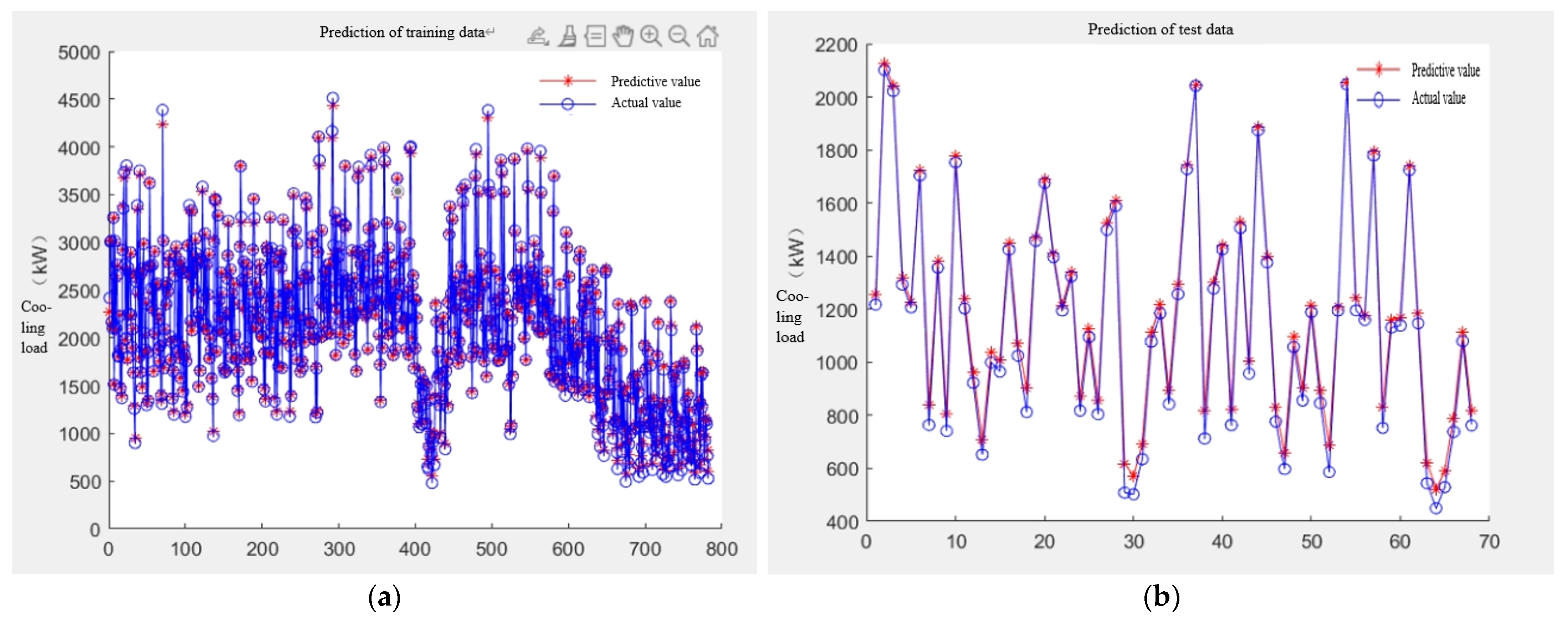
In this paper, the particle swarm optimization algorithm was selected to optimize the number of neurons m and time step t in the GRU network model. The number of neurons and time steps are taken as the characteristics of particle optimization, and the optimal solution is calculated by the PSO algorithm. In this paper, RMSE, MSE, Mae and MAPE are selected as the reference for error analysis. In the experiment, the PSO algorithm c1 = 1.5, c2 = 1.5, the population size is 10, the maximum number of iterations is 500, Vmax is 1 and the inertia weight w = 0.2. The model prediction diagram optimized by PSO is shown in the following Figure 9, Figure 10 and Figure 11.

As shown in the figure above, the PSO-optimized model has less fluctuation than a single model. Comparing the three prediction models of PSO-CNN-LSTM, PSO-LSTM and PSO-GRU, the latter two’s actual and predicted values fit better, especially at the sampling point 30, the PSO-CNN-LSTM fluctuates significantly and the PSO-LSTM and PSO-GRU models have high prediction accuracy, but, in the details, the PSO-GRU model fluctuates very little, which is more accurate than the other two models. One point can be intuitively reflected by the error evaluation index. The error comparison of different models is shown in the following

Table 4. Error comparison of different prediction models.

Predictive Model	RMSE	MSE	MAE	MAPE
LSTM	40.1703	1613.6566	34.7746	0.038122
PSO-LSTM	17.8768	319.5788	12.843	0.012873
CNN-LSTM	99.1324	9827.2383	83.3895	0.0830
PSO-CNN-LSTM	63.2905	4005.6861	48.1674	0.051107
GRU	12.227	149.4997	9.8208	0.011321
PSO-GRU	11.1881	125.1739	7.7116	0.0079067

.

It can be seen from the above table that the error of the model optimized by the PSO algorithm is significantly smaller than that of the model not optimized. Taking the average absolute percentage error (MAPE) as an example, the absolute error of GRU not optimized by PSO is 1.1%, which is 0.1% lower than that of the LSTM model optimized by PSO, while the error of the CNN-LSTM model is the largest, which is 8%; even after optimization, the error is 2% higher than that of the LSTM model. The prediction effect of the PSO-GRU model is the best, and the error is only 0.7%. At the same time, as Yang [28] and others said, compared with the GRU model, the PSO-GRU model has faster convergence speed, better calculation efficiency and accuracy and is feasible. It can be seen that the GRU neural network model based on the PSO algorithm is selected for airport terminal cooling load forecasting, which has the best effect and the highest prediction accuracy.

5. Conclusions

This paper presents a GRU neural network prediction model based on the particle swarm optimization algorithm for airport terminal cooling load, analyzes the correlation of influencing factors through the Pearson correlation analysis method, compares the prediction effects of different neural network models, uses the particle swarm optimization algorithm to optimize the neural network super parameters and structure, and finds the optimal model.

The results show that: (1) Outdoor temperature, relative humidity, solar radiation intensity, cooling load at historical time and the number of indoor personnel have a greater correlation with the cooling load of the terminal; (2) Comparing LSTM, GRU and CNN-LSTM, the three neural network models, the average absolute percentage error of the GRU neural network prediction is only 1.1%, and the accuracy is the highest; (3) The accuracy of the neural network model optimized by the particle swarm algorithm (PSO) has been improved, compared with the optimized PSO-LSTM, PSO-CNN-LSTM and PSO-GRU prediction models, the average absolute percentage error of the PSO-GRU model is only 0.7%, the prediction accuracy is high, the effect is optimal, and the cooling demand is accurately controlled.

In this paper, the passenger flow is considered as the number of people at the current time, but passenger flow and flight delay have a great relationship. On this basis, it is necessary to integrate the predicted passenger flow to further improve the large space load forecasting model and improve the prediction accuracy.

References

- Khudhair, A.M.; Farid, M. A review on energy conservation in building applications with thermal storage by latent heat using phase change materials. Therm. Energy Storage Phase Chang. Mater. 2021, 45, 162–175. [Google Scholar] [CrossRef]
- Wei, W.; Wei, Q.; Zhang, H.; Lu, D.; Liang, M. Research and application of operation control strategy of airport terminal cold source system based on load forecasting. Build. Energy Effic. (Chin. Engl.) 2022, 50, 50–56. [Google Scholar]
- Tang, Z. Research and Implementation of Short-Term Load Forecasting for Local Power Grid. Master’s Thesis, Guangxi University, Nanning, China, 2008. [Google Scholar]
- Zhao, S. Research on Short-Term Power Load Forecasting Method Based on Incremental Association Rule Algorithm. Master’s Thesis, Nanjing University of Posts and Telecommunications, Nanjing, China, 2018. [Google Scholar]
- Li, C.; Zhang, B.; Chen, Y.; Lv, B.; Yang, Y.; Wang, H. Application of convolution enhanced recurrent neural network in text classification. J. Xianyang Norm. Univ. 2021, 36, 24–29. [Google Scholar]
- Ren, P. Prediction of Short-Term Check-In Passenger Flow of Airport Based on Time Series. Master’s Thesis, Civil Aviation University of China, Tianjin, China, 2019. [Google Scholar]
- Zheng, R.; Zhang, S.; Xiao, X.; Wang, Y. Short term load forecasting based on multi-layer long short memory neural network considering temperature fuzziness. Power Autom. Equip. 2020, 40, 181–186. [Google Scholar]
- Xie, Y. Research on Load Forecasting and Multi Heat Source Optimal Scheduling of Heating System in an Airport Terminal. Master’s Thesis, Xi’an University of Architecture and Technology, Xi’an, China, 2021. [Google Scholar]
- Gong, T. Research on Short-Term Load Forecasting Based on MDS and PSO-GRU Neural Network. Master’s Thesis, Hubei University of Technology, Wuhan, China, 2021. [Google Scholar]
- Tang, X.; Dai, Y.; Wang, T.; Chen, Y. Short-term power load forecasting based on multi-layer bidirectional recurrent neural network. IET Generation. Transm. Distrib. 2019, 13, 3847–3854. [Google Scholar] [CrossRef]
- Zhao, B.; Wang, Z.; Ji, W.; Gao, X.; Li, X. CNN-GRU short-term power load forecasting method based on attention mechanism. J. Med. Syst. 2019, 12, 4370–4376. [Google Scholar]
- Lin, L.; Liu, X.; Zhang, T.; Liu, X.; Rong, X. Cooling load characteristic and uncertainty analysis of a hub airport terminal. Energy Build. 2021, 231, 110619. [Google Scholar] [CrossRef]
- Wang, X.; Feng, W.; Cai, W.; Ren, H.; Ding, C.; Zhou, N. Do residential building energy efficiency standards reduce energy consumption in China?—A data-driven method to validate the actual performance of building energy efficiency standards. Energy Policy 2019, 131, 82–98. [Google Scholar] [CrossRef]
- Liu, X.; Lin, L.; Liu, X.; Zhang, T.; Rong, X.; Yang, L.; Xiong, D. Evaluation of air infiltration in a hub airport terminal: On-site measurement and numerical simulation. Build. Environ. 2018, 143, 163–177. [Google Scholar] [CrossRef]
- Liu, X.; Li, L.; Liu, X.; Zhang, T. Analysis of passenger flow and its influences on HVAC systems: An agent T based simulation in a Chinese hub airport terminal. Build. Environ. 2019, 154, 55–67. [Google Scholar] [CrossRef]
- Eshtaiwi, M.; Badi, I.; Abdulshahed, A.; Erkan, T.E. Determination of key performance indicators for measuring airport success: A case study in Libya. J. Air Transp. Manag. 2018, 68, 28–34. [Google Scholar] [CrossRef]
- Kotopouleas, A.; Nikolopoulou, M. Evaluation of comfort conditions in airport terminal buildings. Build. Environ. 2018, 130, 162–178. [Google Scholar] [CrossRef]
- Li, J.; Xu, W.; Zhang, X.; Feng, X.; Chen, Z.; Qiao, B.; Xue, H. Control method of multi-energy system based on layered control architecture. Energy Build. 2022, 261, 111963. [Google Scholar] [CrossRef]
- Wang, R.; Li, Z.; Cao, J.; Chen, T.; Wang, L. Convolutional recurrent neural networks for text classification. In Proceedings of the 2019 International Joint Conference on Neural Networks (IJCNN), Budapest, Hungary, 14–19 July 2019; pp. 1–6. [Google Scholar]
- Zhu, S.; Zhao, Y.; Zhang, Y.; Li, Q.; Wang, W.; Yang, S. Short-term traffic flow prediction with wavelet and multi-dimensional taylor network model. IEEE Trans. Intell. Transp. Syst. 2020, 22, 3203–3208. [Google Scholar] [CrossRef]
- Shang, C.; Gao, J.; Liu, H.; Liu, F. Short-term load forecasting based on PSO-KFCM daily load curve clustering and CNN-LSTM model. IEEE Access 2021, 9, 50344–50357. [Google Scholar] [CrossRef]
- Yuan, X.; Chen, C.; Jiang, M.; Yuan, Y. Prediction interval of wind power using parameter optimized beta distribution based LSTM model. Appl. Soft Comput. 2019, 82, 105550. [Google Scholar] [CrossRef]
- Ahn, Y.; Kim, B.S. Prediction of building power consumption using transfer learning-based reference building and simulation dataset. Energy Build. 2022, 258, 111717. [Google Scholar] [CrossRef]
- Phyo, P.P.; Jeenanunta, C. Advanced ML-Based Ensemble and Deep Learning Models for Short-Term Load Forecasting: Comparative Analysis Using Feature Engineering. Appl. Sci. 2022, 12, 4882. [Google Scholar] [CrossRef]
- Liu, X.; Li, L.; Liu, X.; Zhang, T.; Rong, X.; Yang, L.; Xiong, D. Field investigation on characteristics of passenger flow in a Chinese hub airport terminal. Build. Environ. 2018, 133, 51–61. [Google Scholar] [CrossRef]
- Li, D.; Sun, G.; Miao, S.; Gu, Y.; Zhang, Y.; He, S. A short-term electric load forecast method based on improved sequence-to-sequence GRU with adaptive temporal dependence. Int. J. Electr. Power Energy Syst. 2022, 137, 107627. [Google Scholar] [CrossRef]
- Ma, Y.; Xiao, J.; Shao, L.; Ma, Y.; Zuo, X.; Zhang, H. Research on Temperature and Humidity Prediction Model of Printing Workshop Based on LSTM and GRU Network Integration. Digital Print. 2022, 3, 34–41. [Google Scholar] [CrossRef]
- Yang, Y.; Du, J.; Wu, Y. Temperature prediction based on PCA and improved PSO-GRU neural network. Mod. Electron. Technol. 2022, 45, 89–94. [Google Scholar] [CrossRef]