Article

Research on the Factors of Pedestrian Volume in Different Functional Areas of Kumamoto City

1
Graduate School of Science and Technology, Kumamoto University, 2-39-1 Kurokami, Chuo-ku, Kumamoto 860-8555, Japan
2
Faculty of Advanced Science and Technology, Kumamoto University, 2-39-1 Kurokami, Chuo-ku, Kumamoto 860-8555, Japan
3
Institute of Policy Research, 9-24 Hanabata Chuo-ku, Kumamoto 860-8555, Japan
4
School of Tourism and Urban-Rural Planning, Zhejiang Gongshang University, Hangzhou 310018, China
*
Author to whom correspondence should be addressed.
Sustainability 2022, 14(18), 11636; https://doi.org/10.3390/su141811636
Submission received: 25 July 2022 / Revised: 3 September 2022 / Accepted: 15 September 2022 / Published: 16 September 2022

Abstract

:
Improving urban walkability is critical to the long-term development of cities. Although previous studies have demonstrated a relationship between the built environment and walking, an approach that can control the exploration of different functional areas has not yet been discussed. In this study, built environment features include density, design, diversity, destination accessibility, and distance to transit. Geodetector and regression methods were used to investigate the impact of the built environmental features on pedestrian volume in different functional areas of Kumamoto City. It was found there were various dominant features for the different functional areas in the city, including the city center (diversity, design, and density), local hubs (destination accessibility, density, and distance to transit), living hubs (density, design, and distance to transit), UPA (diversity, design, and distance to transit), UCA (density, density, and design), and NPA (density). Additionally, population density and land use diversity in the overly dense population area were negatively related to pedestrian volume. This study complements research on pedestrians and the built environment in different functional areas, and provides advice for the urban planners and government of Kumamoto City.

1. Introduction

Japan differs significantly from Europe and the United States; Japan has densely developed cities with a high-density urban road network. With the decline in population, low birth rate, and an aging society, there are concerns that Japanese urban vitality will decline in regional vitality due to shuttered shopping streets. The city infrastructure is no longer adequate for pedestrian demand. Owing to COVID-19, the emergency declaration further reduced the number of pedestrians in the city. In 2020, the Japanese government proposed a walkability promotion program for city center renovations [1]. This program includes using redistributed road space, scenery, greenery, and the overall environment. Understanding how built environmental factors influence walking behavior can help governments and urban planners to make good decisions to improve the vitality of cities.
Kumamoto City is one of the cities being put forward for the walkability promotion program. According to a survey on the Kumamoto Metropolitan Area’s urban transportation master plan, 75% of the elderly are dissatisfied with the built environment for walking [2]. Improving the built environments of Kumamoto City is necessary. One criterion to evaluate the walkability of the streets involves determining the number of pedestrians [3]. Assessing population-level walking behavior allows interventions to be developed in urban planning to promote physical activities [4]. Pedestrian volume is a population-level walking behavior [4]. Understanding the influencing factors from the built environment on pedestrian volume can help develop a better walkable environment.
Walking has benefits for both health and creating fewer carbon emissions. According to previous research, decreased walking activity due to factors in the built environment adversely impacts people’s health [5,6]. The lack of walking is a risk factor for several cardiovascular diseases [7]. Interrupting sitting time with short and frequent light-intensity walking improves cardiometabolic health [8]. The daily addition of 1000 extra steps from walking can help reduce all-cause mortality, cardiovascular disease morbidity, and mortality in adults [9]. Besides being beneficial to health, walking helps reduce carbon emissions [10]. Walking or cycling can replace 41% of short-distance car trips, reducing carbon emissions from car trips by nearly 5% [11]. It also moderately reduces air pollution [12]. Therefore, promoting the development of walkable cities is essential for sustainable development.
Although numerous studies have observed the relationship between walking and the built environment, some gaps, which deserve research attention, remain. Previous studies have demonstrated the relationship between the built environment and walking, but an approach that can control the exploring of different functional areas has not been discussed. The independent variables are the built environment features, and the independent variable is pedestrian volume. This study uses regression models and Geodetector [13] to investigate the built environment’s impact on population-level walkability.
Compared with previous studies, this study has the following innovations: (1) exploring the impact of the built environment on pedestrian volume from various functional areas of the city and (2) discussing the interaction of different built environment features on pedestrian volume. Research contributions include the following. Firstly, this work contributes to the built environment and pedestrian volume studies by focusing on the built environment features of different functional areas at the urban scale. Secondly, this study complements the interaction of built environment features within the study of built environments. Our findings on spatial differences during the impact of built environment features on pedestrian volume (in different functional areas) will help urban planners and governments to improve the planning and management of the built environment.

2. Literature Review

2.1. Built Environment and Walking

The built environment features include density, diversity, design, destination accessibility, and distance to transit, which can be referred to as the five “D” (5D) features [4,14,15,16]. The land use mixture or the mixed entropy of land use belongs to diversity [14,15]. Design covers street network characteristics and the streetscape within an area [14,15,17]. In the 1960s, Jacobs criticized urban planning and proposed the impact of primary mixed uses (diversity), small blocks, and aged buildings (design) on pedestrians [18]. Then, density was presented, which meant the variable of interest per unit of area, such as population, residential units, and employment [14]. In the 1990s, Cervero and Kockelman [15] proposed that travel demand was affected by three variables of the built environment: density, diversity, and design (3Ds).
Furthermore, Lee and Moudon considered the route based on the 3D variables [16]. Ewing and Cervero added distance to transit and destination accessibility to the three variables and proposed a 5D framework [14]. In addition, Saelens et al. [19] proposed the concept of walkability and found environmental factors, such as population density, road connectivity, and land use mixture. Southworth [17] presented six walkable city attributes: road connectivity, fine-grained land use patterns, linkage with other modes, safety, path quality, and path context.
Some scholars have discussed how to use the built environment to measure walkability. Frank [20,21] created the walkability index using residential density, land use diversity, and intersection density. Carr et al. [22] proposed the walk score [23], using destination accessibility, intersection density, and block length. However, these two indicators were developed in the United States and may not be suitable in Asian countries, such as Japan. Therefore, Hino et al. [24] proposed the Japanese walkability index based on destination accessibility and compared it with Frank’s walkability index. Koohsari et al. [25] verified the walk score in Japan by using housing density, number of local destinations, intersections, access to public transportation, and pedestrian availability. Kato and Kanki [26] developed a walkability indicator for predicting the future population, composed of housing density, amenity accessibility, road connectivity, and safety for shrinking cities in Japan.
In addition, scholars have focused on the impact of the streetscape on walking. Kim et al. [27] investigated the effects of built environment variables on pedestrian satisfaction using questionnaires, such as sidewalk width, the presence of bus lanes, lights, and greeneries. Due to the development of computer vision and the usage of street view images, some research has shifted from self-reported studies to the quantitative measurement of the built environment. According to evidence from Hong Kong, the number of parks and eye-level street greenery, calculated by streetscape analysis, were related to higher odds of walking, and eye-level street greenery was related to total walking time [28]. In a study on leisure walking, Nagata et al. [29] discovered that active elderly female walkers were associated with streetscape walkability, as predicted by the street elements. Additionally, Zhou et al. [30] analyze social inequality to facilitate healthy city planning by calculating neighborhood visual walkability, including greenery, visual crowding, enclosure, and visual pavement.

2.2. Pedestrian Volume

There was a correlation between pedestrian volume and the built environment [4,31]. Pedestrian volume can assess walkability and pedestrian activity based on the pedestrian count [32,33]. Some researchers have attempted to reduce the time and money consumed by pedestrian volume counting methods, such as using street view data for pedestrian volume measuring methods. Yin et al. [34] counted pedestrians using Google Street View images and used manual counting to adjust the pedestrian volume with reasonable accuracy. Furthermore, video counting has confirmed the effectiveness of pedestrian volume from street-view data counting [35]. Through the pedestrian volume counting of Shanghai Street View images, Chen et al. [4] discovered that the micro- and macro-scale built environments affected pedestrian volume. Furthermore, the method of collecting pedestrian data via Street View images was applied to study the collective walking behavior and built environment features [36].

3. Research Area and Data

3.1. Research Area

Kumamoto City is one of Japan’s “compact cities”, with high-density development, having an area of 390 km2 and a population of 737,219 as of May 2022. In 2020, the Ministry of Land, Infrastructure, Transport and Tourism of Japan established a walkable city to promote regional vitality. Kumamoto City is one of 53 cities that have been set up as a walkable area.
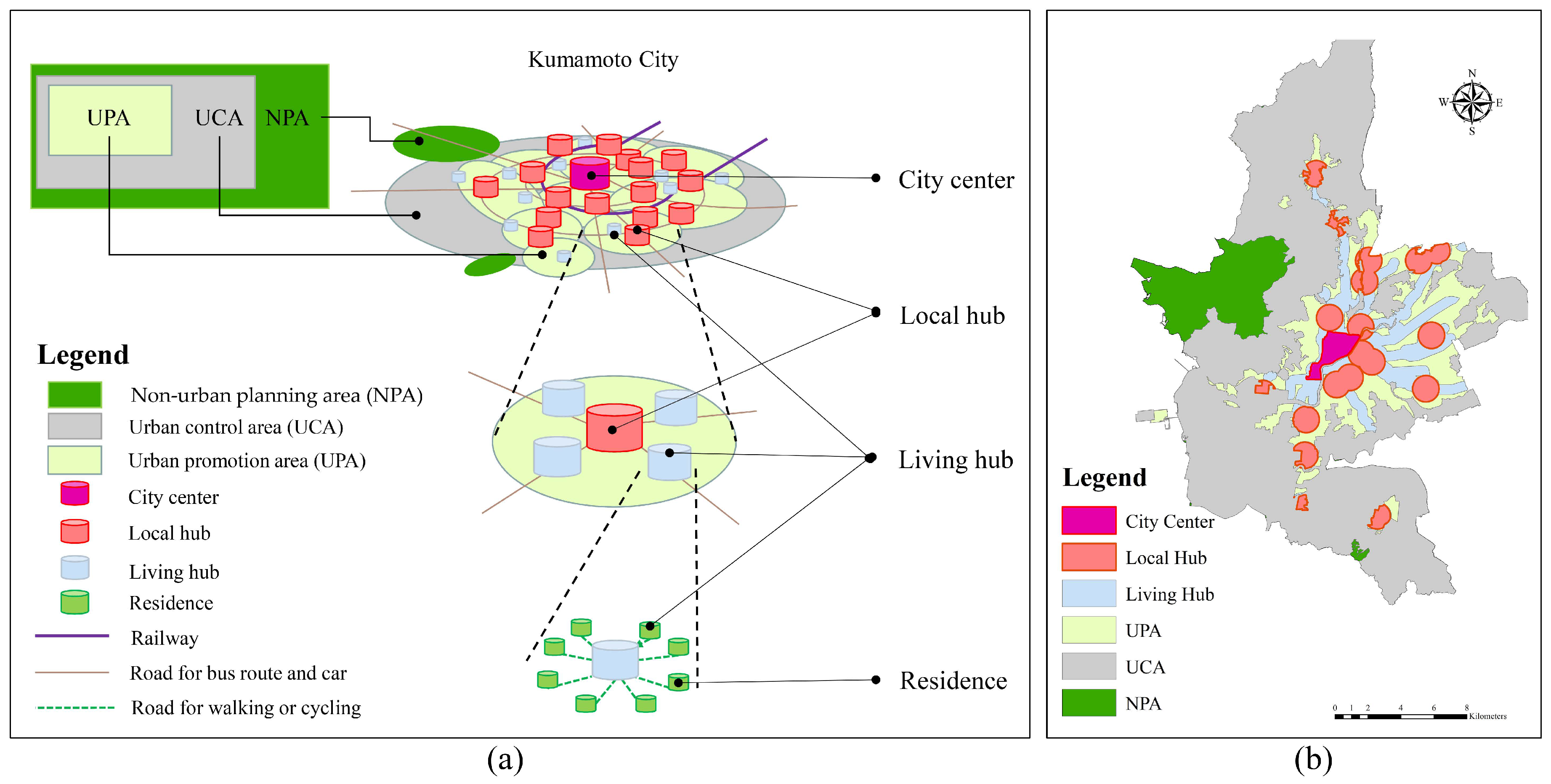
According to the compact city planning of Kumamoto City [37], the functional areas include urban function promotion areas (city center), urban function promotion areas (local hub), residential promotion areas (living hub), urban promotion areas (UPA), urban control areas (UCA), and non-urban planning areas (NPA) [38]. Figure 1 shows the research area.
The city center begins from Kumamoto Castle and the area around the city hall to the Kumamoto Station, which measures approximately 415 ha. The city center has concentrated urban functions that promote the development of social and economic activities, such as business, commerce, arts and culture, and exchanges. The local hub is within the 15 core districts in Kumamoto City, within an 800 m radius. The local hub is where essential urban functions, such as commercial, administrative services, medical care, welfare, and education, are concentrated. The living hub is where citizens independently conduct community activities. Finally, the living hub has private shops, public halls, and elementary and junior high schools.
The UPA is a lively urbanized area with many houses and shops. The UCA is an urban planning area that needs to be developed or preserved to form a cohesive city that is centered on an urban area. The NPA is not within the urban planning area. The research area uses a 250 m fishing net for the minimum population statistical scale as the research unit, obtained from the portal of official statistics in Japan, e-stat (www.e-stat.go.jp, accessed on 24 July 2022).

3.2. Research Data

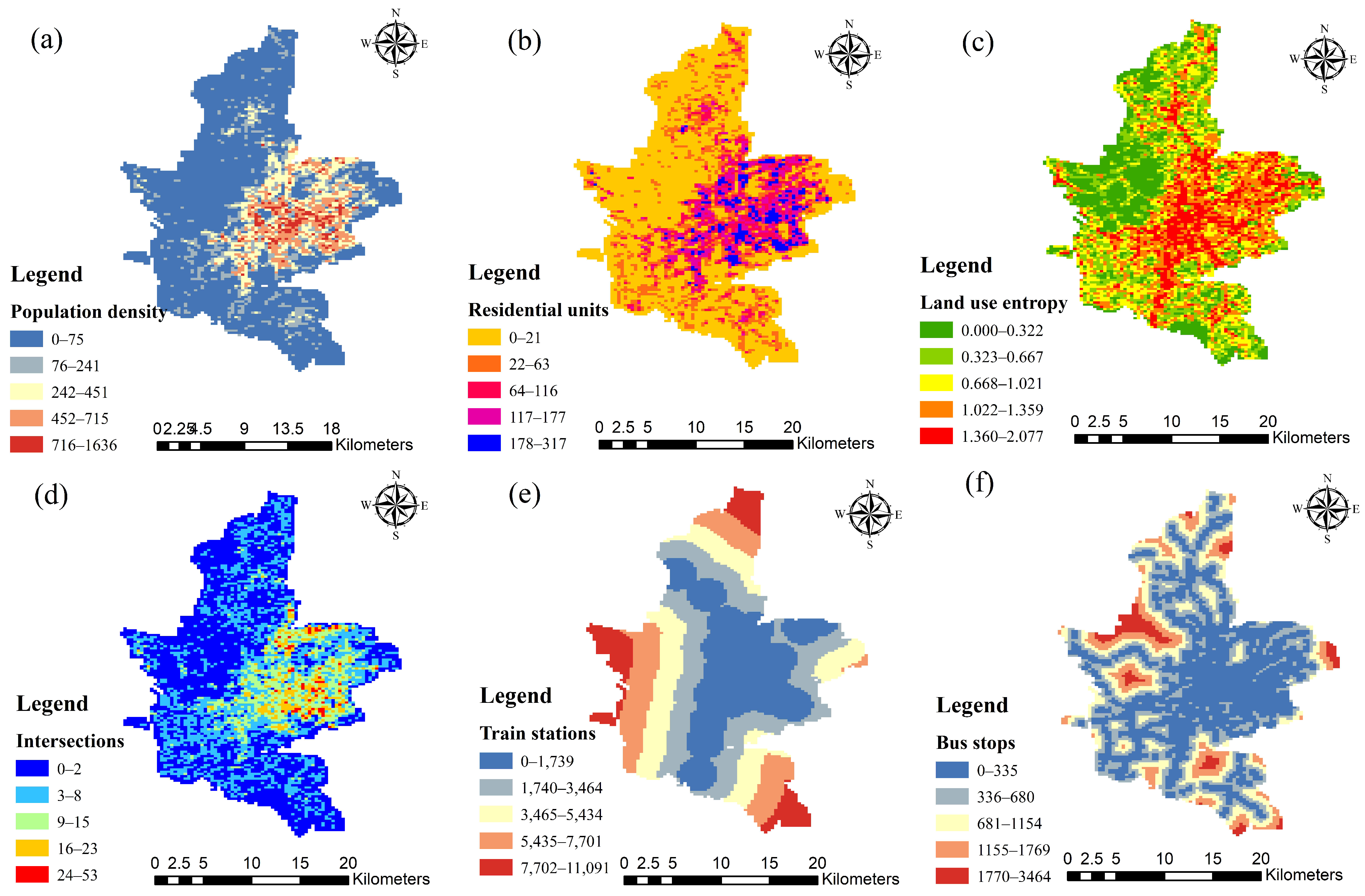
The independent variables (the built environment) include density, diversity, design, destination accessibility, and distance to transit. The dependent variable was the pedestrian volume. The research data and sources are categorized as shown in Table 1. Figure 2 shows some of the data.
Diversity includes land use entropy and the ratio of working and living population. The land use types include agricultural and natural land, water bodies, residential land, commercial land, industrial land, land of public facilities, roads, land of transportation facilities, public open space, and public facilities land. The land use entropy was calculated using Equation (1).
Land   use   entropy = i = 1 n p i × ln p i
where p i is the i th land area’s ratio to the area of the chunk, and n is the total land use type in the chunk.
Residential units are the number of residential buildings per unit area. Population density is the number of populations per unit area. Street View data were collected using a road network every 50 m along all streets in the research area, including the starting and ending points. The images were collected from 74,535 locations using different angles: 0, 90, 180, and 270°. We gathered 298,140 Street View images, which were 800 × 800 pixels. Destination accessibility includes groceries (369), restaurants (2739), shopping (1410), entertainment facilities (90), libraries (35), fitness facilities (87), banks (471), hospitals (1142), parks (881), and schools (193). Distance to transit includes bus stops (1050) and train stations (62).

4. Methods

4.1. Destination Accessibility

Destination accessibility contains regional accessibility and local accessibility [14]. Local accessibility is obtained by calculating the accessibility to amenities within a given travel time. According to the walk score methodology and Japanese research [22,23,24,25,26], the following amenities are selected as local accessibility destinations, as shown in Table 2.
The scores for restaurants and shopping are combined with the weighting of calculating the scores using multiple facilities, which is influenced by the choices and types [23]. The closer the distance, the greater weighting. The weight values for restaurants and shopping facilities are obtained by scaling the weights for different restaurants and shopping in the walk score methodology. The amenity weights of shopping were 0.25, 0.225, 0.2, 0.175, and 0.15. The amenity weights for restaurants were 0.25, 0.15, 0.1, 0.1, 0.075, 0.075, 0.075, 0.075, 0.05, and 0.05. Other amenities use the nearest facility to calculate their accessibility score.
The amenity accessibility score decreased with the walking distance, remaining within 5 min, rapidly reducing from 5 to 20 min and became 0 when it exceeded 30 min [22,23]. According to Kumamoto City’s compact city planning, the 800 m circle for the local hub requires 10 min of walking time, which translates to a walking speed of 80 m per minute. Therefore, the walking distances in the three phases are 400, 1600, and 2400 m. Equation (2) shows the delay function as fit by the Gaussian function.
We calculated the actual walking distance using the OD cost matrix of network analysis based on the road network and amenities of the destination. The amenity accessibility score decreases from short to long distances.
AS = { 100 ,                                         distance < 400   m 100 × e ( x 0.4 ) 2 2 × 0.65 2 ,                 400   m distance 2400   m 0 ,                                         distance > 2400   m    
Here, AS represents the score of amenity accessibility and x represents the walking distance of amenity.

4.2. Landscape Detection

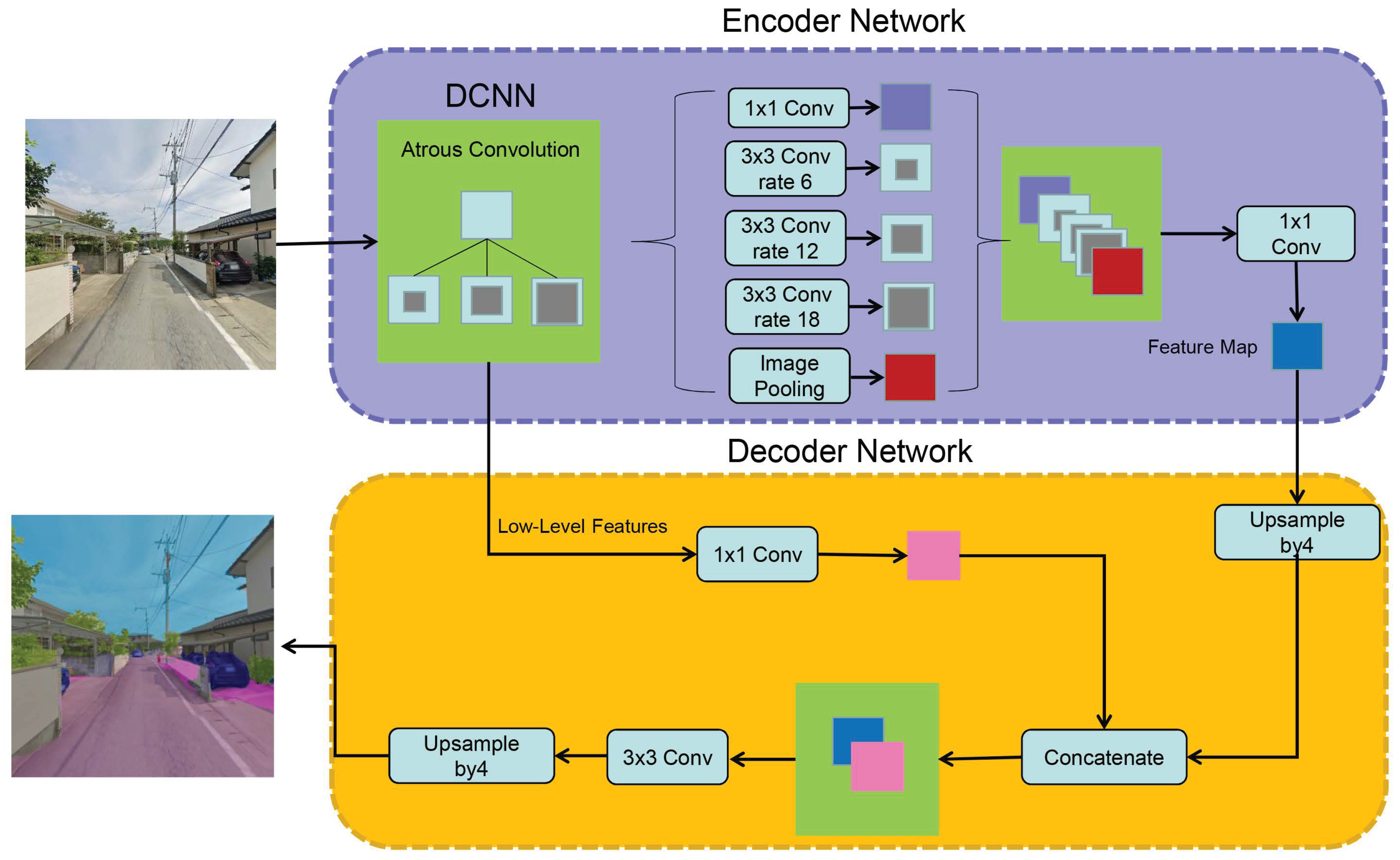
The Deeplab V3+ neural network [39] was developed using python 3.6, as shown in Figure 3. The backbone network was ResNet-101. A pre-trained model was obtained by training using the Cityscapes Dataset (www.cityscapes-dataset.com, accessed on 24 July 2022). However, in this study, the vegetation ratio was used as greenery, sky ratio was used as open sky, building ratio was used as eye-level building, and road ratio was used as eye-level road. The ratio of point location was calculated using four angled images.

4.3. Target Detection

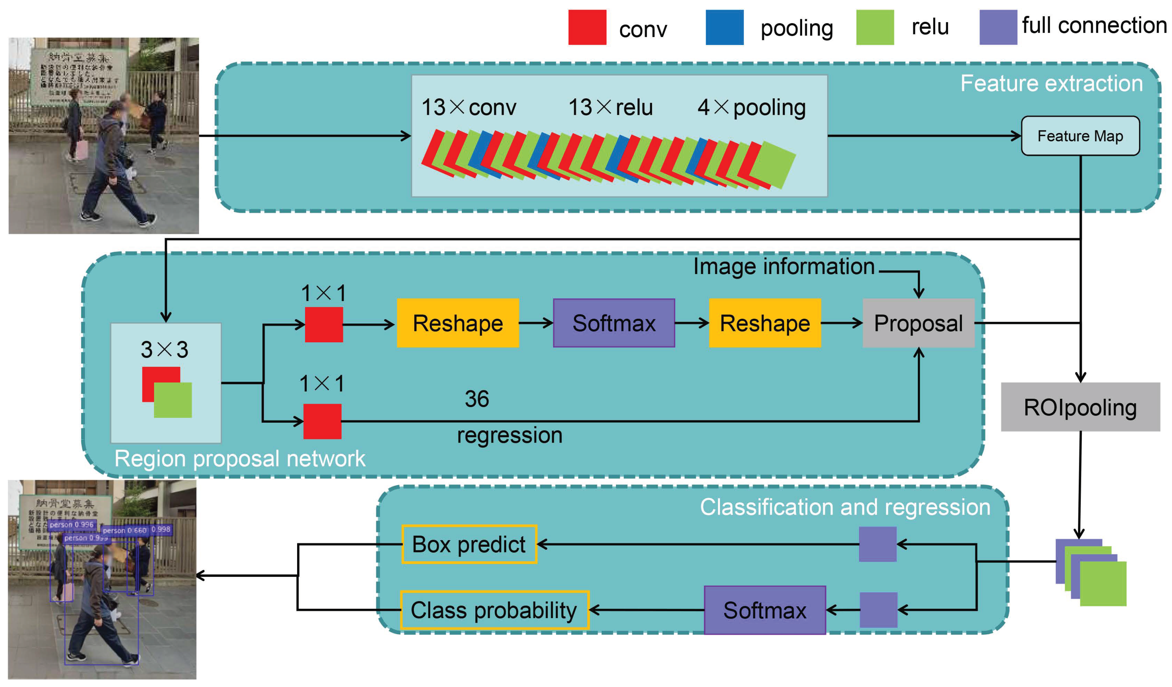
The pre-trained model for the Faster-RCNN neural network [40] was developed in python 3.6 and trained using the Pascal VOC Dataset (host.robots.ox.ac.uk/pascal/VOC, accessed on 24 July 2022), as shown in Figure 4. The pedestrian volume was calculated by counting the number of pedestrians at each point within a 250 m chunk.

4.4. Regression Models

4.4.1. Ordinary Least Squares Regression

According to the various functional areas, we create seven datasets: city, local hub (LOH), living hub (LOH), UPA, UCA, and NPA. The normalization and ordinary least squares (OLS) regression are performed to analyze the relationship between the built environment features and pedestrian volume, as shown in Equations (3) and (4).
X * = X X m i n X m a x X m i n ,   Y * = Y Y m i n Y m a x X m i n
Y = a 1 X 1 * + a 2 X 2 * + + a 20 X 20 * + a 21 X 21 * + b
where X represents the 21 categories of independent variables, Y is the dependent variable, X * and Y * mean the normalization of X and Y , a is the regression coefficient, and b is a constant.

4.4.2. Spatial Lag Model

Spatial data are spatially dependent, meaning that the number of pedestrians observed at one location depends on the number of pedestrians observed at neighboring sites. Considering that the spatial distribution of the pedestrians has an autocorrelation, the spatial lag model (SLM) was selected, as shown in Equation (5).
y i = β x i + ρ w y i + μ i
where x i is the independent variable at model i , y i represents the value of the dependent variable at model i, β is the intercept, ρ is the spatial autocorrelation parameter, w y i is a spatial weight matrix of the dependent variable at model i. μ i is random error terms.

4.5. Geodetector

Geodetector [13] is an essential tool for studying the spatial differentiation of natural and socioeconomic processes. It can analyze the interactions between variables and investigate spatial differentiation. Geodetector contains factor detector, risk detector, ecological detector, and interaction detector. It can detect the interaction of two factors on the dependent variable and can confirm whether an interaction is between the two factors.

4.5.1. Jenk’s Breaks Classification

Using Jenk’s breaks classification, the differences between the groups are apparent. Even the disagreements within the data are minor, and each group has a clear break. Jenk’s Breaks classification uses a traversal method to calculate data one by one until reaching the minimum cluster distance, as shown in Equations (6) and (7).
E = i = 1 k x C i x μ i 2
μ i = 1 | C i | x C i x
where x represents the input variable, k represents the number of clusters the samples will be divided into, such as C 1 ,..., C k . E is the objective function of the classification method, which needs to be minimized. μ i is the mean vector of the cluster C i .
All independent variable data were divided into five subareas by Jenk’s breaks classification. However, the independent variables of the number of bus stops and train stations had less than five values. We used group numbers as subarea names and Geodetector to detect driving factors for different functional areas.

4.5.2. Factor Detector

This divides the study area into several subareas based on the driving factors. The sum of the subarea variances and the regional total variance of the study area were calculated and compared. If they are consistent, it indicates that they have a statistical relationship. If the sum of the regional total variance of the study area is greater than the variances of the subareas, then this indicates that there is stratified spatial heterogeneity and explanatory factor. The q-value ranges are from zero to one. If the q-value equals one, the factor m completely controls the spatial distribution of the pedestrian volume. If the q-value is zero, the factor m has no relationship with pedestrian volume. The q-value is used in the Geodetector for measurement, as shown in Equation (8).
q = 1 m = 1 H N m σ m 2 N σ 2
where m = (1, 2, …, H) is the number of independent variables, N m and N are the number of grids in layer m and the whole region, σ 2 and σ m 2 are the variances of dependent variables in layer m and the entire area.

4.5.3. Risk Detector

Risk detectors can detect statistically significant differences between subareas of one factor. It can judge whether there is a substantial difference between the attribute means of the two subareas of a single element using the t statistic. It is shown in Equation (9).
t = A ¯ k 1 A ¯ k 2 D ( A ¯ k 1 ) n k 1 D ( A ¯ k 2 ) n k 2
where k 1 and k 2 represent two subareas of one factor, A is the average of the subarea, n is the number of samples in the subarea, and D (   ) is the variance function.

4.5.4. Ecological Detector

The ecological detector detects whether there is a statistically significant difference in the spatial distribution of different factors x1 and x2, which is measured by the F statistic. It is shown in Equations (10) and (11).
S S W = m = 1 H N m σ m 2
F = N x 1 × ( N x 2 1 ) × S S W x 1 N x 2 × ( N x 1 1 ) × S S W x 2
where SSW means within the sum of the squares; N x 1 and N x 2 represent the number of samples of x1 and x2.

4.5.5. Interaction Detector

Interaction detectors can identify the interaction between two factors. Whether the combined effect of the two factors that make up the interaction factor increases the explanatory power of the dependent variable or whether the impact of the two factors on the dependent variable is independent.
The q(x1 ∩ x2) is factor x1, and factor x2 interact, calculated through the subareas jointly formed by factor x1 and factor x2. Compared with the single-factor strengths q(x1) and q(x2), the interaction types of the two factors can be determined. Table 3 shows the types of the interaction and judgment criteria.

5. Result

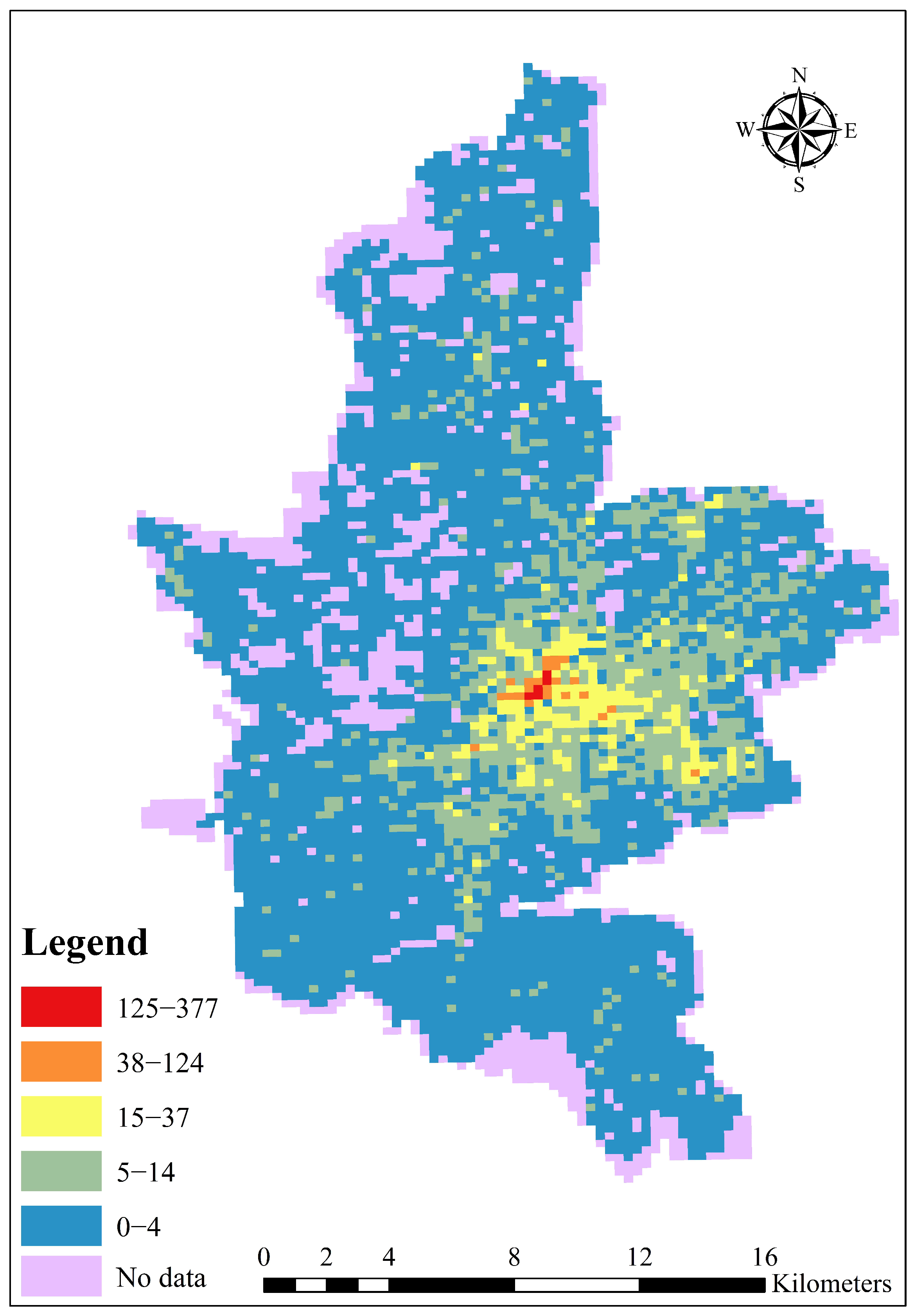
Figure A1 and Table A1 show the score for amenity accessibility. The DeepLab V3+ neural network was used to extract the landscape elements. Figure A2 and Table A2 show the landscape elements within the 250 m chunks, regarding greenery, open sky, eye-level building, and eye-level road. The number of pedestrians was determined using the Faster-RCNN neural network target detection. The chunk values were obtained by adding the statistics. Figure 5 shows that the unit values were obtained by adding the statistics.

5.1. Detection of Built Environmental Features Based on OLS Regressions and SLM Regressions

OLS regression was used to conduct an analysis of the built environment features. We verified the built environment’s impact on the pedestrian volume using OLS regression. Table 4 shows the result of seven OLS regressions.
In the city, five built environment features impacted pedestrian volume. Eye-level buildings, the number of intersections, the number of train stations per unit area, the number of bus stops per unit area, entertainment facility, and fitness facility positively affected pedestrian volume. Residential units, open sky, greenery, land use entropy, and distance to city center, had a negative impact on pedestrian volume. The three most influential factors were the number of train stations per unit area (0.082), eye-level buildings (0.071), and the number of intersections per unit area (0.057). In the CC (city center), the number of intersections was a positive influence, and population density and land use entropy were the negative influences. In the LOH (local hub), the number of bus stops per unit area, the number of intersections, eye-level roads, population density, library, school, train stations per unit area, and entertainment facility were positive influences. Distance to city center and grocery were negative influences. The three most influential factors were the population density (0.194), eye-level roads (0.038), and the number of intersections per unit area (0.030). In the LIH (living hub), the number of bus stops per unit area, population density, the number of intersections, land use entropy, and library were positive influences. Distance to the city center was a negative influence. The three most influential factors were the number of intersections (0.025), population density (0.024), and the number of bus stops per unit area (0.018).
In the UPA, the number of intersections (0.018), restaurants (0.009), and the number of bus stops per unit area (0.005) positively affected pedestrian volume. In the UCA, library, grocery, and entertainment facility had a negative effect. The three most influential factors were the number of intersections (0.021), residential units (0.010), and the number of bus stops per unit area (0.004). In the NPA, the features influencing pedestrian volume contained three dimensions: density, distance to transit (number of bus stops per unit area), and design (the number of intersections), which all had positive effects.
Considering the effects of spatial autocorrelation on pedestrians, we used SLM regression to analyze seven data sets. SLM regression outperformed OLS regression, as shown in Table 5.
In the city, the effect of land use entropy was not significant. The number of train stations, eye-level buildings, and the number of intersections, population density, and residential units negatively affected pedestrian volume. In the CC, the performance was consistent with OLS, with the number of intersections positively correlated and population density and land use entropy negatively correlated. In the LOH, the largest coefficient was eye-level roads (0.037). Intersections, the number of bus stops, the number of train stations, population density, library, and school were positively correlated. Distance to city center was negatively correlated. In the LIH, the number of intersections, population density, the number of bus stops, land use entropy, and library were positively correlated. Distance to city center was negatively correlated. In UPA, intersections, the number of bus stops, and land use entropy were positively correlated. In UCA, the number of intersections, residential units, number of bus stops, and land use entropy were positively correlated with pedestrian volume. However, library, entertainment facility, and grocery, were negatively correlated. Additionally, restaurants positively affected pedestrian volume. In NPA, only population density, intersection density, and the number of bus stops had any effects.

5.2. Detection of Built Environmental Factors Based on Geodetectors

Due to the overall R-square of SLM being higher than the OLS regressions, we used the results of SLM for further analysis. The factors that were significantly correlated were selected. According to the order of most minor to most significant values, independent variables were classified into five subareas by the Jenk’s breaks classification. Geodetector was used to measure the interaction between different built environment features; firstly, using factor detectors, with the results shown in Table 6.
The three factors, which were significant and had the strongest q-values within each model, were selected as the single dominant factor. Then, we used risk detectors to detect subarea heterogeneity for three single dominant factors. In the city, the dominant factors were the eye-level buildings (0.174), the number of intersections (0.125), and the population density (0.114). In the CC, none of the independent variables were significant in the factor detector. In the LOH, the dominant factors were the distance to city center (0.221), the population density (0.190), and the number of bus stops per unit area (0.175). In the LIH, the dominant factors were population density (0.184), the number of intersections (0.173), and the number of bus stops per unit area (0.142). In the UPA, the dominant factors were the number of intersections (0.188), land use entropy (0.095), and the number of bus stops (0.084). In the NPA, the dominant factors were population density (0.469), the number of intersections (0.364), and the number of bus stops per unit area (0.296).
Secondly, we explored the interaction between factors within each functional area with the help of interaction detectors, and selected the three interaction factors with the strongest q-values as the dominant interaction factors. However, in the CC, based on its single-factor significance, we could not obtain the interaction. Table 7 shows the results of dominant interaction factors.
In the city, the differences in the number of bus stops per unit area and residential units were not significant. Additionally, the spatial differences between the other factors were significant. Residential units and the number of intersections differed insignificantly in subarea four and subarea five. The number of bus stops differed insignificantly in subarea three and subarea two. The areas with high public transportation and high residential density had more walkers. In the LOH, the spatial differences between distance to city center and population density, eye-level roads, and the number of bus stops per unit area were not significant. Additionally, the spatial differences were obvious in the subareas of the distance to city center. In the LIH, there is no spatially significant difference between population density, intersection density, and library. Library and the number of intersections were not significantly different. Among the subareas of library, only subarea one differed significantly from the other subareas, and the other subareas were not significantly different. In the UPA, there is no significant difference between land use entropy and the number of intersections or land use entropy and the number of bus stops. The differences between subareas for land use entropy and the number of intersections were significant. In the UCA, the spatial differences for residential units, land use entropy, and the number of intersections were not significant. Spatial differences were significant for residential units and land use entropy. The spatial differences of the number of intersections between subarea five and other subareas were insignificant. In the NPA, the spatial differences between the number of intersections and the number of bus stops per unit area were not significant.

6. Discussion

This study extends the research on the spatial differences of built environment impact on population-level walking behavior (pedestrian volume) within different functional areas. First, it confirmed the differences for the effects of built environment factors on pedestrian volume within different functional areas. Second, the effects of built environment interaction were supplemented by walkability research. This study systematically explored pedestrian volume and the built environments of compact cities. The results are beneficial for advancing research on related topics, such as walkable cities, healthy cities, and urban planning.
The study explored the effect of built environment features on pedestrian volume by constructing seven models and using regression and Geodetector. The results of the study are as follows. Firstly, the impact of land use entropy was insignificant over the entire city. Eye-level buildings, population density, and the number of intersections were dominant factors. In addition, distance to transit was positively correlated and mentioned in the design of walkable cities [17]. Intersections were a positive correlation which is also confirmed in previous studies [14,15,41]. The spatial differences in residential units and the number of intersections were not significant. The bus stops interacted with population density or intersections and dominated pedestrian volume at the whole city level. However, the population density negatively affected pedestrian volume in this study. The population density data was statistical, representing a residential density. Collective walking behaviors [36] usually occur in commercial areas of the city. The higher eye-level buildings were generally in the commercial center area of the city center or in the local hubs, and pedestrians tended toward commercial spaces. Therefore, the eye-level buildings had a dominant effect on the spatial distribution of the pedestrians, which was positive.
In the city center, design, density, and diversity affected pedestrian volume (in the city center), which was proposed in the theory of the 3 Ds [15]. Previous studies in Japan confirmed that residential density, land use diversity, good infrastructure, and street aesthetics are positively correlated with walking activities [42]. The positive correlation between population density and walking was confirmed [43]. However, in this study, diversity and population density negatively affected pedestrian volume in the city center. High-density population areas [44] and high land use mixtures [45] in non-residential areas did not promote walking activity. Peoples’ walking was concentrated in commercial areas, so diversity was negatively correlated. Additionally, the number of intersections positively correlates with pedestrian volume, as in previous studies [4,17].
In the local hub, the distance to the city center, population density, and the number of bus stops mainly dominated pedestrian volume. Distance to the city center negatively affected pedestrian volume. The number of bus stops, intersections, and population density were positively correlated with pedestrian volume, as mentioned in previous studies [4,14]. An increase in the density of transportation services was associated with increased pedestrian volume [43]. People were more likely to be walkers if they lived in an area with a well-connected street network and convenient train stations [46]. In addition, school and library promoted pedestrian volume in the local hub. The eye-level roads were good for walking. This finding was similar to that of Kim et al. [47], who found that the relationship between pedestrian volume and street width changes.
In the living hub, population density, the number of intersections, and the number of bus stops dominated the pedestrian volume. The influence of density, the number of intersections, and the distance to transit were positive for pedestrian volume. But residents outside the range of the transit station were relatively less likely to walk for leisure [48]. The impact of local accessibility was not as strong as the local hub. High-density residential density negatively affected peoples’ walking time [49], but in Kumamoto City, most of the buildings are two-story residential buildings. Therefore, density positively affected pedestrian volume. Intersections did not have spatial differences with population density and library. Their interactions were powerful. The interaction between population density and the number of bus stops dominated pedestrian volume.
In the UPA, land use entropy, the number of intersections, and bus stops dominated pedestrian volume, and all were positively correlated. In low-population density areas, population density and walking were positively correlated [44], and diversity had a positive effect on walking, as in previous studies [50,51]. The strongest interaction was the number of intersections and the number of bus stops per unit area. The spatial differences were insignificant within land use entropy and the number of intersections, or land use entropy and the number of bus stops per unit area. In sparsely populated areas, any physical environment associated with walking would promote walking behavior [52].
In the UCA, residential units, land use entropy, and the number of intersections dominated pedestrian volume. The number of intersections had the largest effect and was positively correlated. Local accessibility to library, restaurants, and grocery impacted pedestrian volume, but their impacts were not particularly strong. Destination accessibility and walking were correlated. Increasing destinations could increase adults walking activity for transport-related walking, but there was no effect on leisure walking [53]. The interactions among residential units, the number of intersections, and land use entropy dominated pedestrian volume. Additionally, the spatial differences between them were not significant. In the NPA, population density, the number of intersections, and the number of bus stops per unit area dominated pedestrian volume. The population density was the most vital factor affecting pedestrian volume.
Based on the above findings, we reveal the differences in the impact of the built environment on different functional areas, city centers (diversity, design, and density), local hubs (destination accessibility, density, distance to transit), living hubs (density, design, and distance to transit), UPA (diversity, design, and distance to transit), UCA (density, density, and design), and NPA (density). Design and density, at the whole city level, significantly impacted pedestrian volume. Additionally, the population density and the land use diversity in the overly dense population area were negatively related to pedestrian volume.
This study had the following limitations. Due to the study using 250 m chunks, the number of grids was not the same when analyzing different functional areas, which affects the analysis results in those functional areas that had fewer grids. Second, owing to data limitations, the age and physical condition of pedestrians cannot be analyzed; therefore, this study cannot clearly define the relationship between personal factors and pedestrian volume. Thirdly, some aspects of street design in different functional areas, such as road comfort, road safety, and aesthetics, were not explored.
7. Conclusions

This study analyzes the influence of built environment features on pedestrian volume in different functional urban areas. We used regression and Geodetector to discuss the relationship between built environment factors and pedestrian volume. It was found that urban area design and density significantly impacted pedestrian volume over the entire city. Different built environment features affected pedestrian volume in various functional urban areas, including the city centers (diversity, design, and density), local hubs (destination accessibility, density, and distance to transit), living hubs (density, design, and distance to transit), UPA (diversity, design, and distance to transit), UCA (density, density, and design), and NPA (density). Additionally, population density and land use diversity in the overly dense population areas were negatively related to pedestrian volume. Therefore, governments and urban planners need to propose different improvement options for different functional areas to promote walkability and improve the built environment.

Author Contributions

C.F. and R.H.: conceptualization, methodology; C.F.: investigation, software, data curation, writing—original draft preparation; C.F., R.H., Q.L., H.L. and A.S.S.R.: writing—review and editing, validation; C.F. and R.H.: supervision, project administration. All authors have read and agreed to the published version of the manuscript.

Funding

This research received no external funding.

Institutional Review Board Statement

Not applicable.

Informed Consent Statement

Not applicable.

Data Availability Statement

The datasets in this study are publicly available and detailed in Section 3.

Acknowledgments

The support provided by the China Scholarship Council (CSC No.202108050061) and the Riken Homma laboratory, Graduate School of Science and Technology, Kumamoto University.

Conflicts of Interest

The authors declare no conflict of interest.

Appendix A

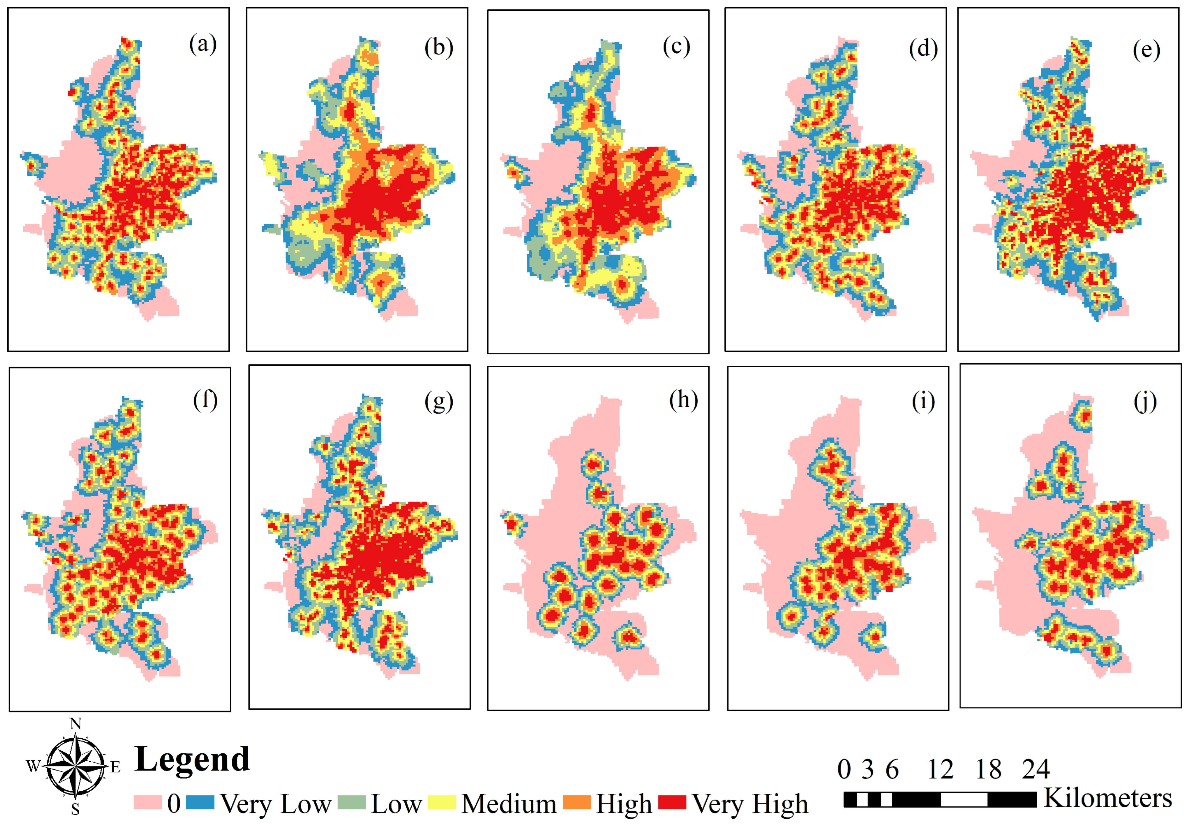
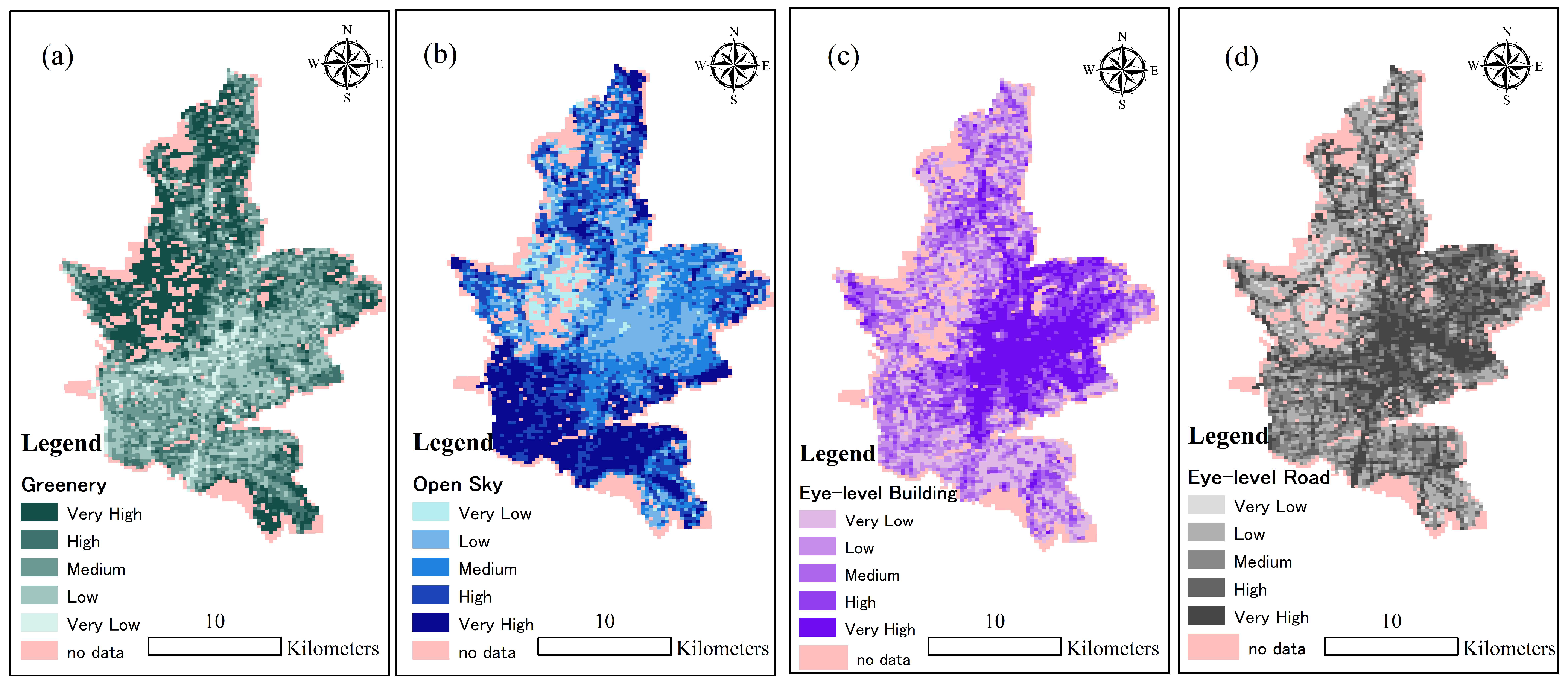
The scores for amenity accessibility or the statistics of the landscape elements are divided into five categories from low to high by quantile classification, as shown in Figure A1 and Figure A2.
Figure A1. Amenity accessibility: (a) grocery; (b) restaurants; (c) shopping; (d) bank; (e) park; (f) school; (g) hospital; (h) library; (i) fitness facility; (j) entertainment facility.
Sustainability 14 11636 g0a1
The scores for amenity accessibility are shown in Figure A1 and Table A1; the amenity accessibility score in the UCA and NPA was lower than the Kumamoto City average score, whereas the areas within the UPA were higher than the Kumamoto City average score. Furthermore, after leaving the UPA, the scores for parks and groceries began to rapidly decline, while the accessibility to libraries within the UCA rapidly declined when moving away from the city center. The score for entertainment facilities dropped away sharply from the city center, but the scores between the local hub and living hub remained relatively stable.
Table A1. The average score of amenity accessibility in different function area.
City CenterLocal HubLiving HubUPAUCANPAKumamoto City
Grocery98.32294.03294.98576.66536.3426.22551.233
Restaurants99.59692.75088.08265.35818.8359.06739.082
Shopping98.65393.40990.90470.53120.9306.76541.101
Bank99.19594.91287.82769.46935.08724.18850.475
Park99.73397.93197.34493.83449.1432.15961.194
School94.88287.22479.07663.35728.77017.45643.809
Hospital99.67498.37697.60383.81337.45227.44155.258
Library63.99550.91237.62920.1515.1726.12215.612
Fitness facility88.25173.23361.76738.8228.5560.00024.331
Entertainment facility91.72766.94660.72935.44210.4223.05124.533
Figure A2 and Table A2 show that an increase in distance from the city center correlates with a gradual increase in greenery and open sky. However, in the NPA, the open sky decreased, whereas the greenery increased. This was because of the presence of forests and tall trees in the NPA. Furthermore, because the UCA has substantial cropland, there is an extremely high presence of open sky. The functional areas from the city center to the NPA, are the eye-level buildings and eye-level roads. In areas far from the city center, eye-level roads take on distinct lines in their spatial distribution. In addition, eye-level buildings decreased faster than the eye-level roads.
Table A2. The average ratio of statistics for landscape elements.
City CenterLocal HubLiving HubUPAUCANPAKumamoto City
Greenery10.965%11.841%13.553%16.451%18.563%28.102%17.828%
Open sky16.883%24.476%23.896%26.446%26.659%15.385%25.100%
Eye-level roads33.611%30.020%29.450%26.841%20.087%15.720%22.661%
Eye-level buildings30.240%22.266%21.120%14.554%5.140%5.346%9.931%
Figure A2. Statistics of landscape elements: (a) greenery; (b) open sky; (c) eye-level building; (d) eye-level road.
Sustainability 14 11636 g0a2

References

  1. Ministry of Land, Infrastructure, Transport and Tourism. Creating a Town for Walk Comfortably-Forming a Walkable Town-. Available online: https://www.mlit.go.jp/toshi/toshi_machi_tk_000072.html (accessed on 24 June 2022).
  2. Kumamoto Metropolitan Area Traffic Planning Council. Kumamoto Metropolitan Area Urban Transportation Master Plan. Available online: https://www.pref.kumamoto.jp/soshiki/103/1303.html (accessed on 20 June 2022).
  3. Burden, D.; Davis, D.; Sprowls, S.; Zykofsky, P.; Wallwork, M. Street Design Guidelines for Healthy Neighborhoods; Center for Livable Communities: Sacramento, CA, USA, 1999. [Google Scholar]
  4. Chen, L.; Lu, Y.; Ye, Y.; Xiao, Y.; Yang, L. Examining the association between the built environment and pedestrian volume using street view images. Cities 2022, 127, 103734. [Google Scholar] [CrossRef]
  5. Booth, M.L.; Bauman, A.; Owen, N.; Gore, C.J. Physical Activity Preferences, Preferred Sources of Assistance, and Perceived Barriers to Increased Activity among Physically Inactive Australians. Prev. Med. 1997, 26, 131–137. [Google Scholar] [CrossRef]
  6. Giles-Corti, B.; Vernez-Moudon, A.; Reis, R.; Turrell, G.; Dannenberg, A.L.; Badland, H.; Foster, S.; Lowe, M.; Sallis, J.F.; Stevenson, M.; et al. City planning and population health: A global challenge. Lancet 2016, 388, 2912–2924. [Google Scholar] [CrossRef]
  7. Murtagh, E.M.; Nichols, L.; Mohammed, M.A.; Holder, R.; Nevill, A.; Murphy, M.H. The effect of walking on risk factors for cardiovascular disease: An updated systematic review and meta-analysis of randomised control trials. Prev. Med. 2015, 72, 34–43. [Google Scholar] [CrossRef]
  8. Bailey, D.P.; Locke, C.D. Breaking up prolonged sitting with light-intensity walking improves postprandial glycemia, but breaking up sitting with standing does not. J. Sci. Med. Sport 2015, 18, 294–298. [Google Scholar] [CrossRef] [PubMed]
  9. Hall, K.S.; Hyde, E.T.; Bassett, D.R.; Carlson, S.A.; Carnethon, M.R.; Ekelund, U.; Evenson, K.R.; Galuska, D.A.; Kraus, W.E.; Lee, I.-M.; et al. Systematic review of the prospective association of daily step counts with risk of mortality, cardiovascular disease, and dysglycemia. Int. J. Behav. Nutr. Phys. Act. 2020, 17, 78. [Google Scholar] [CrossRef] [PubMed]
  10. Keall, M.D.; Shaw, C.; Chapman, R.; Howden-Chapman, P. Reductions in carbon dioxide emissions from an intervention to promote cycling and walking: A case study from New Zealand. Transp. Res. Part D Transp. Environ. 2018, 65, 687–696. [Google Scholar] [CrossRef]
  11. Neves, A.; Brand, C. Assessing the potential for carbon emissions savings from replacing short car trips with walking and cycling using a mixed GPS-travel diary approach. Transp. Res. Part A Policy Pr. 2018, 123, 130–146. [Google Scholar] [CrossRef]
  12. de Nazelle, A.; Morton, B.J.; Jerrett, M.; Crawford-Brown, D. Short trips: An opportunity for reducing mobile-source emissions? Transp. Res. Part D Transp. Environ. 2010, 15, 451–457. [Google Scholar] [CrossRef]
  13. Wang, J.-F.; Li, X.-H.; Christakos, G.; Liao, Y.-L.; Zhang, T.; Gu, X.; Zheng, X.-Y. Geographical detectors-based health risk assessment and its application in the neural tube defects study of the Heshun region, China. Int. J. Geogr. Inf. Sci. 2010, 24, 107–127. [Google Scholar] [CrossRef]
  14. Ewing, R.; Cervero, R. Travel and the Built Environment. J. Am. Plan. Assoc. 2010, 76, 265–294. [Google Scholar] [CrossRef]
  15. Cervero, R.; Kockelman, K. Travel demand and the 3Ds: Density, diversity, and design. Transp. Res. Part D Transp. Environ. 1997, 2, 199–219. [Google Scholar] [CrossRef]
  16. Lee, C.; Moudon, A.V. The 3Ds+R: Quantifying land use and urban form correlates of walking. Transp. Res. Part D Transp. Environ. 2006, 11, 204–215. [Google Scholar] [CrossRef]
  17. Southworth, M. Designing the Walkable City. J. Urban Plan. Dev. 2005, 131, 246–257. [Google Scholar] [CrossRef]
  18. Jacobs, J. The Death and Life of Great American Cities; Random House: New York, NY, USA, 1961. [Google Scholar]
  19. Saelens, B.E.; Sallis, J.F.; Frank, L.D. Environmental correlates of walking and cycling: Findings from the transportation, urban design, and planning literatures. Ann. Behav. Med. 2003, 25, 80–91. [Google Scholar] [CrossRef]
  20. Frank, L.D.; Schmid, T.L.; Sallis, J.F.; Chapman, J.; Saelens, B.E. Linking objectively measured physical activity with objectively measured urban form: Findings from SMARTRAQ. Am. J. Prev. Med. 2005, 28, 117–125. [Google Scholar] [CrossRef]
  21. Frank, L.D.; Sallis, J.F.; Saelens, B.E.; Leary, L.; Cain, K.; Conway, T.L.; Hess, P.M. The development of a walkability index: Application to the Neighborhood Quality of Life Study. Br. J. Sports Med. 2010, 44, 924–933. [Google Scholar] [CrossRef]
  22. Carr, L.J.; Dunsiger, S.I.; Marcus, B.H. Validation of Walk Score for estimating access to walkable amenities. Br. J. Sports Med. 2011, 45, 1144–1148. [Google Scholar] [CrossRef]
  23. Walk Score. Walk Score Methodology. Available online: https://www.walkscore.com/methodology.shtml (accessed on 24 June 2022).
  24. Hino, K.; Baba, H.; Kim, H.; Shimizu, C. Validation of a Japanese walkability index using large-scale step count data of Yokohama citizens. Cities 2022, 123, 103614. [Google Scholar] [CrossRef]
  25. Koohsari, M.J.; Sugiyama, T.; Hanibuchi, T.; Shibata, A.; Ishii, K.; Liao, Y.; Oka, K. Validity of Walk Score(R) as a measure of neighborhood walkability in Japan. Prev. Med. Rep. 2018, 9, 114–117. [Google Scholar] [CrossRef]
  26. Kato, H.; Kanki, K. Development of Walkability Indicator for Smart Shrinking. Int. Rev. Spat. Plan. Sustain. Dev. 2020, 8, 39–58. [Google Scholar] [CrossRef]
  27. Kim, S.; Park, S.; Lee, J.S. Meso- or micro-scale? Environmental factors influencing pedestrian satisfaction. Transp. Res. Part D Transp. Environ. 2014, 30, 10–20. [Google Scholar] [CrossRef]
  28. Lu, Y.; Sarkar, C.; Xiao, Y. The effect of street-level greenery on walking behavior: Evidence from Hong Kong. Soc. Sci. Med. 2018, 208, 41–49. [Google Scholar] [CrossRef] [PubMed]
  29. Nagata, S.; Nakaya, T.; Hanibuchi, T.; Amagasa, S.; Kikuchi, H.; Inoue, S. Objective scoring of streetscape walkability related to leisure walking: Statistical modeling approach with semantic segmentation of Google Street View images. Health Place 2020, 66, 102428. [Google Scholar] [CrossRef]
  30. Zhou, H.; He, S.; Cai, Y.; Wang, M.; Su, S. Social inequalities in neighborhood visual walkability: Using street view imagery and deep learning technologies to facilitate healthy city planning. Sustain. Cities Soc. 2019, 50, 101605. [Google Scholar] [CrossRef]
  31. Lee, S.; Yoo, C.; Seo, K.W. Determinant Factors of Pedestrian Volume in Different Land-Use Zones: Combining Space Syntax Metrics with GIS-Based Built-Environment Measures. Sustainability 2020, 12, 8647. [Google Scholar] [CrossRef]
  32. Ewing, R.; Clemente, O.; Neckerman, K.M.; Purciel-Hill, M.; Quinn, J.W.; Rundle, A. Measuring Urban Design: Metrics for Livable Places; Springer: Berlin/Heidelberg, Germany, 2013; Volume 200. [Google Scholar]
  33. Hajrasouliha, A.; Yin, L. The impact of street network connectivity on pedestrian volume. Urban Stud. 2014, 52, 2483–2497. [Google Scholar] [CrossRef]
  34. Yin, L.; Cheng, Q.; Wang, Z.; Shao, Z. ‘Big data’ for pedestrian volume: Exploring the use of Google Street View images for pedestrian counts. Appl. Geogr. 2015, 63, 337–345. [Google Scholar] [CrossRef]
  35. Chen, L.; Lu, Y.; Sheng, Q.; Ye, Y.; Wang, R.; Liu, Y. Estimating pedestrian volume using Street View images: A large-scale validation test. Comput. Environ. Urban Syst. 2020, 81, 101481. [Google Scholar] [CrossRef]
  36. Jiang, Y.; Chen, L.; Grekousis, G.; Xiao, Y.; Ye, Y.; Lu, Y. Spatial disparity of individual and collective walking behaviors: A new theoretical framework. Transp. Res. Part D Transp. Environ. 2021, 101, 103096. [Google Scholar] [CrossRef]
  37. Urban Policy Division, U.C.B., Kumamoto City Office. Creating a Compact Community with Effective Public Transport. Available online: https://www.city.kumamoto.jp/hpKiji/pub/detail.aspx?c_id=5&id=9398&e_id=9 (accessed on 7 July 2022).
  38. Liu, H.; Homma, R.; Liu, Q.; Fang, C. Multi-Scenario Prediction of Intra-Urban Land Use Change Using a Cellular Automata-Random Forest Model. ISPRS Int. J. Geo-Inf. 2021, 10, 503. [Google Scholar] [CrossRef]
  39. Chen, L.-C.; Zhu, Y.; Papandreou, G.; Schroff, F.; Adam, H. Encoder-Decoder with Atrous Separable Convolution for Semantic Image Segmentation. In Proceedings of the European Conference on Computer Vision (ECCV), Munich, Germany, 8–14 September 2018; pp. 801–818. [Google Scholar]
  40. Ren, S.; He, K.; Girshick, R.; Sun, J. Faster R-CNN: Towards Real-Time Object Detection with Region Proposal Networks. IEEE Trans. Pattern Anal. Mach. Intell. 2016, 39, 1137–1149. [Google Scholar] [CrossRef] [PubMed]
  41. Saelens, B.E.; Handy, S.L. Built environment correlates of walking: A review. Med. Sci. Sports Exerc. 2008, 40 (Suppl. 7), S550–S566. [Google Scholar] [CrossRef]
  42. Inoue, S.; Ohya, Y.; Odagiri, Y.; Takamiya, T.; Ishii, K.; Kitabayashi, M.; Suijo, K.; Sallis, J.F.; Shimomitsu, T. Association between Perceived Neighborhood Environment and Walking among Adults in 4 Cities in Japan. J. Epidemiol. 2010, 20, 277–286. [Google Scholar] [CrossRef] [PubMed]
  43. Joh, K.; Chakrabarti, S.; Boarnet, M.G.; Woo, A. The Walking Renaissance: A Longitudinal Analysis of Walking Travel in the Greater Los Angeles Area, USA. Sustainability 2015, 7, 8985–9011. [Google Scholar] [CrossRef]
  44. Lu, Y.; Xiao, Y.; Ye, Y. Urban density, diversity and design: Is more always better for walking? A study from Hong Kong. Prev. Med. 2017, 103, S99–S103. [Google Scholar] [CrossRef]
  45. Sung, H.; Lee, S. Residential built environment and walking activity: Empirical evidence of Jane Jacobs’ urban vitality. Transp. Res. Part D Transp. Environ. 2015, 41, 318–329. [Google Scholar] [CrossRef]
  46. Kamruzzaman, M.; Washington, S.; Baker, D.; Brown, W.; Giles-Corti, B.; Turrell, G. Built environment impacts on walking for transport in Brisbane, Australia. Transportation 2014, 43, 53–77. [Google Scholar] [CrossRef]
  47. Kim, T.; Sohn, D.-W.; Choo, S. An analysis of the relationship between pedestrian traffic volumes and built environment around metro stations in Seoul. KSCE J. Civ. Eng. 2016, 21, 1443–1452. [Google Scholar] [CrossRef]
  48. Lu, Y.; Gou, Z.; Xiao, Y.; Sarkar, C.; Zacharias, J. Do Transit-Oriented Developments (TODs) and Established Urban Neighborhoods Have Similar Walking Levels in Hong Kong? Int. J. Environ. Res. Public Health 2018, 15, 555. [Google Scholar] [CrossRef] [Green Version]
  49. Qin, Z.; Wang, Z.; Ye, Q.; Jia, P.; Xiong, Y.; Xu, F. Relation between residential density and walking time among urban adults in Nanjing, China. Public Health 2020, 181, 34–39. [Google Scholar] [CrossRef] [PubMed]
  50. Rodriguez, D.A.; Evenson, K.R.; Diez Roux, A.V.; Brines, S.J. Land use, residential density, and walking. The multi-ethnic study of atherosclerosis. Am. J. Prev. Med. 2009, 37, 397–404. [Google Scholar] [CrossRef] [PubMed]
  51. McCormack, G.R.; Giles-Corti, B.; Bulsara, M. The relationship between destination proximity, destination mix and physical activity behaviors. Prev. Med. 2008, 46, 33–40. [Google Scholar] [CrossRef] [PubMed]
  52. Brüchert, T.; Hasselder, P.; Quentin, P.; Bolte, G. Walking for Transport among Older Adults: A Cross-Sectional Study on the Role of the Built Environment in Less Densely Populated Areas in Northern Germany. Int. J. Environ. Res. Public Health 2020, 17, 9479. [Google Scholar] [CrossRef] [PubMed]
  53. Barton, H.; Grant, M.; Guise, R. Shaping Neighbourhoods: For Local Health and Global Sustainability; Routledge: London, UK, 2006. [Google Scholar]
Figure 1. The research area: (a) the image of compact city planning and (b) the functional areas.
Sustainability 14 11636 g001
Figure 2. The built environment features: (a) population density; (b) residential units; (c) land use entropy; (d) intersections; (e) train stations; (f) bus stops.
Sustainability 14 11636 g002
Figure 3. Structure of DeepLab v3+ neural network.
Sustainability 14 11636 g003
Figure 4. Structure of Faster-RCNN neural network.
Sustainability 14 11636 g004
Figure 5. Statistics of pedestrian volume detection (the number of pedestrians).
Sustainability 14 11636 g005
Table 1. Research data and sources.
CategoryDimensionsInfluencing FactorsData Source
Independent variable (built environment)DensityPopulation density2015 census data from e-stat
Residential units2017 Kumamoto City Basic Survey
DiversityLand use entropy2017 Kumamoto City Basic Survey
DesignThe number of intersections per unit areaOpen Street Map (OSM)
Greenery; open sky; eye-level building; eye-level roadStreet-view images of Google Maps (www.google.com/maps, accessed on 24 July 2022)
Destination accessibilityRegional accessibility (distance to city center)2017 Kumamoto City Basic Survey
Local accessibility (grocery; restaurants; shopping; bank; fitness facility; entertainment facility)MapFan website (mapfan.com, accessed on 24 July 2022, in Japanese) in 2022
Local accessibility (park; school; hospital; library)the Ministry of Land, Infrastructure, Transport, and Tourism (nlftp.mlit.go.jp/ksj/, accessed on 24 July 2022)
Distance to transitThe number of train stations per unit area
The number of bus stops per unit area
2017 Kumamoto City Basic Survey
Dependent variablePedestrian volumeThe number of pedestrians per unit areaStreet-view images of Google Maps
Table 2. Category of amenities.
CategorySubcategories
GroceryConvenience stores
RestaurantsRestaurant, izakaya, Chinese restaurant, sushi restaurant, etc.
ShoppingShopping mall, department store, supermarket, clothing store, home appliance store, and second-hand market.
BankJapan post bank, Higo bank, Kumamoto bank, etc.
ParkPark
SchoolUniversity, high school, middle school, elementary school
HospitalHospital
LibraryLibrary
Fitness facilityStadium, gymnasium
Entertainment facilityKaraoke, theater, game center, pet rides
Table 3. Interaction between built environment factors.
Judgment StandardInteraction Type
q(x1 ∩ x2) < Min(q(x1), q(x2))Weaken, nonlinear
Min(q(x1), q(x2)) < q(x1 ∩ x2) < Max(q(x1), q(x2))Weaken, univariate
q(x1 ∩ x2) > Max(q(x1), q(x2))Enhance, bivariate
q(x1 ∩ x2) = q(x1) + q(x2)Independent
q(x1 ∩ x2) > q(x1) + q(x2)Enhance, nonlinear
Table 4. Result of OLS regression in different functional areas.
Explanatory FactorCityCCLOHLIHUPAUCANPA
Population density−0.002−0.329 **0.194 **0.024 ***0.0010.0040.054 **
Residential units−0.043 ***−0.270−0.0070.0000.0010.010 ***0.001
Land use entropy−0.005 *−0.509 ***0.0020.015 **0.0040.002 *−0.01
The number of intersections0.057 ***0.636 ***0.030 ***0.025 ***0.018 ***0.021 ***0.018 **
Greenery−0.031 **0.408−0.006−0.004−0.011−0.043−0.005
Open sky−0.023 **0.402−0.009−0.001−0.008−0.003−0.003
Eye-level buildings0.071 ***1.4360.0290.0160.0020.004−0.001
Eye-level roads−0.0000.0540.038 *0.0020.0070.000−0.001
Distance to city center−0.004 * −0.026 ***−0.011 **−0.0020.0000.000
Grocery0.0010.038−0.018 *−0.002−0.001−0.001 **0.032
Restaurants−0.003−0.0170.0070.0110.005 *0.001 **−0.002
Shopping−0.004−0.2790.0110.002−0.0020.000−0.001
Bank0.001−0.796−0.013−0.0020.0010.001 *0.000
Park−0.0010.280−0.019−0.0100.0000.001 *−0.002
School0.0000.0250.013 **0.0050.000−0.0000.000
Hospital−0.001−0.445−0.015−0.003−0.0020.000−0.000
Library0.0030.0260.007 ***0.006 **0.001−0.002 ***−0.028
Fitness facility0.004 *0.1200.0030.0010.0020.001 *
Entertainment facility0.005 ***−0.0170.005 *−0.0000.002−0.001 *0.001
The number of train stations per unit area0.082 ***0.0470.018 **−0.006 0.003
The number of bus stops per unit area0.013 ***0.0020.017 ***0.018 ***0.009 ***0.004 ***0.012 ***
Constant0.0230.8310.013−0.0130.0030.0030.004
R-squared0.2800.7720.5010.4300.3440.2490.585
Note: * p < 0.05; ** p < 0.01; *** p < 0.001.
Table 5. Result of SLM regression in different functional areas.
Explanatory FactorCityCCLOHLIHUPAUCANPA
Population density−0.014 **−0.322 **0.011 *0.020 **−0.0010.0050.054 **
Residential units−0.012 ***−0.248−0.0020.0020.0020.010 ***0.001
Land use entropy−0.004−0.507 ***0.0050.016 ***0.005 **0.002 **−0.001
The number of intersections0.031 ***0.617 ***0.026 ***0.020 ***0.017 ***0.020 ***0.018 ***
Greenery−0.0110.439−0.008−0.010−0.010−0.004−0.005
Open sky−0.0060.422−0.007−0.005−0.007−0.003−0.003
Eye-level buildings0.038 ***1.4330.0230.0000.0030.004−0.001
Eye-level roads0.0020.0770.037 *0.0130.0080.001−0.001
Distance to city center0.002 −0.012 *−0.012 *−0.0010.0000.001
Grocery0.0000.020−0.014−0.003−0.001−0.001 *0.033
Restaurants−0.003−0.2280.0020.0090.0050.001 *−0.003
Shopping−0.003−0.2490.003−0.001−0.0020.000−0.001
Bank0.001−0.802−0.007−0.0020.0010.0010.000
Park−0.0000.159−0.012−0.0080.0010.0000.002
School−0.0010.0210.008 *0.0040.000−0.0000.000
Hospital−0.000−0.415−0.009−0.001−0.0020.000−0.001
Library0.0000.0280.005 *0.005 *0.001−0.002 ***−0.029
Fitness facility0.0010.1080.0020.0010.0020.009
Entertainment facility0.0010.0140.003−0.0010.002−0.001 *0.000
The number of train stations per unit area0.051 ***0.0500.016 **−0.005 0.004
The number of bus stops per unit area0.011 ***0.0010.016 ***0.018 ***0.008 ***0.004 ***0.012 ***
Constant0.0040.951−0.0010.2510.0000.0020.004
R-squared0.5570.7680.5570.4600.3600.2520.586
Note: * p < 0.05; ** p < 0.01; *** p < 0.001.
Table 6. Result of q-value from the factor detector of Geodetector.
Explanatory FactorCityCCLOHLIHUPAUCANPA
Population density0.114 ***0.0330.190 ***0.184 *** 0.469 ***
Residential units0.061 *** 0.137 ***
Land use entropy 0.055 0.030 **0.095 ***0.126 ***
The number of intersections0.125 ***0.1490.148 ***0.173 ***0.167 ***0.109 ***0.364 ***
Eye-level buildings0.174 ***
Eye-level roads 0.157 ***
Distance to city center 0.221 ***0.065 ***
Grocery 0.027 ***
Restaurants 0.037 ***
School 0.089 ***
Library 0.044 ***0.111 *** 0.005 *
Entertainment facility 0.004
The number of train stations per unit area0.086 *** 0.052 **
The number of bus stops per unit area0.063 *** 0.175 ***0.142 ***0.084 ***0.055 ***0.296 ***
Note: * p < 0.05; ** p < 0.01; *** p < 0.001.
Table 7. Interaction between explanatory factors of pedestrian volume.
ModeInteraction Factorq-ValueInteraction Type
CityThe number of bus stops per unit area ∩ The number of intersections0.322Enhance, nonlinear
The number of bus stops per unit area ∩ Residential units0.244Enhance, nonlinear
The number of intersections ∩ Residential units0.211Enhance, nonlinear
LOHDistance to city center ∩ The number of bus stops per unit area0.352Enhance, bivariate
Distance to city center ∩ Population density0.350Enhance, bivariate
Distance to city center ∩ Eye-level roads0.340Enhance, bivariate
LIHPopulation density ∩ The number of bus stops per unit area0.315Enhance, bivariate
Population density ∩ The number of intersections0.286Enhance, bivariate
The number of intersections ∩ Library0.283Enhance, bivariate
UPAThe number of intersections ∩ The number of bus stops per unit area0.282Enhance, nonlinear
The number of intersections ∩ Land use entropy0.258Enhance, bivariate
Land use entropy ∩ The number of bus stops per unit area0.173Enhance, bivariate
UCAResidential units ∩ The number of intersections0.212Enhance, bivariate
Land use entropy ∩ The number of intersections0.200Enhance, bivariate
Residential units ∩ Land use entropy0.180Enhance, bivariate
NPAThe number of bus stops per unit area ∩ Population density0.585Enhance, bivariate
The number of bus stops per unit area ∩ The number of intersections0.529Enhance, bivariate
Population density ∩ The number of intersections0.501Enhance, bivariate
Publisher’s Note: MDPI stays neutral with regard to jurisdictional claims in published maps and institutional affiliations.