Multi-Objective Vehicle Routing Problem for Waste Classification and Collection with Sustainable Concerns: The Case of Shanghai City

Abstract

With the promotion of an ecological civilization philosophy and a sustainable development strategy, solid waste classification and collection has become an emerging issue in China. Based on the three dimensions of sustainable development, namely economy, society, and environment, the route optimization model of waste collection and transportation is constructed. In order to solve the model aiming to maximize the benefits of sanitation companies under the constraints of workload balance, transportation cleanliness, and route changes due to cost factors, we combine the non-dominated sorting genetic algorithm III with simulated annealing. According to the characteristics of the problem, the probabilistic insertion method is incorporated to generate the initial solution, and the adaptive mutation operator is added to improve the population diversity. Finally, a real case in Xuhui District, Shanghai, a megacity taking the lead in 2019 in mandating a separated collection policy, is presented to verify the proposed model’s performance. The results provide a decision solution for dispatching the collection route of vehicles with some references for sanitary companies.

1. Introduction

Since entering the 21st century, China’s municipal solid waste output has always been maintained at 100 million tons and presented an increasing trend year by year. The Chinese government introduced several regulations about waste classification (http://www.gov.cn/zhengce/content/2017-03/30/content_5182124.htm (accessed on 15 June 2022)) to protect the environment and save resources. By November 2019, there had been 237 prefecture-level cities in China that began to classify waste, among which Shanghai took the lead in implementing the compulsory waste classification policy [1] and classified the solid waste into wet waste, dry waste, recyclable waste, and hazardous waste [2].

According to the field investigation, the waste collection in Shanghai is mainly undertaken by local sanitation companies in various districts. At the beginning, many wet waste trucks were converted from dry waste ones, inevitably bringing on an adverse impact to the environment, such as exuding unpleasant gas, spreading diseases in high-temperature weather, and causing a leakage problem during transportation [3]. Moreover, implementing classified collection requires more human resources, whereas the personnel of the company does not increase on a large scale. Thus, the existing employees need to take on heavier tasks than before. The employees’ satisfaction will directly influence their motivation to work [4], so balancing the workload of employees has become one of the urgent problems to be solved.

With consideration of the above environmental and workload balancing issues, this paper constructs a vehicle routing optimization model for waste collection and transportation, so as to provide some guidance and suggestions for the practical decision making. To the best of our knowledge, there are relatively few studies that consider both waste leakage and workload balance among employees under the premise of considering the economy. Therefore, it is necessary to conduct more in-depth research for this problem. In addition, China needs to deal with a large amount of domestic waste every year, and the collection and transportation costs account for more than half of the total cost. Therefore, optimizing the vehicle route and personnel allocation of the waste collection system can improve the recycling and utilization efficiency of waste resources, which is of great significance for the construction of resource-saving and environment-friendly cities.

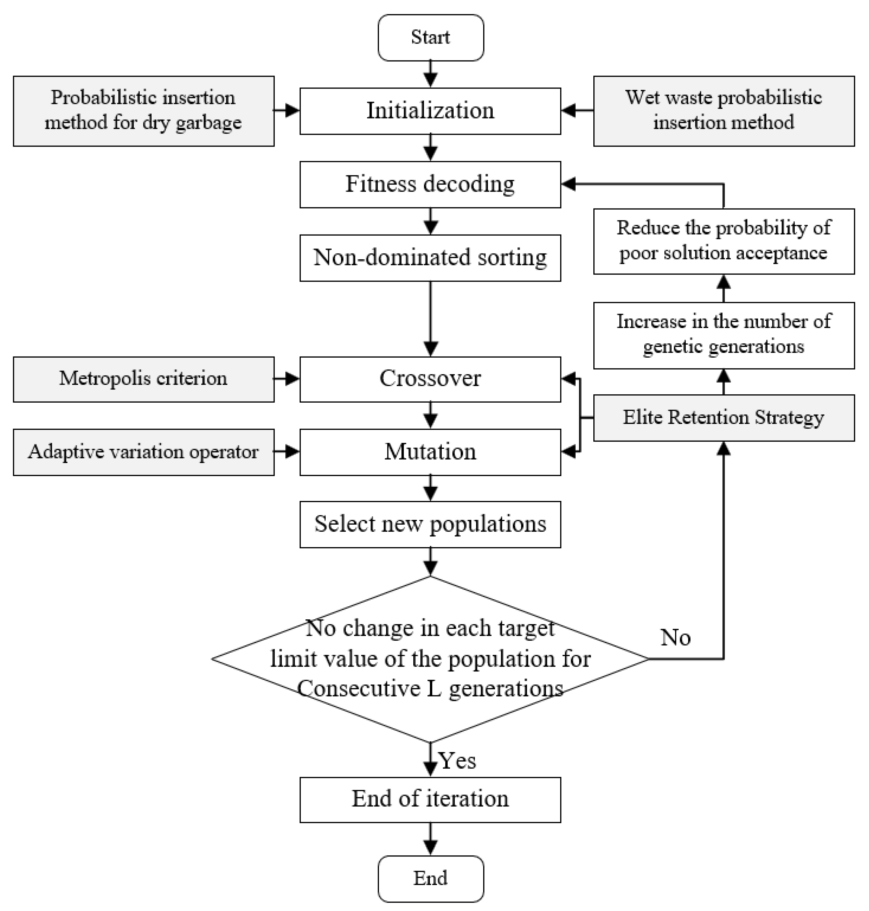
The contributions of this research are as follows: First, from the perspective of practice, taking into account the three factors of sustainable development, the multi-objective vehicle routing optimization model for collecting two kinds of waste is constructed. Second, combining the non-dominated sorting genetic algorithm III (NSGA-III) with the probabilistic insertion method, the Metropolis criterion of the simulated annealing algorithm, and the adaptive mutation operator, an effective improved NSGA-III algorithm is designed. Third, the real case of waste collection in the Xuhui District of Shanghai is carried out, and some management insights are given to propose a comprehensive waste collection program, which can ensure a certain market share and enhance the core competitiveness of the sanitation company.

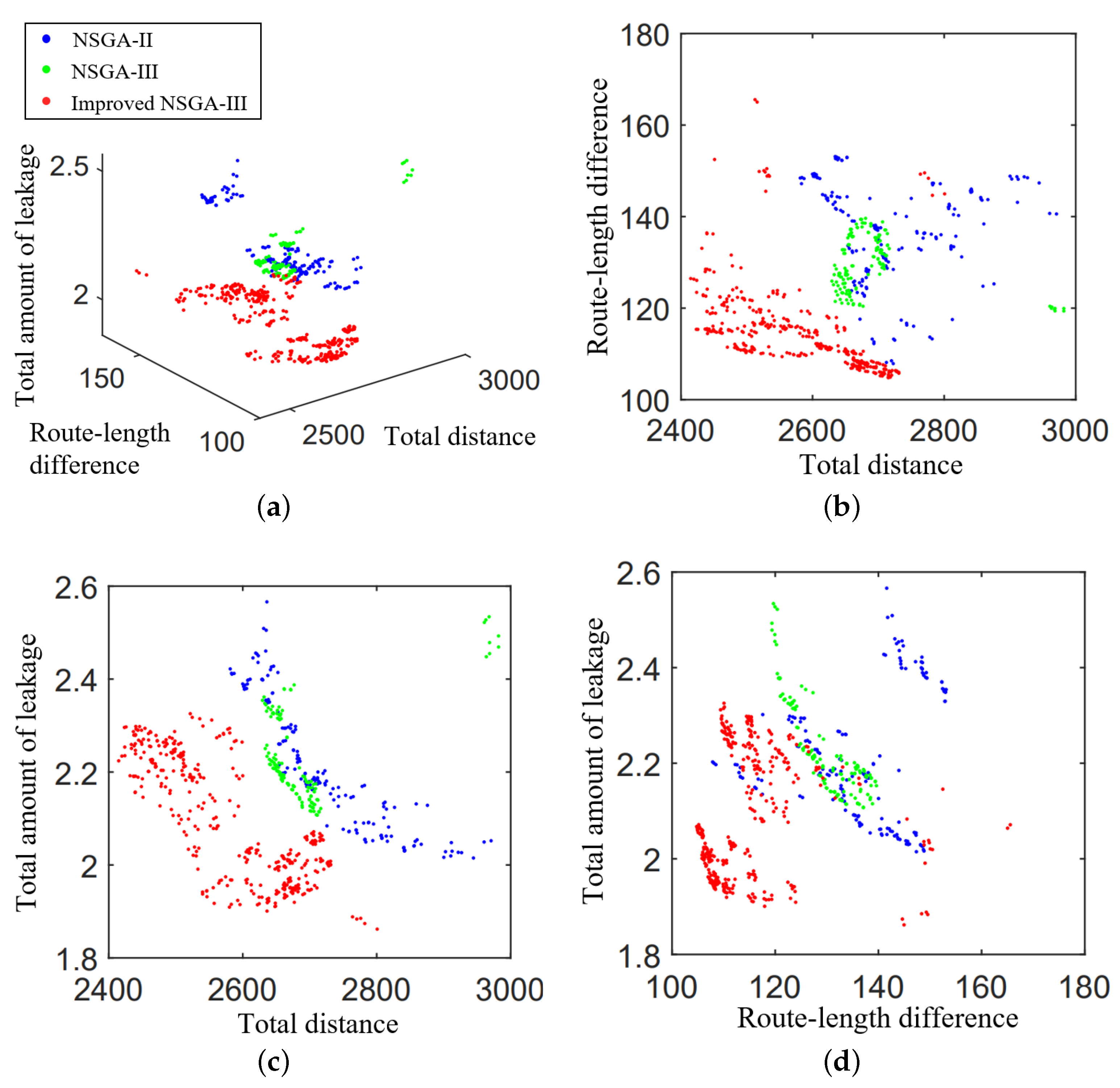
The remainder of this paper is organized as follows. Section 2 reviews the research related to the vehicle routing problem (VRP) with route balancing and reverse logistics. Section 3 presents the mathematical model of the VRP for classified waste collection. Section 4 specifies the improved NASG-III algorithm. Section 5 compares the performance of the proposed algorithm with the non-dominated sorting genetic algorithm II (NSGA-II) and the classic NSGA-III. Section 6 studies the case of Xuhui, Shanghai, and provides some management insights. Section 7 gives the conclusion and future research direction.

2. Literature Review

2.1. VRP in Reverse Logistics

Since the 1990s, the increasing pressure brought by a resource shortage and environmental issues has prompted scholars to focus on the development of reverse logistics. There are four types of reverse logistics networks, i.e., repair, reuse, remanufacture, and recycle, and solid waste collection is one of the main application areas of recycling. Lieckens et al. [5] designed a profit-maximizing stochastic model for a multi-product, multi-level structured network. Vahdani et al. [6] proposed a bi-objective model to design reliable networks for two-way facilities under uncertain conditions. Eskandarpour et al. [7] designed a network, including primary customers, collection/redistribution centers, recycling disposal centers, and secondary customers, in an integrated seven-tier recycling network. Chaabane et al. [8] studied a new reverse logistics routing problem for end-of-life vehicle recycling, combining the classical VRP with the pickup problem and additional constraints (e.g., loading pickup sequences, time windows, multiple trips, heterogeneous internal fleets, and external carriers). Delle et al. [9] proposed a solution strategy based on an integer linear programming model with the aim of improving the efficiency of the allocation of cleaners in urban neighborhoods by determining the leaf bag storage points and routes followed by leaf bag collection vehicles. Delgado-Antequera et al. [10] modeled a real waste collection problem as a VRP with capacity constraints and two objectives: travel cost minimization and routing balancing.

2.2. VRP with Route Balancing

The VRP with route balancing is an extension of the basic VRP, which aims at minimizing the total distance and balancing the workload of employees. Galindres-Guancha et al. [11] proposed a mathematical model, considering both economic and workload balance objectives, and designed an approximation method based on iterative local search metaheuristics and decomposition to solve it. Mancini et al. [12] introduced the collaborative VRP with time consistency, service consistency, and workload balance. Raa et al. [13] proposed a powerful metaheuristic solution which could adequately balance vehicle travel routes, cycle inventory, and various costs. Zhang et al. [14] developed two multi-objective local search algorithms for simultaneously solving the problem of minimizing the total travel cost and balancing the profit of transportation companies. Zhang et al. [15] introduced the model minimizing the maximal routing cost to effectively avoid the occurrence of distortion solutions and developed a multi-objective modal algorithm to obtain the Pareto optimal solution for a VRP with route balancing. In addition, Castaneda et al. [16] proposed a multi-objective approach and an iterative local search metaheuristic to solve the green VRP with private fleets and public carriers. Lehuede et al. [17] studied a lexicographically minimax approach based on the social choice theory and developed a fair model to solve the VRP with route balancing. Janssens et al. [18] constructed a VRP based on region partitioning that allowed minimizing the total distance while balancing the workload of different vehicles and proposed a solution algorithm with a multi-neighborhood forbidden search heuristic to solve this problem. Huang et al. [19] set the maximum allowable workload difference to balance the workload in the periodic routing problem and solved it with the local branching method. Wang and Lin [20] used a two-stage approach in considering the VRP problem with uncertain transportation time, converting various factors into costs, and finally applying real arithmetic examples to test the effect of the approach.

2.3. Green VRP

With the implementation of sustainable development strategies, pollution reduction and environmental protection have become equally topical issues attracting attention when addressing VRPs, and carbon emission is a common indicator measuring environmental impact. Cai et al. [21] investigated a new green VRP arranging connected and automated vehicles to meet customer needs and minimize carbon emissions. Liu and Liao [22] proposed a carbon emission and total cost minimization model, simplified it with k-means clustering, and developed a three-stage method for the solution. Liao [23] proposed formulations and a hybrid metaheuristic algorithm to solve the online VRP minimizing costs related to economics and emissions. Zhang et al. [24] incorporated fuel cost, carbon emission cost, and vehicle usage cost into the traditional VRP and established a low-carbon routing problem model. Considering the distribution cost and carbon emission, Bai et al. [25] proposed a mathematical optimization model and employed the improved NSGA-II algorithm to obtain the Pareto frontal solution set.

Waste management includes waste classification and collection, which itself is with the original intention of environmental protection. In the field of waste collection, Erdem [26] considered multiple types of wastes, optimized waste collection procedures, and transportation operations in a sustainable way and developed an adaptive variable neighborhood search algorithm to solve the electric waste collection problem efficiently. Wu et al. [27] addressed the optimization of urban wet waste collection and transportation in China by combining the carbon emission cost with traditional waste management costs from an environmental perspective. Akhtar et al. [28] presented an improved backtracking search algorithm using the smart bin concept to find the best optimized waste collection routing solution for the capacitated VRP. Hannan et al. [29] proposed an improved particle swarm optimization (PSO) algorithm for a capacitated VRP model, which provided the best route in terms of travel distance, waste collection efficiency, etc. Tirkolaee et al. [30] studied a sustainable periodic capacitated arc routing problem for municipal solid waste collection, in which the objectives are to simultaneously minimize the total cost and environmental emissions, maximize citizenship satisfaction, and minimize workload deviation. Yazdani et al. [31] proposed a novel simulation method that used a hybrid genetic algorithm to optimize the VRP from construction projects to recycling facilities. Rabbani et al. [32] presented a stochastic multi-objective model covering location, vehicle routing, and inventory control in the context of industrial hazardous waste management. And they presented a model for sustainable municipal solid waste management systems, emphasizing recycling and waste-to-energy technologies [33]. Babaee et al. [34] studied a multi-trip VRP, of which the goal was to minimize the travel cost and penalty cost of tardiness. They also proposed a model based on the fuzzy credibility theory for the uncertainty of the waste amount generated in urban areas [35].

2.4. VRP with Multi-Product

In most of the existing literature on reverse logistics, scholars tended to study VRPs with a single product, or merely considered the transportation of a multi-product but did not reflect their characteristics in the objective function (e.g., [36,37,38,39]). Asefi et al. [40] developed bi-objective mixed-integer linear programming to concurrently minimize the transportation cost in the entire waste management system and the total deviation from the fair load allocation to transfer stations. Soleimani et al. [41] proposed a multi-objective non-linear programming model for the delivery and pickup VRP of original and remanufactured end-of-life products.

The literature above is summarized in

Table 1. Literature related to VRP with sustainable concerns.

Author	Objective			Product Categories		Direction		Algorithm
	Eco	Soc	Env	Single-Product	Multi-Product	Reverse	Forward
Lieckens et al. [5]	✓			✓		✓		Differential evolution algorithm
Vahdani et al. [6]	✓			✓		✓		Fuzzy programming approaches
Eskandarpour et al. [7]	✓			✓		✓		Tabu search metaheuristic
Chaabane et al. [8]	✓			✓		✓		Two-phased heuristic
Delle et al. [9]	✓			✓		✓		Heuristic algorithm
Delgado-Antequera et al. [10]	✓			✓		✓		MNI
Galindres et al. [11]	✓	✓		✓			✓	ILS/D
Mancini et al. [12]	✓	✓		✓			✓	LS
Raa et al. [13]	✓	✓		✓			✓	PBLS
Zhang et al. [14]	✓	✓		✓			✓	MOLS
Zhang et al. [15]	✓	✓		✓			✓	MMA
Londono et al. [16]	✓	✓	✓	✓			✓	ILS
Lehuede et al. [17]	✓	✓		✓			✓	MDLS
Janssens et al. [18]	✓	✓		✓			✓	MNFS
Huang et al. [19]		✓		✓			✓	LB
Wang et al. [20]	✓	✓		✓		✓	✓	LS
Cai et al. [21]			✓	✓			✓	HPSO
Liu et al. [22]	✓		✓	✓			✓	CW-ALNS
Liao [23]	✓		✓	✓			✓	GA-TS
Zhang et al. [24]	✓		✓	✓			✓	RS-TS
Bai et al. [25]	✓		✓	✓			✓	INSGA-II
Erdem [26]	✓		✓		✓	✓		AVNS
Wu et al. [27]	✓		✓	✓		✓		PSO-SA
Akhtar et al. [28]	✓		✓	✓		✓		BSA
Hannan et al. [29]	✓		✓	✓		✓		PSO
Tirkolaee et al. [30]	✓	✓	✓	✓		✓		MOSA-MOIWOA
Yazdani et al. [31]	✓			✓		✓		GA
Rabbani et al. [32]	✓		✓		✓	✓		NSGA-II and Monte Carlo simulation
Rabbani et al. [33]	✓	✓	✓		✓	✓		Lexicographic
Babaee et al. [34]	✓			✓		✓		SA
Babaee et al. [35]	✓			✓		✓		ACO
Liang et al. [36]	✓			✓			✓	ALNS
Asefi et al. [37]	✓			✓		✓		CPLEX
Akbarpour et al. [38]	✓			✓		✓		Metaheuristic algorithms
Hina et al. [39]	✓			✓		✓		Geospatial techniques
Asefi et al. [40]	✓	✓			✓	✓		Lexicographic optimization
Soleimani et al. [41]	✓		✓		✓	✓		Fuzzy approach
Our paper	✓	✓	✓		✓	✓		Improved NSGA-III

Note: MNI, ILS/D, PBLS,MOLS,MMA, ILS,MDLS,MNFS, CW-ALNS, RS-TS, AVNS, BSA, andMOSA-MOIWOA stand formulti-neighborhood improvement, iterated local searchmetaheuristic and decomposition, population-based local search, multi-objective local search, multi-objective memetic algorithm, iterated local search, multi-directional local search, multi-neighborhood forbidden search, Clarke andWright algorithmand an adaptive large neighborhood search, route-splitting tabu search, adaptive variable neighborhood search, backtracking search algorithm, multiobjective simulated annealing algorithm, and multi-objective invasive weed optimization algorithm.

. As we can see, while there have been many studies about VRPs involving reverse logistics, most of them considered only one or two of the economic, social, and environmental factors, and only a few studies considered all of them at the same time. In addition, most papers investigated the single-product VRP, and very few studies focused on the problem of multi-product routing optimization. Furthermore, from the environmental perspective, most studies focused on the carbon emissions, ignoring the leakage during the wet waste collection process.

Different from most of the existing research, this paper starts from the actual needs, constructs a multi-objective, multi-product routing optimization model for the dry and wet waste classified collection problem, and develops an improved NSGA-III algorithm to solve the model whose objective functions cover economic, social, and environmental factors.

3. Problem Formulation

3.1. Problem Description

The waste classification policy by the Shanghai Municipal Government requires dry and wet wastes to be collected separately, and the sanitation companies face a daunting challenge with purchasing new vehicles, adjusting staff scheduling, the reformulation of routes, and a host of other issues that need to be reconsidered.

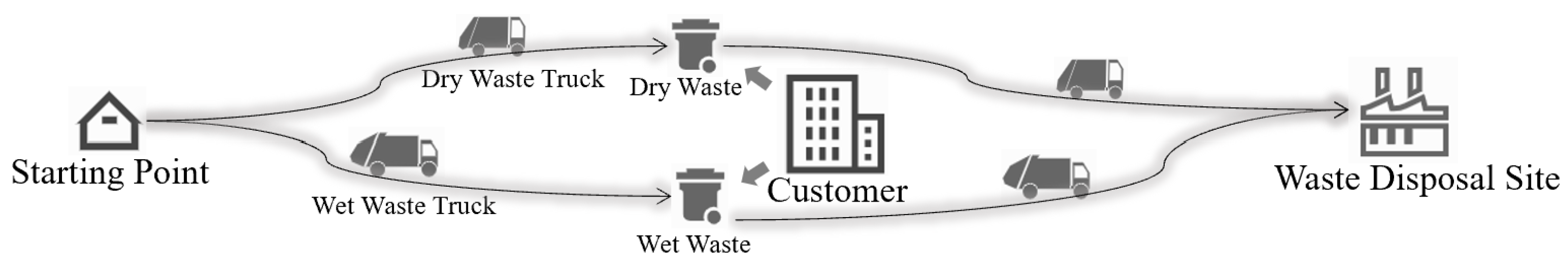
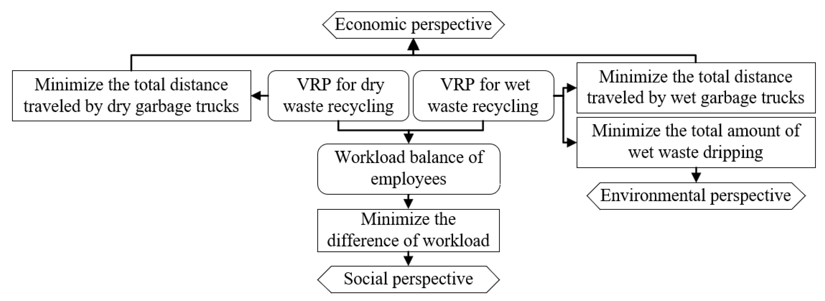
This paper investigates the problem of routing optimization and collection of dry and wet waste, which is considered in an integrated manner from the three pillars of sustainable development, first discussing the two types of products separately from the economic and environmental aspects and integrating the transportation problems of the two types of products from the social aspect. From an economic point of view, the objective of minimizing the collection routes of dry and wet waste is considered. In addition, from an environmental point of view, the objective of minimizing the leakage of wet waste is considered. Finally, from the social perspective, the workload balance between employees handling different types of waste is considered. The transportation process is shown in Figure 1, and its model description diagram is shown in Figure 2.

In this scenario, the waste trucks depart from the starting point and arrive at the waste disposal site after passing a number of customers in a day, and each customer needs to be served once by a dry and a wet waste truck. The journey of a truck from the starting point to the waste disposal site is taken as a route, and there is no limit to the number of routes traveled by each truck per day. Through the optimal combination of different routes, the effective allocation of vehicle resources is achieved while reducing the amount of leakage. In addition, it is necessary to consider the workload balance between employees with different work, and this paper analyzes the length of the routes to derive the optimization of the employee’s efficiency.

3.2. Assumptions and Indices

This paper abstracts and simplifies certain mathematical problems, among which the specific assumptions are as follows:

Assumption 1.

The locations of the starting point, customer, and waste disposal site are known, and there is only one starting point and one waste disposal site.

Assumption 2.

The dry and wet wastes are, respectively, transported by a fleet of fixed-size waste trucks, and the two types of vehicles are sufficient and there is no shortage problem.

Assumption 3.

The employees collecting dry and wet wastes are independent, and there is a fixed upper limit for the employees’ daily working hours.

Assumption 4.

As long as the workload does not exceed the upper limit, the trucks can return to the starting point and start again after reaching the waste disposal site.

Assumption 5.

An employee works with only one truck on a single day, and the employee’s workload can be measured by the route length of the truck.

Assumption 6.

Wet waste may leak, and the degree of leakage is related to the leakage probability, amount of waste carried, and travel distance.

The sets, parameters, and decision variables are defined as in

Table 2. Sets, parameters, and decision variables in model.

Indices and Sets
N	the set of all points, including starting, customer, and waste disposal site, where 0 represents the starting point and 1 represents the waste disposal site
$N^{\prime }$	the set of all customers
i,j	the index of starting points, customers, and waste disposal sites, $i,j\in N$
k	the index of recovered vehicles
$K^{g\left(s\right)}$	the set of all vehicles
Parameters
$d_{ij}$	the distance from vertex i to j, $i,j\in N$
$c_i^{g\left(s\right)}$	the waste production of vertex i, $i\in N^{\prime }$
$L^{g\left(s\right)}$	the maximum load of a waste truck
$v^{g\left(s\right)}$	the average speed of a waste truck
D	the upper limit of the single-day driving distance of the waste truck
T	the maximum number of hours an employee can work in a single day
$\beta$	the probability of leakage during the travel
Decision variables
$x_{ijk}^{g\left(s\right)}$	the 0–1 variable that measures whether the routing from vertex i to vertex j is covered in k. If the routing is covered, the corresponding value is 1; otherwise 0, $i,j\in N$
$y_{ik}^{g\left(s\right)}$	the 0–1 variable, when vertex i is served by vehicle k takes the value of 1; otherwise 0, $i\in N^{\prime }$
$y_{ijk}^{g\left(s\right)}$	the 0–1 variable, takes the value 1 when vertex i is served by waste truck k before j, and i, j is on the same route; when i, j are at the same point and served by a waste truck, the variable indicates that i is served by k and takes the value of 1; otherwise 0, $i,j\in N^{\prime }$
$z_{ijk}^{g\left(s\right)}$	the 0–1 variable, when vertices i, j are served by waste truck k on the same route, the value is 1; when i, j are at the same point, the variable indicates that i is served by k and takes the value 1; otherwise 0, $i,j\in N^{\prime }$

.

Based on the above problem description and assumptions, we need to construct the intermediate variables measuring the length of each route and workload of each employee, so as to facilitate the subsequent analysis and construction of the objective function.

From the starting point, the total distance contains the distances of both wet and dry waste trucks. The expressions for each vehicle’s travel distance is as follows:

$$\begin{array}{c}{D}_k^{g\left(s\right)}={\displaystyle \sum _{i\in N}}{\displaystyle \sum _{j\in N}}{x}_{ijk}^{g\left(s\right)}{d}_{ij},\hspace{1em}k\in K^{g\left(s\right)},\hfill \end{array}$$

(1)

where $d_{ij}$ is the distance between i and j, $D_k^{g\left(s\right)}$ is the distance traveled by vehicle k.

According to Assumption 5, an employee follows only one truck throughout the day, and the workload of the employee can be measured by the running time of the truck. The expression is as follows:

$$\begin{array}{c}{t}_k=D_k^{g\left(s\right)}/v^{g\left(s\right)},\hspace{1em}k\in K^{g\left(s\right)},\hfill \end{array}$$

(2)

where $D_k^{g\left(s\right)}$ is the total length of the route traveled by vehicle k.

According to Assumption 6, the current load weight of the vehicle as it passes through each vertex needs to be considered for calculating the degree of leakage. The amount of wet waste when the vehicle passes through point i is

$$\begin{array}{c}{l}_i^s={\displaystyle \sum _{j\in N^{\prime }}}{\displaystyle \sum _{k\in K^s}}{y}_{ijk}^s{c}_j^s,\hspace{1em}i\in N^{\prime },\hfill \end{array}$$

(3)

where $c_j^s$ denotes the amount of wet waste at point j. Adding up the amount of wet waste at all eligible points is the current load of the wet waste truck when it reaches point i.

3.3. Mathematical Model

Based on the above problem description, this paper considers the separate collection and transportation process of dry and wet wastes; proposes the three objectives of minimizing the total distance, balancing the workload, and minimizing the total amount of leakage from the economic, social, and environmental perspectives; and proposes the constraints in terms of vehicle transportation route selection, the employee working time, and vehicle load. The mathematical model is expressed as follows:

$$min\left(\sum _{k\in K^g}{D}_k^g+\sum _{k\in K^s}{D}_k^s\right)\hspace{1em}\hspace{1em}$$

(4)

$$min\left(\underset{x,y\in \{D_k^g,D_k^s|k\in K^g,K^s\}}{max}|x-y|\right)$$

(5)

$$min\sum _{i\in N^{\prime }}\sum _{j\in N}\sum _{k\in K^s}\beta x_{ijk}^s{l}_i^s{d}_{ij}\hspace{1em}\hspace{1em}$$

(6)

Subject to

$$\sum _{k\in K^{g\left(s\right)}}{y}_{ik}^{g\left(s\right)}=1,\hspace{1em}i\in N^{\prime }\hspace{1em}\hspace{1em}\hspace{1em}\hspace{1em}\hspace{1em}\hspace{1em}\hspace{1em}$$

(7)

$$\sum _{i\in N^{\prime }}{x}_{0ik}^{g\left(s\right)}=\sum _{i\in N^{\prime }}{x}_{i1k}^{g\left(s\right)},\hspace{1em}k\in K^{g\left(s\right)}\hspace{1em}\hspace{1em}\hspace{1em}\hspace{1em}$$

(8)

$$\sum _{i\in N^{\prime }}\sum _{j\in N^{\prime }}{x}_{ijk}^{g\left(s\right)}=\sum _{i\in N^{\prime }}{y}_{ik}^{g\left(s\right)}-\sum _{i\in N^{\prime }}{x}_{0ik}^{g\left(s\right)},\hspace{1em}k\in K^{g\left(s\right)}\hspace{1em}$$

(9)

$$\sum _{i\in N}\sum _{k\in K^{g\left(s\right)}}{x}_{ijk}^{g\left(s\right)}=\sum _{i\in N}\sum _{k\in K^{g\left(s\right)}}{x}_{jik}^{g\left(s\right)}=1,\hspace{1em}j\in N^{\prime }\hspace{1em}$$

(10)

$$\sum _{i\in N^{\prime }}{z}_{ijk}^{g\left(s\right)}{c}_i^{g\left(s\right)}\le L^{g\left(s\right)},\hspace{1em}k\in K^{g\left(s\right)},j\in N^{\prime }\hspace{1em}\hspace{1em}\hspace{1em}$$

(11)

$$D_k^{g\left(s\right)}/v^{g\left(s\right)}\le T,\hspace{1em}k\in K^{g\left(s\right)}\hspace{1em}\hspace{1em}\hspace{1em}\hspace{1em}\hspace{1em}\hspace{1em}$$

(12)

$$\sum _{j\in N}{x}_{ijk}^{g\left(s\right)}=y_{ik}^{g\left(s\right)},\hspace{1em}i\in N^{\prime },k\in K^{g\left(s\right)}\hspace{1em}\hspace{1em}\hspace{1em}\hspace{1em}$$

(13)

$$\sum _{i\in N}{x}_{ijk}^{g\left(s\right)}=y_{jk}^{g\left(s\right)},\hspace{1em}j\in N^{\prime },k\in K^{g\left(s\right)}\hspace{1em}\hspace{1em}\hspace{1em}\hspace{1em}$$

(14)

$$x_{ijk}^{g\left(s\right)}\le y_{ijk}^{g\left(s\right)}\le z_{ijk}^{g\left(s\right)},\hspace{1em}i,j\in N,k\in K^{g\left(s\right)}\hspace{1em}\hspace{1em}\hspace{1em}$$

(15)

$$x_{ijk}^{g\left(s\right)},y_{ik}^{g\left(s\right)},y_{ijk}^{g\left(s\right)},z_{ijk}^{g\left(s\right)}\in \{0,1\},\hspace{1em}\forall i,j\in N,\forall k\in K^{g\left(s\right)}$$

(16)

Equation (4) is to minimize the total travel distance; Equation (5) is to balance the workload of employees, minimizing the maximum distance difference between the vehicles driven by the employees responsible for the two types of waste in a day; and Equation (6) is to minimize the total leakage, which is related to the amount of wet waste carried and length of the route.

Equations (7)–(10) are constraints on the vehicle route, Equation (11) is the capacity constraint, and Equation (12) limits the maximal working hour an employee can work in a single day. Equations (13)–(16) state the interconnections and constraints between decision variables.

The model constructed in this paper is a multi-objective 0–1 integer nonlinear programming, and the commonly used software, such as CPLEX, cannot directly solve it. Additionally, in practical waste collection problems, the number of customer points are relatively huge in size, which will increase the dimensionality and constraints of the decision variables and the computational complexity, and the traditional algorithms, such as branch-and-bound and cut-plane, are not suitable for solving such large-scale problems. Therefore, a multi-objective evolutionary algorithm needs to be designed for solving the problem.

4. Solution Method

4.1. Basic Principle of NSGA-III Algorithm

NSGA-III algorithm [42] is a multi-objective evolutionary algorithm that makes improvements on the basis of NSGA-II, which is inspired by scholars based on the law of biological selection, elimination, and survival of the fittest in nature. The algorithm treats all decision variables as a chromosome or an individual and uses the objective function as the evaluation criterion for the fitness. In each iteration, chromosomes are selected, crossed, and mutated, so that the fitness value is gradually enhanced and the chromosome can be easier to survive to the next iteration.

The main idea of NSGA-III is to introduce a reference point mechanism based on NSGA-II [43] and to retain individuals close to the reference point. The main difference between the two algorithms is the change in the selection mechanism and criteria for judging the merit of Pareto’s rank. NSGA-III adapts the crowding degree ranking and introduces widely distributed reference points to ensure the diversity of the retained populations in each iteration.

Unlike the MOEA/D algorithm [44], NSGA-III does not require any additional parameters setting during execution. Moreover, its excellent ability to solve many different types of multi-objective problems and handle a small number of user-supplied structured or randomly assigned reference points has been widely tested. Therefore, it is suitable for multi-objective preference-based optimization and decision making, and this paper solves the proposed problem by improving the NSGA-III algorithm.

4.2. Improved NSGA-III Algorithm

The improved NSGA-III makes improvements in three aspects: firstly, the generated initial solution is optimized using the probabilistic insertion method; secondly, the Metropolis criterion of the simulated annealing algorithm is added in the crossover process to accept inferior solutions after a crossover with certain probability; and thirdly, the adaptive mutation operator is added in the mutation process to ensure population diversity. This paper focuses on the specific improvements and simplifies the overall steps of the algorithm; please refer to Deb [42] and Ishibuchi [45] for detailed steps.

4.2.1. Initial Solution Generation

The initial solution of VRPs is usually generated by random generation method [46], nearest insertion method [47], greedy algorithm [48], sweep algorithm [49], probabilistic insertion method, etc. And we improved the nearest insertion method by combining it with the nearest neighbor and saving methods for solving the VRP.

The principal of the proposed improved probabilistic insertion method is to determine the order of all the customer points based on the length of route, weight of waste, and vehicle’s capacity. Take the wet waste as example; the specific process of the method for generating a chromosome is described as Algorithm 1.

Algorithm 1 Processes of the improved probabilistic insertion method

1: Determine a route with only two points, i.e., the starting point and the waste disposal site. 2: Find out the set of customer points meet the load constraint. 3: Select the customer point with a certain probability which is inversely proportional to the product of route length and wet waste weight, insert it into the position before the endpoint of the current route, and take it as the starting point for selecting the next customer point to be inserted. 4: Repeat steps 2 and 3 until the vehicle is fully loaded or its remaining capacity is less than the weight of waste at any customer point. 5: Start a new route when the vehicle’s capacity is exceeded and repeat steps 1 to 4 until all the customer points are inserted to the route.

4.2.2. The Steps of the Improved NSGA-III

The steps of the improved NSGA-III are as follows:

Step 1: Coding. Because the customer points are discretely distributed, this paper adopts the natural number coding method. Set the departure point as 1, the waste disposal site as M, and all the customers as 2, 3, …, $M-1$, respectively.

Step 2: Initialization. Use the probabilistic insertion method to generate the initial solution of wet waste with the smallest possible total amount of leakage and the initial solution of dry waste with the smallest possible total distance. Set the basic parameters, such as the size of the problem and population, the crossover and mutation probability, and the number of iterations.

Step 3: Adaptation decoding. Calculate the fitness value of each chromosome and record as a triple consisting of three objective function values. And then calculate the average fitness value of all the chromosomes for evaluating the overall quality of the solution set.

Step 4: Non-dominance ranking. Find the individuals that are not dominated by others in the population and record them as Pareto rank 1; remove the individuals with Pareto rank 1, find the individuals that are not dominated by others in the remaining set and mark them as Pareto rank 2; repeat the above operations until all the individuals are marked with Pareto rank.

Step 5: Crossover. Utilize the Metropolis criterion to compare the superiority and inferiority of the incidental and offspring chromosomes. When the new solution obtained by crossover is inferior to the old one, accept the inferior solutions with a certain probability:

$$P_m^g=P_m·{\alpha }^g,$$

(17)

where g is the current number of iterations, $P_m^g$ is the mutation probability at the gth iteration, $P_m$ is the initial mutation probability, and $\alpha$ is 1.005 ($\alpha$ is a random number from 1.001 to 1.4). As the iteration progresses, the mutation probability becomes progressively larger.

The operation is stopped when all the alternative chromosomes have completed the crossover operation and a new population is obtained. At the same time, the best individuals that have emerged so far in the population during the evolutionary process are replicated to the next generation by an elite retention strategy.

Step 6: Mutation. Record the elements in some segments of selected individuals, and add an adaptive mutation operator to increase the mutation probability with iteration at this point. The same elite retention strategy is used throughout the mutation process. The mutation probability is calculated by

$$y=e^{d/\left({\lambda }^g\right)}$$

(18)

where d is the difference between the normalized summed average of the three objective functions of the superior solution before each iteration and that of the inferior solution after, $\lambda$ is 0.99 ($\lambda$ is a random number from 0 to 1), and g is the current number of iterations. Because d takes a negative value, the acceptance probability of the inferior solution will gradually become smaller as the iteration proceeds.

Step 7: Select new population. Merge the parent and offspring populations that have undergone crossover and mutation, and retain the individuals with higher fitness values to form a new population for the next iteration.

Step 8: Terminate iteration. The algorithm stops when the fitness values in the Pareto solution set obtained at each iteration do not change within L generations.

Step 9: Output Pareto solution set. Select the individuals with Pareto rank 1 after each generation of completed iterations is merged, and form the final Pareto solution set.

The framework of the improved NSGA-III is shown in Figure 3.

5. Performance Verification

In Section 4, the improved NSGA-III uses the improved probabilistic insertion method to generate the initial waste collection route and adds the Metropolis criterion of the simulated annealing algorithm and the adaptive mutation operator to ensure population diversity. In this section, we validate the initialization process and compare the proposed algorithm with the classic NSGA-II and NSGA-III to verify its effectiveness.

5.1. Experimental Design

In this paper, the Solomon standard datasets are used for testing (Source of Solomon dataset: http://w.cba.neu.edu/msolomon/problems.htm (accessed on 20 June 2022)). These datasets are randomly generated based on certain distribution characteristics, containing information such as the X- and Y-coordinate axes of each point, customer number and their demands, vehicle number, and their load capacity. The Solomon datasets can be divided into three categories according to the distribution types: R-type with a random distribution of customer points, C-type with an aggregated distribution of customer points, and RC-type with both of them.

In this paper, we have selected six datasets containing 100 customer points for verification, and the parameters of them are shown in

Table 3. Parameters of standard dataset.

Categories	Number of Customers	Vehicle Capacity	Type of Data	Number of Files
C1	100	200	Cluster distribution	9
C2	100	700	Cluster distribution	8
R1	100	200	Random distribution	12
R2	100	1000	Random distribution	11
RC1	100	200	Mixed distribution	8
RC2	100	1000	Mixed distribution	8

. The leakage coefficient $\beta$ is assumed as 0.0001, the travel speed is 50 km/h, and the maximum working hour is 8.

5.2. Initial Solution Comparison Analysis

First, the proposed probabilistic insertion method considering the total distance or leakage is compared with the random generation method, greedy algorithm, and nearest insertion method. The locations of the points and demands of dry waste are extracted from dataset RC101, and the demands of wet waste are from dataset C102. All the demands are roughly between 10 and 50 tons. The distance between each two points are calculated as the Euclidean distance. The algorithm parameters used are shown in

Table 4. Algorithm parameters.

Parameters	Value	Parameters	Value
Population size	100	Maximum number of iterations	500
Crossover probability	0.8	Initial mutation probability	0.15

.

The average fitness values in the solution set with Pareto rank 1 after 10 runs of each method are shown in

Table 5. Comparative results generated by different methods.

Initial Methods	Eco	Soc	Env	Eco*	Soc*	Env*	Number of Iterations
Random generation method	4231	220	3.60	2789	120	2.21	180
Greedy algorithm	2534	205	3.03	2320	135	2.08	145
The nearest insertion method	3020	180	2.83	2762	124	1.90	164
Probabilistic insertion method	2879	158	2.78	2414	105	1.80	120

Note: Eoc, Soc, and Env represent the initial solution of total distance, the route-length difference, and the total amount of leakage separately solved using the initialization method. Eoc*, Soc*, and Env* represent the corresponding optimal solution obtained after algorithm iteration, and values in bold represent the minimum value of Eoc*, Soc*, and Env* respectively.

. It can be seen that in the initial population, the probabilistic insertion method surpasses the other methods in the total amount of leakage and route-length difference with the minimum number of iterations, indicating that the probabilistic insertion method performs relatively better in convergence.

5.3. Performance Analysis of the Improved NSAG-III

The performance of the improved NSGA-III is verified by comparing with the classic NSGA-II and NSGA-III in terms of four evaluation metrics: the number of convergence iterations, ideal value of individual objectives, fitness value, and Pareto solution.

(1)

Number of convergence iterations

The algorithm is set to reach convergence when the ideal values of the three objective function values of the population do not appear better after 10 iterations, and the number of iterations shows the convergence speed of the algorithm.

Table 6. Comparison of the number of iterations of different algorithms.

Number	NSGA-II	NSGA-III	Improved NSGA-III
1	140	124	104
2	152	199	125
3	109	129	93
4	162	117	89
5	160	126	135
6	100	191	109
7	128	136	111
8	131	120	149
9	180	73	139
10	189	133	144
Average	145	134	120
Coefficient of variation	0.20	0.27	0.18

illustrates the performance of these algorithms in convergence. We can see that both the average number of the convergence iterations and the coefficient of the variation of the improved NSGA-III are less than those of the classic NSGA-II and NSGA-III, showing that the improved NSGA-III exhibits higher stability in terms of convergence speed.

(2)

The ideal values of objective function values

The ideal value is the optimal value of each objective function in a population. After obtaining the Pareto solution set of each iteration, the minimum value of each objective function is retained so as to observe the change in the ideal value with the number of iterations. The maximum number of iterations is set as 300 to ensure that the convergence is finally reached. As shown in Figure 4, the improved NSGA-III has better ideal values than the other two algorithms in terms of the total distance, route-length difference, and total amount of leakage.

(3)

Fitness value

Different from the ideal values of each objective function in the Pareto solution set obtained by each iteration which can only show the optimal performance of the algorithm in each objective dimension, the average fitness value of the Pareto solution set can reflect the overall quality of the entire solution set.

Table 7. Comparison of fitness value of different algorithms.

Objective Function Value	Eco*	Soc*	Env*
Average of NSGA-II	2854	129	2.44
Average of NSGA-III	2765	130	2.22
Average of improved NSGA-III	2616	118	2.20
Ideal value of NSGA-II	2629	120	2.29
Ideal value of NSGA-III	2581	111	2.05
Ideal value of improved NSGA-III	2450	106	1.93

Note: Eoc*, Soc*, and Env* represent the optimal solution of the total distance, the route-length difference, and the total amount of leakage.

shows that the average value of the improved NSGA-III is optimized by 8.3 and 5.3% in terms of the total distance, 9.1 and 9.2% in terms of the route-length difference, and 9.8 and 0.9% in terms of the total amount of leakage than the classic NSGA-II and NSGA-III, indicating that the improved NSGA-III performs the best in terms of the overall quality of the Pareto solution set.

(4)

Pareto solution

One quantitative measure of algorithm performance is the number of Pareto solutions, and a higher value of this number indicates that it is more appropriate [50,51]. Figure 5 presents the distribution of the Pareto solution sets obtained by the three algorithms in one operation, where Figure 5a is the integrated plot of Pareto solution sets and Figure 5b–d are the projections of Pareto solution sets on different two-dimensional planes, showing more clearly the distribution of the solution sets on different axes. The numbers of Pareto solutions with rank 1 derived from three algorithms are 170, 142, and 368, respectively.

As can be seen in Figure 5, the solution set obtained by the improved NSGA-III is in the lower middle position and performs better than the other two algorithms with a smaller total amount of leakage, total distance, and route-length difference.

In order to obtain more reliable results of the algorithms’ performance analysis, we generate more examples with the Solomon datasets and compare the three algorithms according to the above process, and the results obtained are basically the same. Based on all these results, the following conclusions can be drawn:

(1)

The improved NSGA-III converges faster than the other two algorithms. The initial population of the improved NSGA-III is optimized for both the total distance and amount of leakage, while the classic NSGA-II and NSGA-III use randomly generated initial solutions, thus reaching a solution close to the optimal value requires fewer iterations.

(2)

The improved NSGA-III has the highest quality of the solution set. In terms of ideal values, the comparison algorithms may fall into local optimal solutions. The improved NSGA-III incorporates the Metropolis acceptance criterion of the simulated annealing algorithm and the adaptive mutation probability, ensuring a higher probability of searching for solutions with a better performance in ideal values while the population diversity is improved.

6. Case Study of Shanghai City

In this section, the improved NSGA-III is applied to solve and analyze the real case of the Xujiahui subdistrict in the Xuhui District, Shanghai. The data are preprocessed first, and the final solution is selected from the resulting Pareto solution set. Then, the route before and after waste classification are compared, and the parameters sensitivity analyses of the maximum working hour, vehicle load capacity, and weight of waste are conducted. Finally, the management insights are given to ensure that the company has a high level of competition.

6.1. Background Description

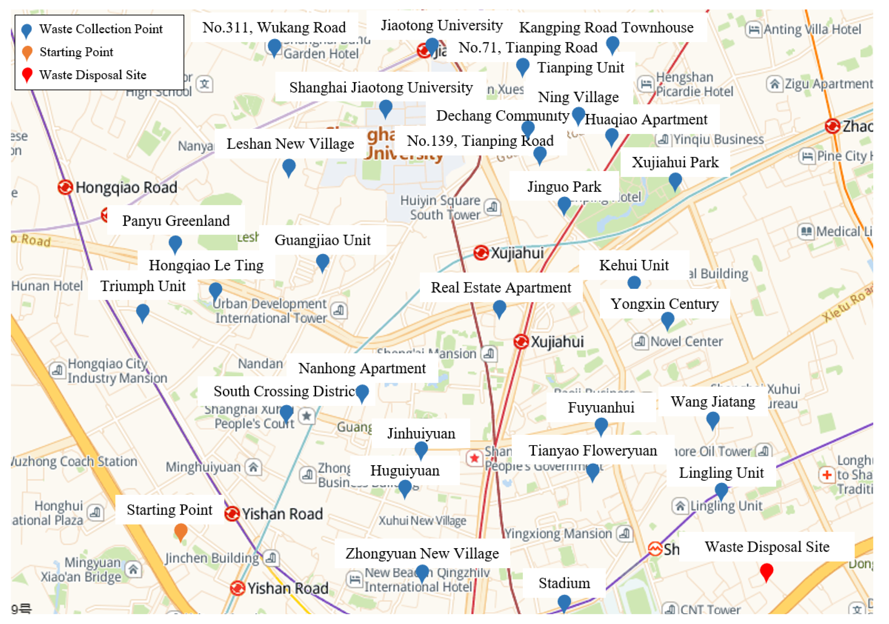
Xujiahui Street is a subdistrict located in the central and western part of the Xuhui District. There are currently 248 customer points in this area, and some of them are close to each other. Hence, the gravity method is utilized to merge the adjacent customer points into a collection point, and a set of 30 barycenters with their coordinates are obtained. The geographic locations of the collection points, starting point, and waste disposal site are shown in Figure 6. Three sanitation companies are responsible for collection in this area, and there are a total of 128 dry waste trucks with a load capacity of 5 tons and 50 wet waste trucks with a capacity of 3 tons.

Assume that the maximum working hour of employees is 8 h, and the average speed of the trucks is 50 km per hour. Then, we apply the proposed model and algorithm to find the Pareto set and select the optimal solution, comparing the differences between the results before and after waste classification.

6.2. Optimal Solution Selection

Before the specific routing optimization, the distances between each two points are calculated according to Equation (19),

$$d=R·arccos[cos(Y1)·cos(Y2)·cos(X1-X2)+sin(Y1)·sin(Y2\left)\right].$$

(19)

where $R=6371$ km is the radius of the earth, and $(X1,Y1),(X2,Y2)$ are the latitude and longitude coordinates of points 1 and 2.

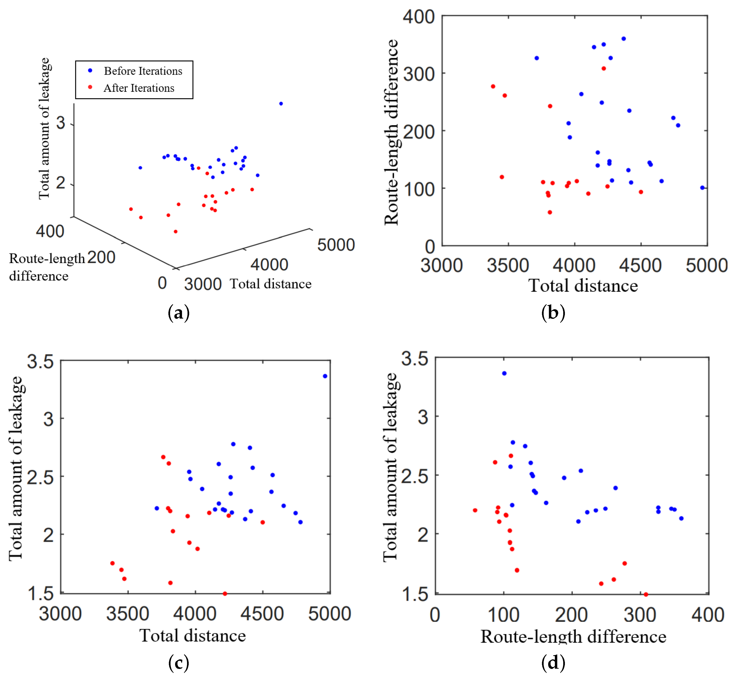
In the process of solving with the improved NSGA-III, the initial and final Pareto sets can be obtained, and the spatial distribution and two-dimensional projections are shown in Figure 7, where the blue and red dots represent the Pareto sets before and after the iterations, respectively.

The comparison shows that in terms of the total amount of leakage, the quality of the final solutions are mostly significantly better than that of the initial solutions. In terms of the route-length difference, the overall quality of the final Pareto set has improved significantly, with smaller values than at the initial one. A large improvement is also achieved in terms of the total distance, with only two of the optimal solutions taking closer values to the initial solution set. The above results further demonstrate that the iteration process can significantly improve the overall quality of the Pareto solution set.

After combining all the Pareto solutions in each generation, the final 127 Pareto optimal solutions are obtained, and the final collection routing scheme can be decided according to the decision maker’s preference.

As an economically prosperous area, the government of the Xuhui District is more concerned about the impact of waste collection on the environment than the economic cost and personnel balance of waste collection and hopes that the total amount of leakage in the transportation process will be as small as possible. Therefore, the decision maker can first sort the Pareto solution set and divide it into different intervals according to the total amount of leakage. Subsequently, assume that the decision maker attaches equal importance to the total distance and route-length difference and normalize the values of these two objective functions of each solution in the same interval. Then, add the sum of the three objective function values, as shown in

Table 8. Pareto solution set objective function value.

No.	Env*	Eco*	Soc*	Normalized Sum
1	1.49	4719	308	2
2	1.58	4314	242	1.70
3	1.61	3972	260	1.68
4	1.69	3450	109	1.08
5	1.75	3884	276	1.72
6	1.86	4463	317	1.86
7	1.87	4515	112	1.23
8	1.93	4455	109	1.21
9	1.94	5149	113	1.35
10	1.96	4567	117	1.25
...	...	...	...	...
123	3.05	4547	75	1.46
124	3.10	4858	98	1.71
125	3.14	4462	120	1.81
126	3.36	5462	100	1.83
127	3.46	5370	64	1.52

Note: Eoc*, Soc*, and Env* represent the optimal solution of the total distance, the route-length difference, and the total amount of leakage. The rows in boldness represent the optimal solution for different total amount of leakage ranges.

.

As we can see, among the 127 scenarios, the total amount of leakage ranges from 1.49 to 3.46 tons. According to the numerical results in Table 5 and Table 6, if the government’s allowed range for the total amount of leakage is 1.4–1.8 tons, then the optimal should be selected from the first interval, and Scheme 4 with the minimal normalized sum is the optimal option, of which the total distance and route-length difference are both significantly smaller than other schemes. If the allowable range is 1.8–2.0 tons, then Scheme 8 is the optimal solution, and if the allowable range is 3.0–3.5 tons, option 123 is the optimal solution.

Note that the solution in this paper only provides a reference for companies to select the optimal solution. If the company’s most important goal is not the total amount of leakage, or if the total distance and the route-length difference are not equally important, the method of selecting the optimal solution can be adjusted.

6.3. Comparison of Routing Optimization Results

This section compares the routing results of the changes for sanitation companies in terms of routes, personnel, and vehicles, before and after waste classification.

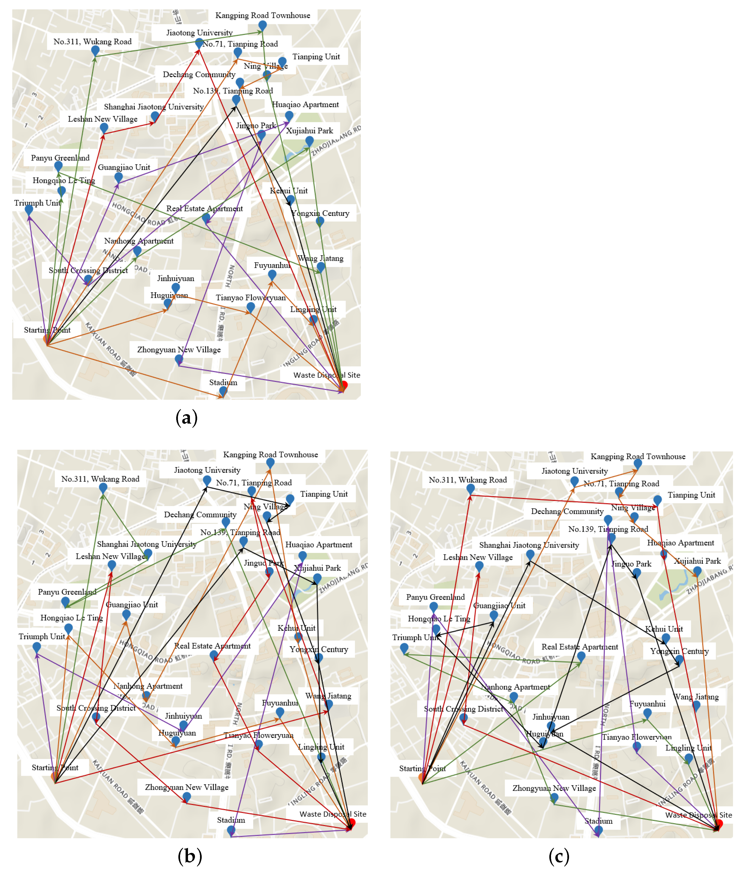
Figure 8 presents the routes before waste classification and the separate dry and wet waste collection routes after classification, where the lines in the same color represent the routes of the same vehicle. Before the waste classification, the weight of the waste at each point is the sum of the dry and wet wastes weight, and the load capacity of each vehicle is 5 tons. The solution that meets the load capacity and maximum working hour of employees with the smallest total distance is found in the routing arrangement, and the solution after the classification is Scheme 4 in Table 8. To make the map readable, all routes from the waste disposal site back to the starting point are omitted here.

By comparison, it can be found that the route before the classification is a collection of some points close to each other because only the total distance and vehicle capacity are considered. However, because of the mixed loading of the dry and wet waste, the weight of the waste at each collection point is heavier; thus, the number of collection points on a single route is less than the number after the waste classification, and some points farther apart than others with less weight of waste appear in some routes. In contrast, the routes after the classification are results of the trade-off between multiple objectives, and thus the spatial distribution of points on the same route are more dispersed.

The comparative results of the optimal solutions before and after the classification are shown in

Table 9. Comparison of waste collection and transportation results.

	The Value of Objective Function			Number of Employees	Number of Vehicles	Route-Length Difference
	Eco*	Soc*	Env*			Dry Waste	Wet Waste
Before classification	1803	410		5	5
After classification	3450	109	1.69	10	10	108.8	106.2

Note: Eoc*, Soc*, and Env* represent the optimal solution of the total distance, the route-length difference, and the total amount of leakage.

, from which we can see that before the classification, only economic factors are considered, and the total distance is 1803, nearly half less than that after the classification. By substituting 1803 into the objective function of workload balance, a route-length difference of 410 can be derived, which is far more than the result after the classification. Because of a more detailed division of labor among employees, the workload balance after classification was optimized by 276%.

In addition, with regard to manpower and material resources, only five employees and five trucks are needed for waste collection before the classification. After the classification, however, collecting dry and wet wastes requires 10 employees, 5 dry waste trucks, and 5 wet waste trucks, meaning that the company needs to purchase 5 wet waste trucks and recruit 5 new employees. Given that the cost of wet waste trucks is roughly 70,000 CNY each and the monthly salary of employees is about 5000 CNY, then the company’s operating cost doubles.

In order to analyze the influence of the route-length difference and total amount of leakage on the route selection, this section also considers three models with different objective functions, the results of which are shown in

Table 10. Comparison of model results considering different objective functions.

Models	Objectives	Eco*	Soc*	Evn*
Model 1	Consider three objectives at the same time	4042	131	1.9
Model 2	Total distance + total amount of leakage	3526	173	1.4
Model 3	Total distance + route-length difference	3733	121	2.1

Note: Eoc*, Soc*, and Env* represent the optimal solution of the total distance, the route-length difference, and the total amount of leakage.

.

As we can see, without considering social factors, Model 2 performs poorly in terms of the workload balance, which will cause a great injustice in real life and interfere with company operations. And if the environmental impact is not considered, Model 3 performs poorly in terms of the total amount of leakage, which can have a large impact on the environment and thus affect the company’s operations. For sanitation companies, the priority is not economic factors but social and environment factors, so the biggest advantage of Model 1 is that it starts from the actual situation and balances the operations from multiple aspects.

6.4. Sensitivity Analyses

Based on actual data, the sensitivity analyses of three parameters, maximum employee working time, vehicle load, and waste weight, are conducted in this section.

By plus or minus 10 and 20% of the initial setting of the maximum working hour of 8 h, we obtain five values between 6.4 and 9.6 h, and show its effect on the optimization routing scheme in Figure 9. It can be seen that with the growth of the maximum working hour of employees, the route-length difference increases, yet the total distance and wet waste leakage change irregularly. The reason is that when arranging the driving routes, it is always desired that employees work as long as possible, but some employees will not be able to approach the maximum working hour limited to the vehicle load capacity and number of waste collection points. According to the results, the sanitation company should specify a reasonable maximum working hour for employees, ensure a relatively reasonable workload distribution, and give corresponding remuneration to the employees, so as to better motivate them.

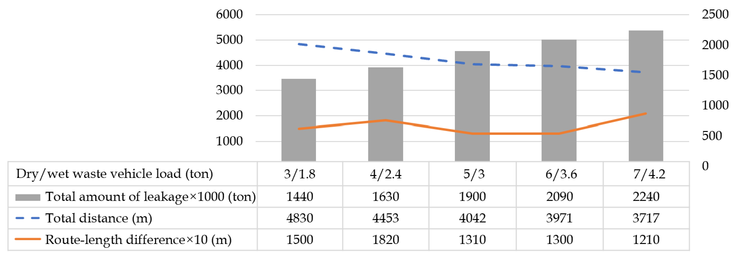
Figure 10 shows the effect of the maximum vehicle load capacity on the final optimization scheme, which is set to 5 and 3 tons initially. Here, the ratio of dry and wet waste load capacity is kept constant, and 3/1.8, 4/2.4, 5/3, 6/3.6, and 7/4.2 tons are selected for the sensitivity analyses. It can be seen that the total distance and wet waste leakage increases with the increase in vehicle load capacity, whereas the route-length difference is not significantly correlated. It may be because with the vehicle load capacity increases, one vehicle can travel to more waste collection points and accordingly reduce the total number of trucks going to and departing from the starting point and waste disposal site. In addition, the increase in leakage is caused by the increasing load during a single route and a smaller change in the distance traveled between points. Therefore, the sanitation companies can consider using some heavy-duty vehicles for transportation. At the same time, in order to protect the environment, they shall purchase wet waste trucks with stronger sealing properties.

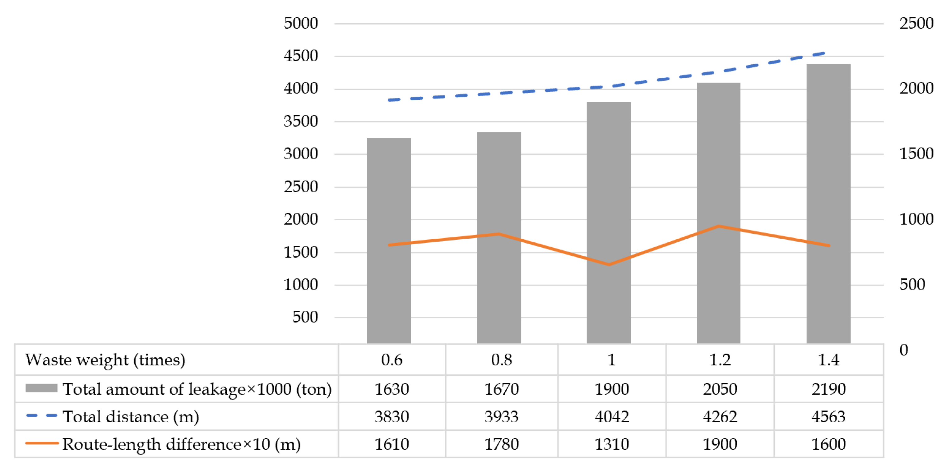
The influence of the waste weight on the routing scheme is shown in Figure 11. For comparison, 0.6, 0.8, 1, 1.2, and 1.4 times of the initial weight of 1 are taken. As we can see, the total distance and total amount of leakage both increase with the waste weight, while there is no significant relationship between the difference in the route-length and the change in the waste weight. As the waste weight increases, the average load of the vehicle during transportation will rise, and accordingly, the vehicle will travel to less waste collection points on a single route due to the load limitation, resulting in a greater total distance. Both of these factors will increase the total amount of wet waste leakage. Henceforth, the sanitation companies should consider using vehicles with a larger load capacity and ensure that the total driving distance is as small as possible by rationally arranging vehicle routes.

We use the objective values as the dependent variable and perform a one-way ANOVA for each of the above three scenarios. The results show that the significance level p-values are 1, 0.999, and 0.992, respectively, all greater than 0.05, indicating that there is no significant difference between the results, which means the maximum working time, the waste vehicle load, and the waste weight will not affect the results.

6.5. Discussion and Management Insights

The results of the numerical analysis above show that the company’s actual transport routes change significantly after the waste classification, more waste collection points are served on a single route, and the distribution on the same route is more dispersed. The total distance nearly doubled after the classification, and most of the subsidies received by the company were used to purchase new vehicles. If there were not enough funds to recruit new employees, this would result in a significant increase in the number of hours worked by the employees and reduce their job satisfaction. Therefore, the company needs to take into account the change in the employee workload and solve the problem of employee satisfaction by increasing the salary performance or recruiting new employees.

From the comparison before and after the waste classification, we have found that the routes after the classification are more chaotic than before, because it is necessary to obtain a more suitable route scheme while keeping the total distance as small as possible and taking into account the route-length difference in employees and total amount of leakage. The company is balancing the workload of the wet and dry waste collection employees, because it is difficult to balance the route-length difference on a single day (from Table 10, we can see that the average value of the employee-distance difference is 131 km, which is about 2.6 h of working-hour difference), the company can try to introduce a shift scheduling system, so that the employees can travel different routes every day and ensure a workload balance over a longer period.

The leakage coefficient in this paper is set to 0.0001, which is relatively small, but the leakage is still a considerable amount, which will aggravate the pressure of road cleaning along the transportation process in the long run. From a long-term perspective, companies should try to choose wet waste trucks with better enclosures and better treatment for leakage prevention, but perhaps at a higher unit cost, in order to reduce the risk of leakage in daily operations and help the sustainable development of the city.

In addition, although the employees responsible for dry and wet waste may have a closer driving time during transportation, the workload will be different when loading and unloading waste, and there is a significant difference in the feeling of waste handling because the smell of wet waste is heavier, which will make the employees more uncomfortable. Companies shall consider from the perspective of a performance system and rotate the employees of dry and wet wastes in a certain cycle, so as to improve the satisfaction as well as the work skills of the employees.

Apart from better servicing to the society, sanitation companies also need to compete with companies in the same industry, so in addition to considering from the perspective of route optimization, companies can also improve their competitiveness from the perspective of service. First, the company can try to refine the collection and transportation of the waste. Because the wet waste contains a large amount of liquid, it is easy to cause liquid leakage and produce odors when the weather is hot. The company can try to increase the frequency of wet waste collection and transportation at night in some areas on the basis of the comprehensive protection of collection and transportation, and effectively reduce the residence time of wet waste in residential areas. Second, the company can try to develop different cleaning programs according to local conditions and create various cleaning work modes, such as chain cleaning and three-dimensional cleaning, for each region. Third, the company can also make improvements in terms of waste trunks. From the company’s long-term planning, it is necessary to fully consider the damage caused by the increase in the weight of waste to the trunk, as well as the load capacity and sealing performance of the new trunk. In addition, the waste trunk can be modified to grasp the vehicle position, running trajectory, and load capacity in real time and connect with the street grid management platform to achieve data interoperability. Through the real-time sharing of information, the perfect docking between the waste trunk and the waste can is realized.

7. Conclusions

The implementation of a waste classification and collection policy plays a very important role in protecting the environment. In order to further promote the policy, Shanghai took the lead in adopting waste classification and collection. However, in the process of implementing the policy, there will undoubtedly be many problems. Environmental protection, employee mentality, and company interests are all factors that need to be considered. Based on the above background, this paper proposes a multi-objective VRP model of waste collection and transportation and an improved NSGA-III algorithm to solve this problem.

First, in this paper, the actual driving route is obtained with consideration of classified waste collection. Although this scheme will increase the driving cost, it can also ensure the workload balance among employees to a certain extent, thus improving the job satisfaction of employees. In addition, this paper considers the leakage of wet waste; the employee has to recycle the waste with as little leakage of wet waste as possible.

Second, in the process of designing the improved NSGA-III, the probabilistic insertion method is mainly used to generate the initial solution, and the effectiveness of the method is verified by comparing it with the greedy algorithm and the nearest insertion method. Then, the quality of the solution is improved by the probability acceptance operator of the simulated annealing algorithm, and the population diversity is further increased by the adaptive mutation operator.

In addition, in order to verify the solution efficiency of the proposed model and algorithm, numerical experiments are illustrated using Solomon datasets, and it can be seen from the experimental results that the algorithm outperforms the other algorithms in terms of the convergence speed and ideal values. In addition, this paper compares the routes before and after waste classification with the real case of the Xuhui District and performs a sensitivity analysis on the parameters so as to provide references for the actual operations of sanitation companies.

Although this paper provides a set of methods that can be used for reference by sanitation companies for waste collection and obtains some research results with theoretical and practical significance, there are still some limitations in this study. Firstly, all the input parameters considered in this paper are definite values, yet there may be uncertain factors in practice. Secondly, the limiting factors of customers’ time windows are not taken into account in this paper. In addition, we assume that there is only one distribution center, in the practical waste collection problem; however, this may be more complex with multiple starting points and waste disposal sites. In the future work, we will model fuzzy or uncertain programming to deal with the indeterminate factors in the transportation process. In addition, the customers can be divided into different areas and then we will derive a more realistic transportation route scheme.

References

1. Tong, Y.; Liu, J.; Liu, S. China is implementing “Garbage Classification” action. Environ. Pollut. 2020, 259, 113707. [Google Scholar] [CrossRef] [PubMed]
2. Xiao, S.; Dong, H.; Geng, Y.; Francisco, M.; Pan, H.; Wu, F. An overview of the municipal solid waste management modes and innovations in Shanghai, China. Environ. Sci. Pollut. R. 2020, 27, 29943–29953. [Google Scholar] [CrossRef] [PubMed]
3. Laureri, F.; Minciardi, R.; Robba, M. An algorithm for the optimal collection of wet waste. Waste Manag. 2016, 48, 56–63. [Google Scholar] [CrossRef] [PubMed]
4. Wang, L.; Zhao, J.; Zhou, K. How do incentives motivate absorptive capacity development? The mediating role of employee learning and relational contingencies. J. Bus. Res. 2018, 85, 226–237. [Google Scholar] [CrossRef]
5. Lieckens, K.T.; Colen, P.J.; Lambrecht, M.R. Optimization of a stochastic remanufacturing network with an exchange option. Decis. Support. Syst. 2013, 54, 1548–1557. [Google Scholar] [CrossRef]
6. Vahdani, B.; Tavakkoli-Moghaddam, R.; Jolai, F. Reliable design of a logistics network under uncertainty: A fuzzy possibilistic-queuing model. Appl. Math. Model. 2013, 37, 3254–3268. [Google Scholar] [CrossRef]
7. Eskandarpour, M.; Masehian, E.; Soltani, R. A reverse logistics network for recovery systems and a robust metaheuristic solution approach. Int. J. Adv. Manuf. Tech. 2014, 74, 1393–1406. [Google Scholar] [CrossRef]
8. Chaabane, A.; Montecinos, J.; Ouhimmou, M.; Khabou, A. Vehicle routing problem for reverse logistics of End-of-Life Vehicles (ELVs). Waste Manag. 2021, 120, 209–220. [Google Scholar] [CrossRef]
9. Delle, D.D.; Di, T.V.; Duran, G. Optimizing leaf sweeping and collection in the Argentine city of Trenque Lauquen. Waste Manag. Res. 2021, 39, 209–220. [Google Scholar] [CrossRef]
10. Delgado-Antequera, L.; Laguna, M.; Pacheco, J.; Caballero, R. A bi-objective solution approach to a real-world waste collection problem. J. Oper. Res. Soc. 2020, 71, 183–194. [Google Scholar] [CrossRef]
11. Galindres-Guancha, L.F.; Toro-Ocampo, E.; Gallego-Rendon, R. A biobjective capacitated vehicle routing problem using metaheuristic ILS and decomposition. Int. J. Ind. Eng. Comp. 2021, 12, 293–303. [Google Scholar] [CrossRef]
12. Mancini, S.; Gansterer, M.; Hartl, R.F. The collaborative consistent vehicle routing problem with workload balance. Eur. J. Oper. Res. 2021, 293, 955–965. [Google Scholar] [CrossRef]
13. Raa, B.; Aouam, T. Multi-vehicle stochastic cyclic inventory routing with guaranteed replenishment. Int. J. Prod. Econ. 2021, 234, 108059. [Google Scholar] [CrossRef]
14. Zhang, Z.; Qin, H.; Li, Y. Multi-objective optimization for the vehicle routing problem with outsourcing and profit Balancing. IEEE Trans. Intell. Transp. Syst. 2020, 21, 1987–2001. [Google Scholar] [CrossRef]
15. Zhang, Z.; Sun, Y.; Xie, H.; Teng, Y.; Wang, J. GMMA: GPU-based multiobjective memetic algorithms for vehicle routing problem with route balancing. Appl. Intell. 2019, 49, 63–78. [Google Scholar] [CrossRef]
16. Castaneda, L.; Londono, J.F.; Gallego, R. Iterated local search multi-objective methodology for the green vehicle routing problem considering workload equity with a private fleet and a common carrier. Int. J. Ind. Eng. Comp. 2021, 12, 115–130. [Google Scholar]
17. Lehuede, F.; Peton, O.; Tricoire, F. A lexicographic minimax approach to the vehicle routing problem with route balancing. Eur. J. Oper. Res. 2020, 282, 129–147. [Google Scholar] [CrossRef]
18. Janssens, J.; Van, B.J.; Sorensen, K. Multi-objective microzone-based vehicle routing for courier companies: From tactical to operational planning. Eur. J. Oper. Res. 2014, 242, 222–231. [Google Scholar] [CrossRef]
19. Huang, L.; Lv, W.; Sun, Q. Discrete optimization model and algorithm for driver planning in periodic driver routing problem. Discret. Dyn. Nat. Soc. 2020, 12, 55–70. [Google Scholar] [CrossRef]
20. Wang, Z.; Lin, W. Incorporating travel time uncertainty into the design of service regions for delivery/pickup problems with time window. Expert Syst. Appl. 2017, 72, 207–220. [Google Scholar] [CrossRef]
21. Cai, L.; Lv, W.; Xiao, L. Total carbon emissions minimization in connected and automated vehicle routing problem with speed variables. Expert Syst. Appl. 2021, 16, 17–26. [Google Scholar] [CrossRef]
22. Liu, L.; Liao, W. Optimization and profit distribution in a two-echelon collaborative waste collection routing problem from economic and environmental perspective. Waste Manag. 2021, 120, 400–414. [Google Scholar] [CrossRef] [PubMed]
23. Liao, T.Y. On-Line Vehicle Routing Problems for Carbon Emissions Reduction. Comput.-Aided Civ. Infrastruct. 2017, 32, 1047–1063. [Google Scholar] [CrossRef]
24. Zhang, J.; Zhao, Y.; Xue, W.; Li, J. Vehicle routing problem with fuel consumption and carbon emission. Int. J. Prod. Econ. 2015, 170, 234–242. [Google Scholar] [CrossRef]
25. Bai, Q.; Yin, X.; Lim, M.; Dong, C. Low-carbon VRP for cold chain logistics considering real-time traffic conditions in the road network. Ind. Manag. Data Syst. 2021, 122, 521–543. [Google Scholar] [CrossRef]
26. Erdem, M. Optimisation of sustainable urban recycling waste collection and routing with heterogeneous electric vehicles. Sustain. Cities Soc. 2022, 80, 103785. [Google Scholar] [CrossRef]
27. Wu, H.; Tao, F.; Qiao, Q.; Zhang, M. A Chance-Constrained Vehicle Routing Problem for Wet Waste Collection and Transportation Considering Carbon Emissions. Int. J. Environ. Res. Public Health 2020, 17, 458. [Google Scholar] [CrossRef]
28. Akhtar, M.; Hannan, M.; Begum, R.; Basri, H.; Scavino, E. Backtracking search algorithm in CVRP models for efficient solid waste collection and route optimization. Waste Manag. 2017, 61, 117–128. [Google Scholar] [CrossRef]
29. Hannan, M.; Akhtar, M.; Begum, R.; Basri, H.; Hussain, A.; Scavino, E. Capacitated vehicle-routing problem model for scheduled solid waste collection and route optimization using PSO algorithm. Waste Manag. 2018, 71, 31–41. [Google Scholar] [CrossRef]
30. Tirkolaee, E.; Goli, A.; Gütmen, S.; Weber, G.W.; Szwedzka, K. A novel model for sustainable waste collection arc routing problem: Pareto-based algorithms. Ann. Oper. Res. 2022, 1–26. [Google Scholar] [CrossRef]
31. Yazdani, M.; Kabirifar, K.; Frimpong, B.; Shariati, M.; Mirmozaffari, M.; Boskabadi, A. Improving construction and demolition waste collection service in an urban area using a simheuristic approach: A case study in Sydney, Australia. J. Clean. Prod. 2021, 280, 124138. [Google Scholar] [CrossRef]
32. Rabbani, M.; Heidari, R.; Yazdanparast, R. A stochastic multi-period industrial hazardous waste location-routing problem: Integrating NSGA-II and Monte Carlo simulation. Eur. J. Oper. Res. 2019, 272, 945–961. [Google Scholar] [CrossRef]
33. Rabbani, M.; Mokarrari, K.; Akbarian-Saravi, N. A multi-objective location inventory routing problem with pricing decisions in a sustainable waste management system. Sustain. Cities Soc. 2021, 75, 103319. [Google Scholar] [CrossRef]
34. Babaee, T.E.; Abbasian, P.; Soltani, M.; Ghaffarian, S.A. Developing an applied algorithm for multi-trip vehicle routing problem with time windows in urban waste collection: A case study. Waste Manag. Res. 2019, 37, 4–13. [Google Scholar] [CrossRef] [PubMed]
35. Babaee, T.E.; Mahdavi, I.; Seyyed Esfahani, M.; Weber, G.W. A hybrid augmented ant colony optimization for the multi-trip capacitated arc routing problem under fuzzy demands for urban solid waste management. Waste Manag. Res. 2020, 38, 156–172. [Google Scholar] [CrossRef]
36. Liang, Y.; Liu, F.; Lim, A.; Zhang, D. An integrated route, temperature and humidity planning problem for the distribution of perishable products. Comput. Ind. Eng. 2020, 147, 106623. [Google Scholar] [CrossRef]
37. Asefi, H.; Shahparvari, S.; Chhetri, P. Integrated Municipal Solid Waste Management under uncertainty: A tri-echelon city logistics and transportation context. J. Clean. Prod. 2019, 50, 101606. [Google Scholar] [CrossRef]
38. Akbarpour, N.; Salehi-Amiri, A.; Hajiaghaei-Keshteli, M.; Oliva, D. An innovative waste management system in a smart city under stochastic optimization using vehicle routing problem. Soft Comput. 2021, 25, 6707–6727. [Google Scholar] [CrossRef]
39. Hina, S.M.; Szmerekovsky, J.; Lee, E.; Amin, M.; Arooj, S. Effective municipal solid waste collection using geospatial information systems for transportation: A case study of two metropolitan cities in Pakistan. Res. Transp. Econ. 2021, 84, 100950. [Google Scholar] [CrossRef]
40. Asefi, H.; Shahparvari, S.; Chhetri, P.; Lim, S. Variable fleet size and mix VRP with fleet heterogeneity in integrated solid waste management. J. Clean. Prod. 2019, 230, 1376–1395. [Google Scholar] [CrossRef]
41. Soleimani, H.; Chaharlang, Y.; Ghaderi, H. Collection and distribution of returned-remanufactured products in a vehicle routing problem with pickup and delivery considering sustainable and green criteria. J. Clean. Prod. 2018, 172, 960–970. [Google Scholar] [CrossRef]
42. Deb, K.; Jain, H. An evolutionary many-objective optimization algorithm using reference-point-based nondominated sorting approach, Part I: Solving problems with box constraints. IEEE Trans. Evol. Comput. 2014, 18, 577–601. [Google Scholar] [CrossRef]
43. Deb, K.; Pratap, A.; Agarwal, S.; Meyarivan, T.A. A fast and elitist multiobjective genetic algorithm: NSGA-II. IEEE Trans. Evol. Comput. 2002, 6, 182–197. [Google Scholar] [CrossRef]
44. Zhang, Q.; Li, H. MOEA/D: A multi-objective evolutionary algorithm based on decomposition. IEEE Trans. Evol. Comput. 2007, 11, 712–731. [Google Scholar] [CrossRef]
45. Ishibuchi, H.; Setoguchi, Y.; Masuda, H.; Nojima, Y. Performance of decomposition-based many-objective algorithms strongly depends on Pareto front shapes. IEEE Trans. Evol. Comput. 2017, 21, 169–190. [Google Scholar] [CrossRef]
46. Guimarans, D.; Dominguez, O.; Panadero, J.; Juan, A.A. A simheuristic approach for the two-dimensional vehicle routing problem with stochastic travel times. Simul. Model. Pract. Theory 2018, 89, 1–14. [Google Scholar] [CrossRef]
47. Smith, S.; Imeson, F. GLNS: An effective large neighborhood search heuristic for the Generalized Traveling Salesman Problem. Comput. Oper. Res. 2017, 87, 1–19. [Google Scholar] [CrossRef]
48. Mehrjerdi, Y.Z.; Nadizadeh, A. Using greedy clustering method to solve capacitated location-routing problem with fuzzy demands. Eur. J. Oper. Res. 2013, 229, 75–84. [Google Scholar] [CrossRef]
49. Jie, K.; Liu, S.; Sun, X. A hybrid algorithm for time-dependent vehicle routing problem with soft time windows and stochastic factors. Eng. Appl. Artif. Intell. 2022, 109, 104606. [Google Scholar] [CrossRef]
50. Gharib, Z.; Tavakkoli-Moghaddam, R.; Bozorgi-Amiri, A.; Yazdani, M. Post-disaster temporary shelters distribution after a large-scale disaster: An integrated model. Buildings 2022, 12, 414. [Google Scholar] [CrossRef]
51. Gharib, Z.; Yazdani, M.; Bozorgi-Amiri, A.; Tavakkoli-Moghaddam, R.; Taghipourian, M.J. Developing an integrated model for planning the delivery of construction materials to post-disaster reconstruction projects. J. Comput. Des. Eng. 2022, 9, 1135–1156. [Google Scholar] [CrossRef]
Figure 1. The collection and transportation process.
Sustainability 14 11498 g001
Figure 2. The model description diagram.
Sustainability 14 11498 g002
Figure 3. The improved NSGA-III algorithm framework.
Sustainability 14 11498 g003
Figure 4. Comparison of different algorithms in the change in three objective function values. (a) Comparison of different algorithms in the change in total distance. (b) Comparison of different algorithms in the change in route-length difference. (c) Comparison of different algorithms in the change in total amount of leakage.
Sustainability 14 11498 g004
Figure 5. Distribution of Pareto solution sets obtained by different algorithms. (a) The integrated plot of Pareto solution sets. (b) Projections of Pareto solution sets on x-y plane. (c) Projections of Pareto solution sets on y-z plane. (d) Projections of Pareto solution sets on x-z plane.
Sustainability 14 11498 g005
Figure 6. Waste collection points in Xujiahui Street, Xuhui District, Shanghai.
Sustainability 14 11498 g006
Figure 7. Pareto sets before and after iterations. (a) The integrated plot of Pareto sets. (b) Projections of Pareto on x-y plane. (c) Projections of Pareto sets on y-z plane. (d) Projections of Pareto sets on x-z plane.
Sustainability 14 11498 g007
Figure 8. Routes before and after waste classification. (a) Routes before waste classification. (b) Dry waste routes after waste classification. (c) Wet waste routes after waste classification.
Sustainability 14 11498 g008
Figure 9. Impact of maximum employee working hours on optimization values.
Sustainability 14 11498 g009
Figure 10. Impact of the maximum vehicle load on the optimization values.
Sustainability 14 11498 g010
Figure 11. Impact of waste weight on the optimization values.
Sustainability 14 11498 g011